Article

An Intuitionistic Fuzzy Similarity Approach for Clustering Analysis of Polygons

1
Department of Information Engineering, China University of Geosciences, Wuhan 430074, China
2
National Engineering Research Center of Geographic Information System, China University of Geosciences, Wuhan 430074, China
*
Author to whom correspondence should be addressed.
ISPRS Int. J. Geo-Inf. 2019, 8(2), 98; https://doi.org/10.3390/ijgi8020098
Submission received: 14 December 2018 / Revised: 6 February 2019 / Accepted: 20 February 2019 / Published: 23 February 2019

Abstract

:
Accurate and reasonable clustering of spatial data results facilitates the exploration of patterns and spatial association rules. Although a broad range of research has focused on the clustering of spatial data, only a few studies have conducted a deeper exploration into the similarity approach mechanism for clustering polygons, thereby limiting the development of spatial clustering. In this study, we propose a novel fuzzy similarity approach for spatial clustering, called Extend Intuitionistic Fuzzy Set-Interpolation Boolean Algebra (EIFS-IBA). When discovering polygon clustering patterns by spatial clustering, this method expresses the similarities between polygons and adjacent graph models. Shape-, orientation-, and size-related properties of a single polygon are first extracted, and are used as indices for measuring similarities between polygons. We then transform the extracted properties into a fuzzy format through normalization and fuzzification. Finally, the similarity graph containing the neighborhood relationship between polygons is acquired, allowing for clustering using the proposed adjacency graph model. In this paper, we clustered polygons in Staten Island, United States. The visual result and two evaluation criteria demonstrated that the EIFS-IBA similarity approach is more expressive compared to the conventional similarity (ConS) approach, generating a clustering result more consistent with human cognition.

1. Introduction

Nowadays, establishing methods to extract relevant knowledge from abundant information in big data is very challenging. Data mining technologies have alleviated the issue of extracting effective information from jumbled data by proposing big data processing models that discover certain characteristics [1], such as pattern recognition and clustering analysis. Clustering is one of the most prominent data mining methods used for mining spatial information. It processes data by analyzing its spatial characteristics; spatial clustering [2] has been shown to perform well in various disciplines [3,4,5,6,7], including detecting crime hotspot distribution in crime analysis, identifying disease outbreak patterns related to public health problems, determining climate in the context of meteorological phenomena, detecting earthquake distribution in geological exploration studies, and determining the ecological landscape pattern in the ecological field. On the other hand, spatial clustering can be used as a preprocessing step for other data analysis. For example, it may be used for generating objects in high-resolution remote sensing image classification, solving small sample problems in rare events, reducing data redundancy in geographic data visualization, and identifying groups in cartographic synthesis. In addition, a large proportion of spatial data for polygon clustering can be used to generalize maps at different scales [8], watershed analysis, drought analysis, and spatial epidemiology [9]. Hence, clustering is a vital technique for spatial data analysis and other related applications.
Spatial clustering approaches are divided into six categories: partition-, hierarchy-, density-, grid-, graph-, and model-based [10,11,12,13,14,15,16]. Although the categories vary widely, they are inseparable from similarities. As the similarities between spatial polygons are fundamental for clustering [17], exploring the influence of indices on similarity are abundant. The research initially only considered single properties [18], and investigations into multi properties arose later [19]. To date, multi properties investigations have been more recognized [15]. Geographical configuration and the spatial cognition theory [20] can handle polygons that have more regular and simple shapes. Additionally, work performed in [17] proposes a multi-level graph partitioning approach for clustering polygons, which can handle more generic polygons with irregular and complex shapes. The aforementioned studies accurately define spatial similarities between polygons, thus achieving better spatial clustering, indicating that similarity-based investigations that express the relation between polygons well are vital in spatial clustering.
Various spatial properties (such as area, orientation, and shape, etc.) have been used as indices for measuring similarities between polygons. However, rigid conventional similarity mechanisms (by ratio or difference) still limit the process of depicting the relation between spatial objects. To resolve this issue—that the similarities between spatial objects measured by conventional similarity approaches lose details—similarities should be calculated “softly” [21], in a fuzzy set (FS) manner [22]. Intuitionistic fuzzy sets (IFS) [23], i.e., the generation of FS, can describe objects more realistically and practically. IFS extends the concept of FS by defining non-membership and uncertainty, as well as origin membership [24], thus improving the objects’ express ability and making them more widely applicable across disciplines [25]. Research conducted into the IFS approach has shown that the similarities/distances vary widely for the different generated approaches. However, existing IFS measures may generate unreasonable results when applied to specific situations [26], indicating a limit to the bounds of IFS applications. To avoid these drawbacks, applying appropriate IFS measures for depicting real world objects is essential. Beyond the four common geometric model-based IFS measures [27], the Interpolative Boolean Algebra (IBA) approach [28] with a solid mathematical background has advantages in describing objects. Details of the similarities measured using the IFS-IBA approach are preserved between objects, consistent with the approach of selecting more proper indices to acquire more crucial details, allowing us to measure similarities between spatial objects. Multiple studies have supported the descriptive power of the IFS-IBA approach [29], through which similarity detection between polygons can be further improved.
In this paper, we propose an extended IFS-IBA (Extend Intuitionistic Fuzzy Set-Interpolation Boolean Algebra (EIFS-IBA)) similarity approach to measure the similarities between polygons and discover their clustering patterns. In this model, we first fuzzified the polygon’s extracted properties (such as area, orientation, and length–width ratio, etc.) as indices and used them to measure similarity. We then built adjacency graph models (that further contain distance and connectivity) between the adjacent polygons, with corresponding similarities that were measured using the EIFS-IBA similarity approach. Finally, the obtained similarities were employed to complete the clustering. Compared with conventional similarity approaches, EIFS-IBA exhibited stronger information expression capabilities when depicting the similarities between adjacent polygons, which is beneficial for producing more reasonable clustering results.
The remainder of the paper includes the following: Section 2 introduces the methodology, including IBA theory application in polygons, the EIFS-IBA similarity approach, and the evaluation approach. Section 3 covers the experimental results and analyses, including experimental data. Section 4 discusses the advantages of the proposed EIFS-IBA similarity approach. Finally, Section 5 includes the concluding remarks and an outlook on future work.

2. Methods

Polygon similarities are the fundamentals of clustering. However, the similarities applied in previous polygon clustering have not been expressive where the similar part between spatial objects was not evident, thus limiting spatial polygon data mining results. This study proposes a solution by applying a similarity approach in a fuzzy manner. In the proposed EIFS-IBA similarity approach, we first employed the IBA theory to depict the spatial properties of polygons in an IFS-dependent manner, and then measured the spatial properties between polygons to derive overall similarities. During the process of measuring polygon similarities, the Relief-F algorithm [30] was applied, which generated the corresponding weight of each index instead of a trial-and-error methodology. Finally, the adjacent graph model containing the similarities between adjacent polygons was acquired, to which the multi-level graph partitioning approach [17] was applied to finalize the clustering. We added the evaluation approach to the final part of this section.

2.1. Extraction and Preprocession of Polygons

Object-based modeling has been a hot topic in the polygon studies domain. Previously published literature indicates that the object-based model is an effective data structure, which is more in line with the method of interpreting urban scenes by both humans and computers [31]. As a result, we treated polygons as objects. Before polygons could be utilized for clustering, they required identification and delineation. Polygon construction was simplified into two steps. The first step was to assign object identifiers, and we assigned a unique ID number to each polygon object. The next step was to obtain each object’s properties (Figure 1).
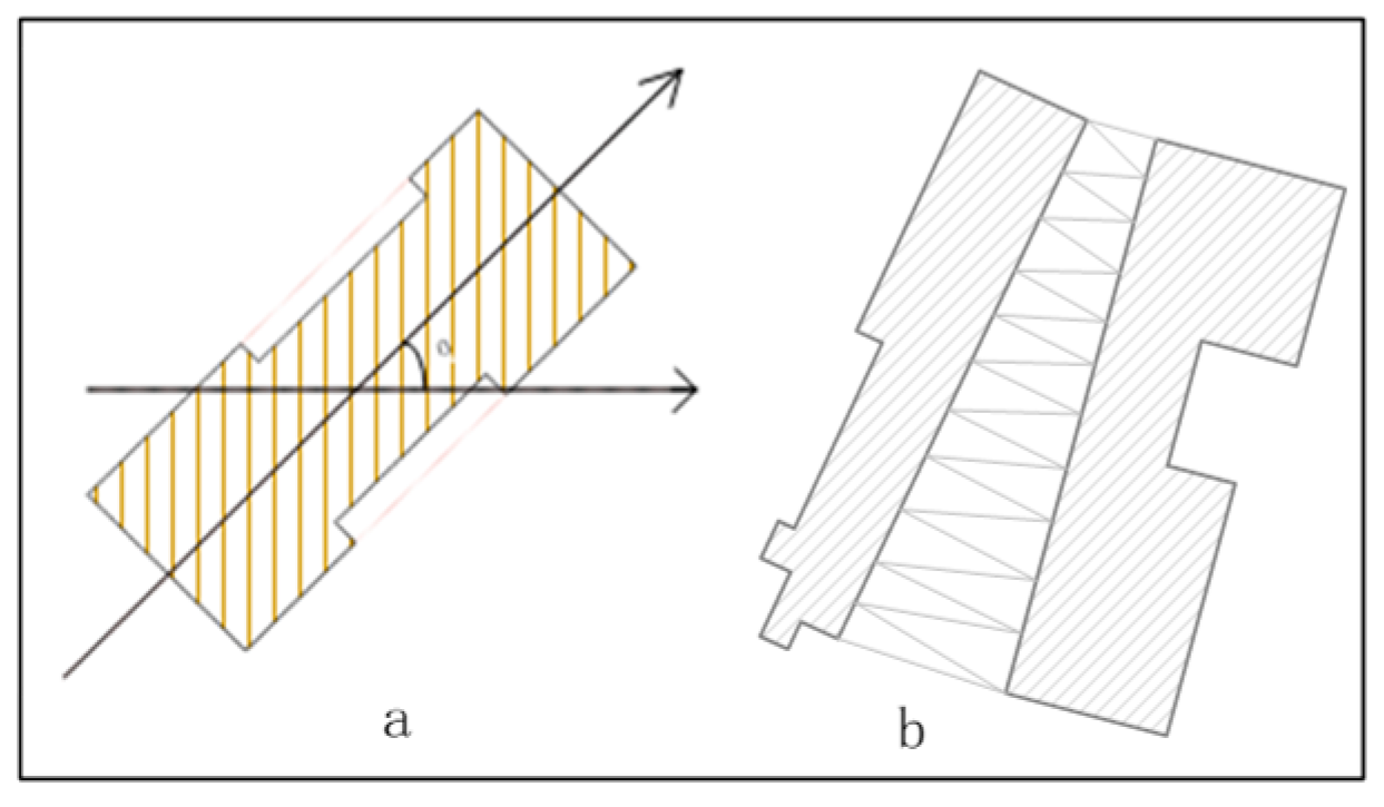
Considering polygon construction and relevant investigations that have been previously published [15], we fuzzified the following polygon information features to construct adjacency graph models (Table 1). A polygon’s shape was described by three indices: length–width ratio (LWR), solid degree (SD), and edge number (EN). A polygon’s direction was described by its orientation (O). A polygon size was described by calculating its area (A) and perimeter (P). Distance (D) and connectivity (C) were used to describe the neighborhood relationship of polygons.
Since the properties extracted from urban polygons have scale differences, fuzzifying them directly may obscure the effects of certain properties with small values. Therefore, different scales of the extracted properties were normalized using
x = x min max min ,
where x is original crisp of a certain property, x is the property of a certain index, and min and max are the minimal and maximum values of this particular property. This normalization approach was standardized for min-max, which is a linear transformation of the raw data whereby the resulting raw data is mapped between [0–1]. The standardized transformation process can unify dimension of index properties, which is beneficial for their fuzzification.

2.2. The EIFS-IBA Similarity Approach in Polygons

2.2.1. IBA Theory on Polygons

IBA contains all Boolean axioms and realized Boolean algebra in real-value ([0,1]-valued), which can depict objects with multiple properties. The origin framework of IBA is a generalized Boolean polynomial (GBP) [32], whose polynomials consist of Boolean algebra variables and operators standard +, standard -, and generalized product (GP). As GP operator is a subclass of t-norms; the four axioms (commutative, associative, monotone, and boundary condition and non-negativity) are also effective. Among various GP operators, min (GP: = min) is only suitable for depicting multi properties of objects [29]. Supposing primary variables Ω = { b 1 ,   b 1 b m }. Define two elements S ( a 1 ,   a 1 a m ) and T ( a 1 ,   a 1 a m ) as belonging to Boolean Algebra BA( Ω ). When GP is min, the IBA operation is performed based on the following formulae (GP: = min):
( S T ) = min   ( min ( S ) ,   min ( T ) ) ( S T ) = min ( S ) + min ( T ) min   ( min ( S ) ,   min ( T ) ) , ( ¬ S )   = 1 min ( S )
This formula denotes the IBA operation of two different objects; the operation can select the collective part of two objects with less information loss.
IBA is a strict mathematical operation which can be combined with IFS to express similarities between polygons. IFS originates from IF [22]. However, the generalization was first described in [23]. In Atanassov’s definition, an intuitionistic fuzzy set A in a universe E is
A = { ( x , μ A ( x ) , v A ( x ) | x     E ) } = < μ A , v A > ,
where functions μ A (x): E → [0, 1] and v A (x): E → [0, 1] denote the degree of membership and the degree of non-membership of the element x to the IFS A, respectively. As the sum of degrees of membership and non-membership is no more than 1, IFS may include another degree of uncertainty π A (x) of the membership of the element x ∈ E to A:
π A = 1 ( μ A + v A )
With the emergence of non-membership and uncertainty, IFS can provide a richer semantic description compared to fuzzy sets. However, since π A investigations are not as valid as membership and non-membership [29], we define the situation that μ A + v A = 1, and ignore the existence of π A .
Having acquired relevant theories on IFS, we can apply the specific IBA operation into IFS. Define two polygons O A { μ A , v A } and O B { μ B , v B }, and the logical operations of conjunction, disjunction, and negation within the IFS-IBA approach (GP: = min) should use the following formulae:
( O A O B ) = < min ( μ A ,   μ B ) ,   v A + v B min ( v A ,   v B ) > ( O A O B ) = < μ A + μ B min ( μ A ,   μ B ) ,   min ( v A ,   v B ) > ( ¬ O A ) = < v A , 1 v A >
In addition, the definition of IFS [28] IFS-IBA operation investigations revealed the rule on operating polygons:
( μ A v A ) = min ( μ A ,   v A ) = 0
When expressing similarities with a strict mathematical logic axiom, more detail of objects’ properties will be preserved. As a result, more meaningful spatial clustering results can be derived for more precise similarities.

2.2.2. EIFS-IBA Similarity Approach

The IBA theory, which has a strict mathematical logic axiom, performs well in measuring similarities/distances between non-spatial objects [29]. However, polygons are largely different from non-spatial objects, which contain extra proximity and spatial distances. Additionally, the roles of different spatial properties clearly vary in measuring similarities between polygons. To resolve this issue, we propose the Extend Intuitionistic Fuzzy Set-Interpolation Boolean Algebra similarity approach. The main advantage of the EIFS-IBA similarity approach over the original IFS-IBA is that it provides more complete, formal, and explicit sets. The formal description of EIFS-IBA can be represented as
EIFS IBA = { P o A ,   P o B ,   S ,   W ,   R ,   G } ,
where P o A refers to the properties of polygons, such as the properties in shape, direction, and size; P o B refers to the properties between adjacent polygons, such as proximity and spatial distance; S refers to the similarity in polygon pairs, such as polygons O A and O B ; W refers to the corresponding weight of each polygon property; R refers to the adjacent relation graph of contiguous polygons; and G refers to the final similarity graph model. In Equation (7), the sets of P o A and S were elements of the original IFS-IBA approach. Compared with our proposed approach, conventional IFS-IBA did not provide sufficient information about polygon properties and configurations. We explain sets P o A , P o B , S, and W in the following statement; sets R and G are arranged in Section 2.3.
To depict spatial properties of polygon P o A (such as orientation and area) in the EIFS-IBA similarity approach, the extracted spatial properties were first normalized into a [0,1]-interval crisps μ o F via data preprocessing. Then, we transformed the obtained crisps μ o F into membership μ o A and non-membership v o A . Among various transformation approaches [33,34], the maximum intuitionistic fuzzy entropy principle [34] with λ ≥ 0 proved to be suitable for depicting objects [29]:
μ o A = 1 ( 1 μ o F ) λ v o A = ( 1 μ o F ) λ ( 1 + λ )
The value λ plays an important role in the transformation process; an expert in the case of IF clustering [35] suggests that λ = 0.95. Polygon P o A properties were derived in the following manner:
P o A = ( μ o A ,   v o A )
Distinct from the spatial properties of polygon P o A , the properties between adjacent polygons P o B were acquired differently [17]. The properties between adjacent polygons P o B were derived using
P o B = ( D o AB ,   C o AB ) ,
where D o AB and C o AB are the distance and connectivity between two polygons, respectively. In our EIFS-IBA approach, s dis and s con are equal to D o AB and C o AB , respectively, and were derived from the Delaunay triangle and skeletons [17].
For polygon objects O A { μ A , v A } and O B { μ B , v B }, the similarity measurement (only containing polygon properties) satisfies the IFS-IBA equivalence relation. The well-known tautology [29] is still suitable for polygons:
A < = > B = ( A ^ B ) ( ˺ A ^ ˺ B )
As a result, the operation can be derived in the following manner [29] (GP:   = min):
( O A < = > O B ) = ( O A ^ O B ) ( ˺ O A ^ ˺ O B ) = { ( < μ A , V A > ^ < μ B , V B > ) ( ˺ < μ A , V A > ^ ˺ < μ B , V B > ) }   = < min ( μ A , μ B ) + min ( V A , V B ) ,   V A + V B 2 min ( V A , V B ) > ,
When measuring similarities between polygons, only the membership of IFS is vital. The similarities of non-spatial properties can be calculated using
S I ( O A ,   O B ) = { 1 , O A = O B min ( μ A , μ B )   +   min ( V A , V B ) ,   otherwise ,
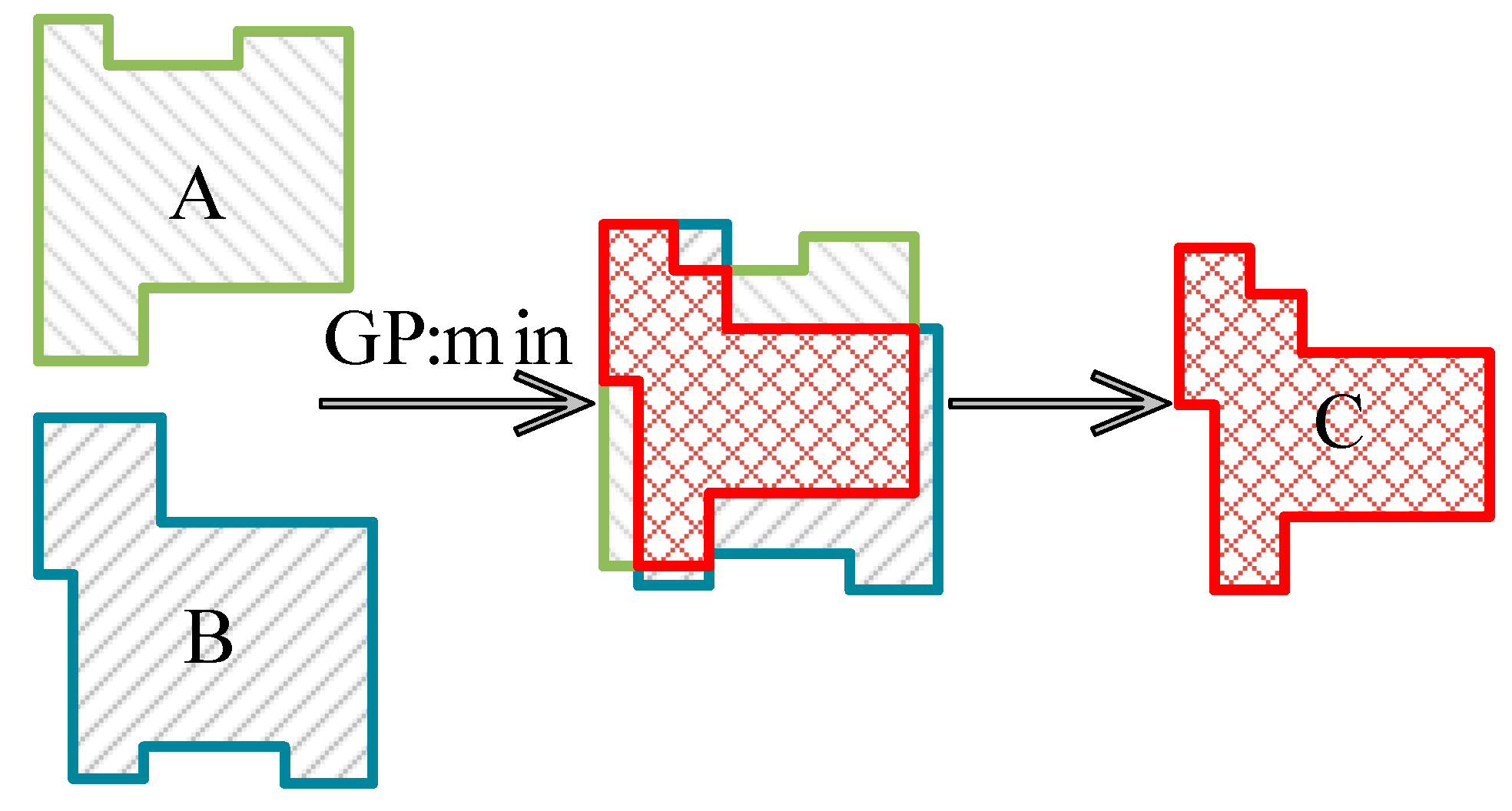
where S I is polygon similarities; for polygon objects O A and O B , the similarities can be denoted as 1 when the properties of the two are coincident. Otherwise, the similarities can be measured using the IFS-IBA operation. The similarity S I only contains polygon properties for the IFS theory, which cannot express the properties between polygons (such as spatial distance and proximity). Figure 3 interprets the IFS-IBA similarity theory. For object O A and O B , the similarity obtained using the IFS-IBA similarity approach is C (C is the properties that are part of A and B).
Spatial properties of polygons cannot provide sufficient information to depict similarities between them. Hence, other spatial properties, like distance and connectivity, are indispensable [36]. However, both distance and connectivity represent the relation between polygons, which cannot be depicted by the IFS-IBA approach directly. The S in our proposed EIFS-IBA approach resolves the issue. The formula is
S ( O A ,   O B ) = w i   ×   S I ( O A , O B ) + w 2   ×   s dis + w 3   ×   s con ,
where w i refers to the total weight of polygon properties in shape, orientation, and size, and S I ( O A , O B ) refers to the similarity of each property in shape, size, and orientation; and w 2 and w 3 refer to weights for distance and connectivity properties, respectively. The total weight of w i ,   w 2 , and w 3 is 1. When w i = 1, the S in IFS-IBA was consistent with S in the EIFS-IBA approach.
Different properties have different roles in polygons’ clustering. It is therefore crucial to provide a reasonable weight for each polygon property. In this paper, we used the Relief-F algorithm [30] to automatically optimize weights and reduce time consumption. W in the EIFS-IBA approach can be denoted in following manner:
W = ( w i ,   w 2 ,   w 3 )
The weight of each property can be trained with sample data. In general, the W in different datasets was slightly different.

2.3. The Graph Model and Partition of Polygons

Graph theory is a widely used method for representing the relationship between a set of polygons. In general, a simple graph G consists of a finite, non-empty set of nodes N (G) and edges E (G). Meanwhile, each edge E ij ( N i ,   N j ) connects nodes N i and N j in graph G.
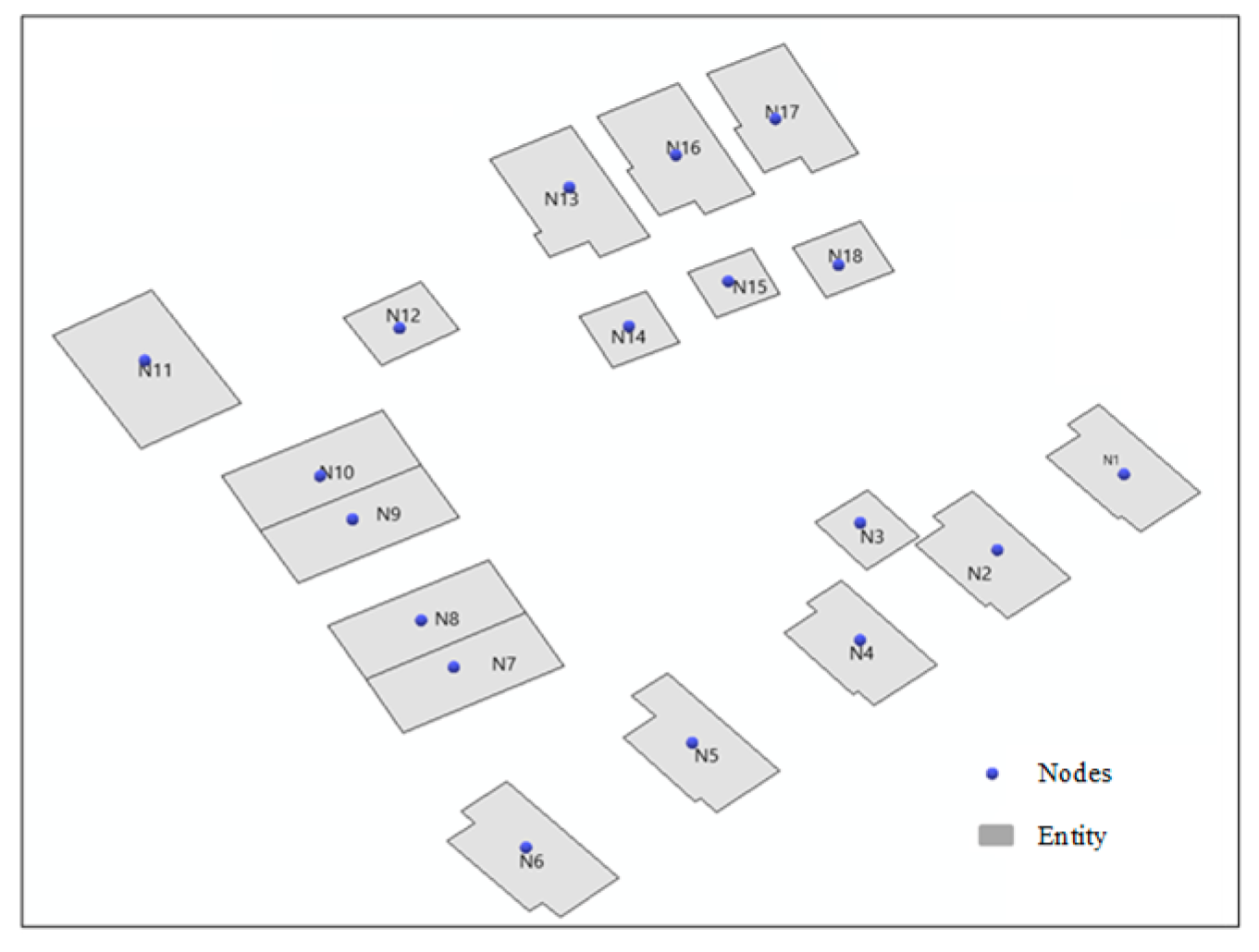
In the polygon’s adjacent graph model, each member of set N (G) in graph G corresponds to a unique urban object, and an edge E ij ( N i , N j ) between nodes N i and N j indicates that a relation exists between the corresponding polygons. Constructing the adjacency graph model between polygons began with polygons being coarsened into nodes (N). In this process, the centroid of polygons can be selected as coarsened nodes (N). Then, we constructed the Delaunay triangulation of the nodes to generate the adjacency relationship graph that contains the connection relationship between polygons. Finally, we calculated the value of edge (E) in the adjacency relationship graph and establish a competed adjacency graph (G). Calculating the value of each edge E ij ( N i , N j ), which is the similarity between adjacent polygons, is significant for constructing the adjacency graph model. The adjacency relationship graph model (AGM) that corresponds to R in EIFS-IBA can be achieved using the matrix
AGM = ( a 11 a 1 j a i 1 a ij ) ,
where a ij refers to the similarity between the two polygons (or polygon pair). If the polygons are not adjacent, we used 0 to denote the similarity between them. The AGM was used to identify whether two polygons were adjacent. As the polygon pairs were obtained from the Delaunay triangulation [37] of the nodes, the storage efficiency of the AGM matrix model was low. To resolve the dilemma, we established an extended adjacency relationship graph model (EAGM) corresponding to G in EIFS-IBA, which only contained the similarity of adjacent polygons, i.e.,
EAGM = ( w ij ) ,
where w ij refers to the similarity between the two polygons, corresponding to S in our EIFS-IBA approach. Figure 4 depicts the polygon adjacency graph model construction. For instance, w 12 (a1, a2) is the similarity between polygon a1 and a2; w 13 (a1, a3) will not arise in the EAGM, for a1 and a3 are not adjacent.
The partition process is the final step of clustering. As the multi-level graph partitioning approach performed well in the multi-property polygon clustering analysis, we partitioned the acquired graph model with similarities between polygons using the multi-level graph partitioning approach [17].

2.4. Evaluation of Clustering Quality

As clustering is an unsupervised process, clustering quality evaluation is of great importance. There are many clustering evaluation criteria; the silhouette coefficient and information entropy are superior in many methodologies [17]. In this paper, we chose the silhouette coefficients of the clustering results to evaluate their merits, and further used geometric features to validate the results.

2.4.1. Silhouette Coefficient

The silhouette coefficient [38] is a method used for evaluating clustering effectiveness using the pairwise difference between- and within-cluster distance. For a polygon v i in a cluster, its silhouette s(i) is defined as
s ( i ) = b ( i ) a ( i ) max { a ( i ) , b ( i ) } ,
where s(i) ranges from −1 to 1, a(i) measures the compactness of the cluster containing v i , and b(i) captures the degree to which v i is separated from the other clusters. A larger s(i) implies that the cluster containing v i is compact and v i is far away from the other clusters. However, when s(i) is negative (i.e., b(i) < a(i)), v i is closer to the polygons in other clusters.

2.4.2. The Information Content of the Geometric Features

The information content of geometric features (ICGF) of polygons is generated using the complex diversity of polygon geometries. The geometric shape of complex surface elements can be decomposed into the convex tree node polygons and their mutual relationships. The ICGF ( A i ) of individual polygon element A i [39] is
I ( A i ) = j = 1 m i w ij log 2 ( 1 + ne ij ) ( 2 C ij ) ( l ij + 1 ) ( d ij + 1 ) ,
where m i refers to the number of convex hulls generated by A i decomposition; ne ij refers to the ratio of the number of polygon edges to the average number of edges in the pocket nodes of the convex hull tree; C ij refers to the solidity of the pocket polygon of the convex hull tree node; l ij refers to the ratio of the number of layers in the convex hull tree node and the average number of layers; d ij refers to the ratio of out-degree and average out-degree of the convex hull tree node; and w ij refers to the area weight, which is the ratio of the area of the convex hull to the area of the largest convex hull.
The ICGF is related to the geometric shape of the polygons in each polygon. The geometric features of each polygon are independent of each other. We calculated the weight of each polygon according to the area and then the weight and sum of geometric features for all polygon features, finally acquiring the ICGF of the polygon I g , which is
I g = i = 1 m w i I ( A i ) ,
w i = s i / s ¯ ,
where s ¯ refers to the average area factor of polygons; m is the total number of polygons; and w i refers to area weight, which is the area ratio of the features to the mean value. The geometric feature information performance of the clustering results is described by calculating the difference in ICGF between adjacent clusters. Having known the ICGF of each cluster from the different similarity approaches, we constructed a graph model containing adjacent clusters and calculated the ICGF difference between them.

3. Results

3.1. Dataset

In this study, we applied the proposed method to Staten Island. Staten Island, which is one of the five boroughs of New York City, is located in the southernmost part of New York City. The geometric features and spatial distribution of polygons in Staten Island are complex and diverse, and it represents a more general polygon distribution pattern. Hence, we chose polygons in Staten Island to study their clustering, given that the complicated polygon distribution in Staten Island can fully demonstrate the applicability of the EIFS-IBA similarity approach. To further verify the applicability and reliability of the presented approach, we analyzed the regions outlined by red boxes in Figure 5. Experimental region b was first partitioned according to human cognition to train the weight of each index using the Relief-F algorithm. Then, we conducted the whole process using the proposed approach in experimental region a. Finally, comparative analysis using different similarity approaches was performed in experimental region c. The footprint in vector format of New York City was released by the NYC Department of Information Technology and Telecommunications (DoITT, http://www1.nyc.gov/site/doitt/index.page, accessed July 2017).

3.2. Experiment Setting and Clustering Results

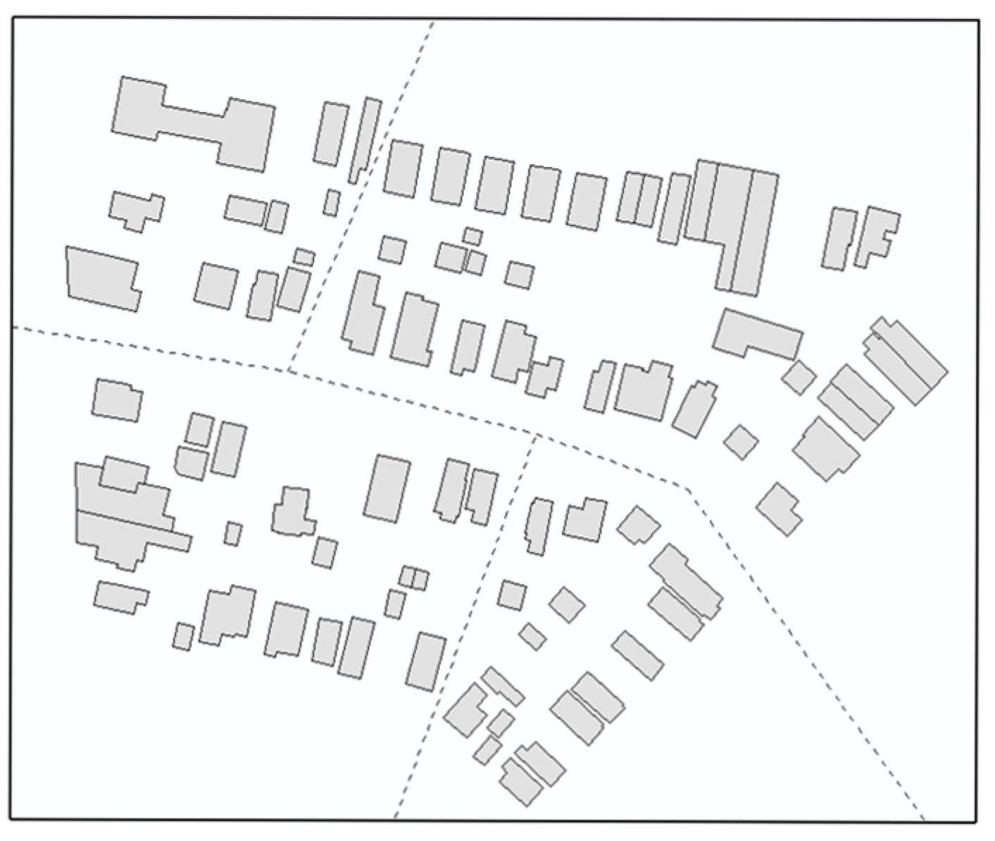
Selecting similarity properties and their corresponding weights affects the calculated similarity between polygons, which has a further significant influence on the cluster result. This study aimed to cluster polygons in a manner consist with human cognition, so we trained the sample (Figure 6) to acquire the corresponding weight of each property using the Relief-F algorithm shown in Table 2.
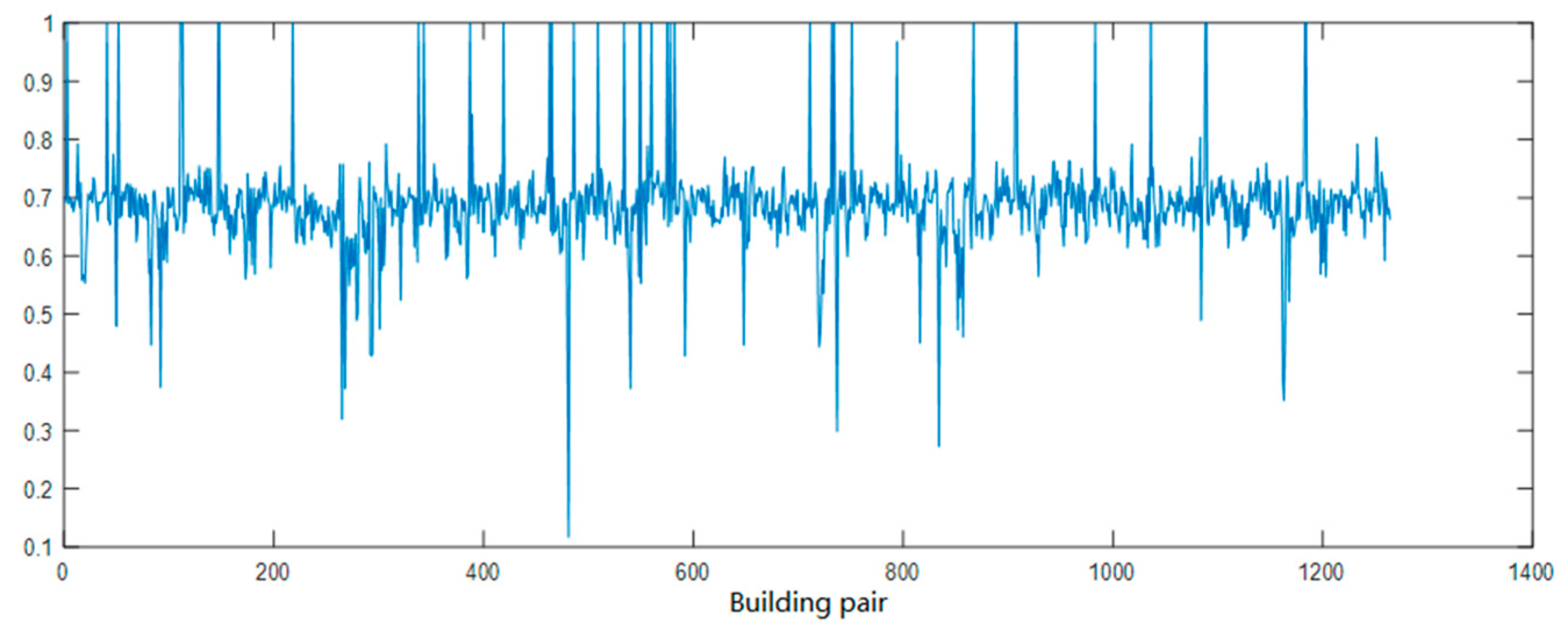
Table 3 is the adjacency graph model of experimental region a. The maximum similarity (edge weights) between the polygons is 1, indicating that the two polygons are linked together. The minimum value is 0.1167 (given the large amount of data, this value is not shown in Table 4); and the similarity between most polygon pairs is ~0.70 (Figure 7). The similarity between these polygon pairs allowed us to partition in the next step. After constructing the adjacency graph model containing polygon neighbor information, we used the multi-level graph partitioning approach to complete the clustering.
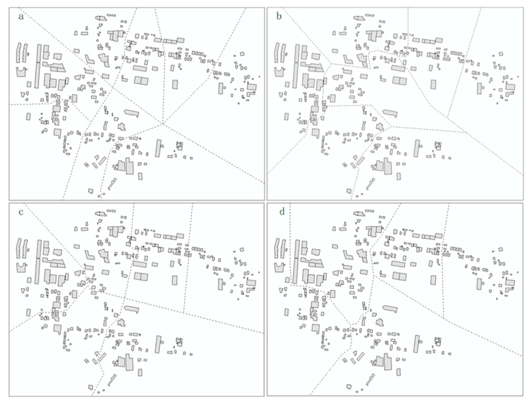
After completing the similarity property and weights analysis, we set the similarity thresholds of the multi-level graph partitioning approach to 75%, 70%, 65%, and 60% according to the distribution of similarity in experimental region a. Figure 8 shows the partitioned results of experimental region a. However, due to the complexity of polygon distribution in the experimental region, it was difficult to distinguish the effect with simple human vision. Hence, further assessment and analysis are necessary.
By analyzing the clustering results of experimental region a under different thresholds (Figure 8), we found that the number of clusters gradually decreased with the gradual reduction in partition threshold (from 75% to 60%) as the number of polygons per cluster increased and the total number of clusters naturally decreased. Secondly, the silhouette coefficients (Table 4) with different thresholds varied greatly. When setting the similarity threshold to 70%, the silhouette coefficient values reached the maximum. When the threshold gradient was 5%, setting the similarity threshold to about 70% generated better results. The number of polygon pairs above or below 0.7 was relatively rare; the threshold outside this range (~70%) was not conducive to better results. If the threshold is too small, the cluster result is not fully partitioned. Otherwise, the clusters are over partitioned.

3.3. Comparison and Analysis of Different Similarity Approaches

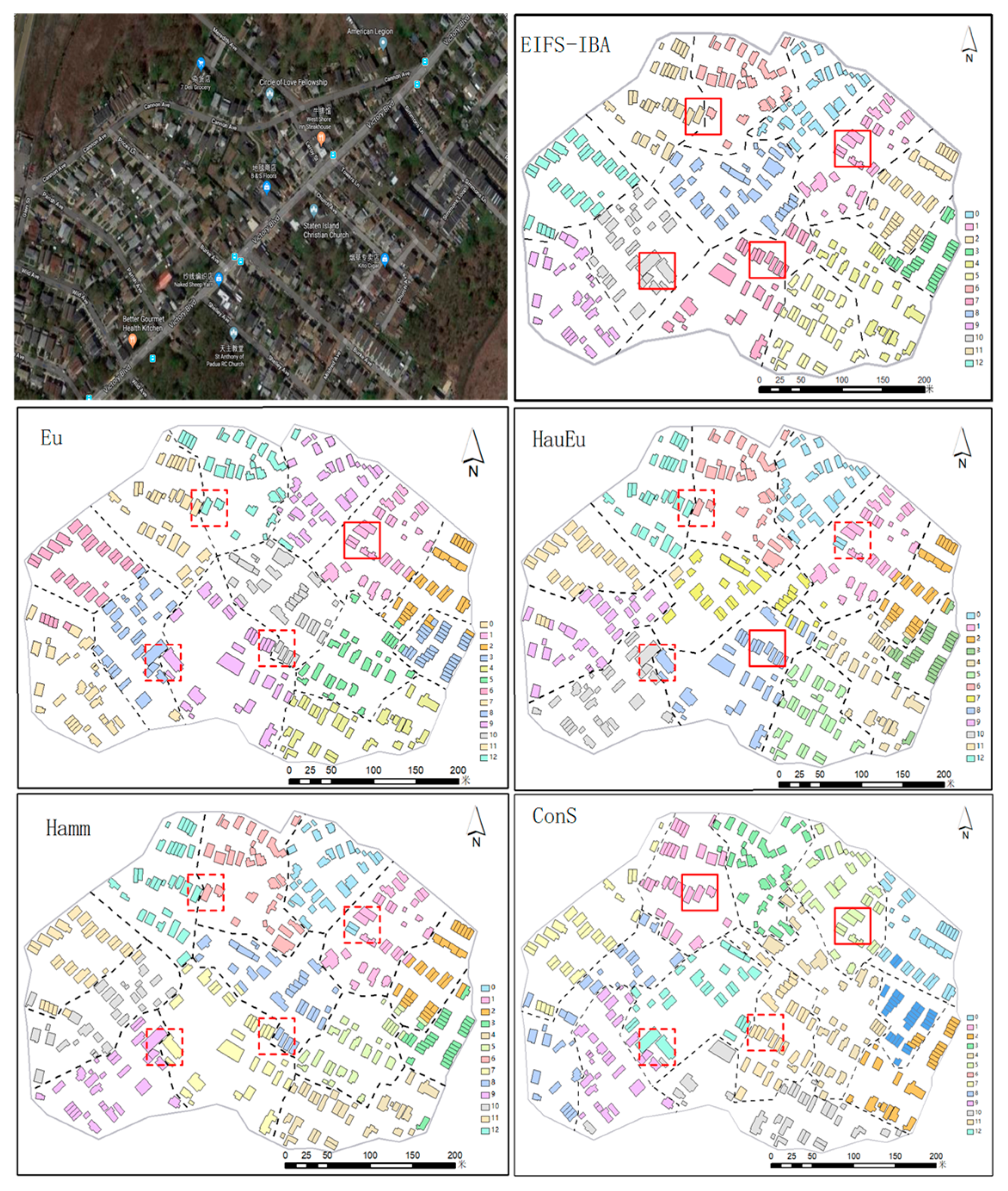
We then performed further analysis and comparison of the clustering results in experimental region c which were operated by various similarity approaches (including EIFS-IBA, normalized Euclidean (Eu), Hausdorf Euclidean (HauEu), normalized Hamming (Hamm), and conventional similarity (ConS); see Table 5). When setting the similarity threshold to 70% and applying each index weight as shown in Table 2, the clustering partitions were completed by different similarity approaches. Clusters (Figure 9) of the four fuzzy similarity approaches were similar in polygon volume and spatial characteristics within clusters. There were some clusters of abnormal shape in the ConS approach. For example, the region of cluster number 8 was approximately character ‘C’, and the boundary near cluster 9 was not clear. The overall visual cognition cannot rigorously evaluate the quality of the clustering result, so it still essential to use the silhouette coefficient to carry on further evaluation.
Table 6 shows the silhouette coefficients of experimental region c using five different similarity approaches under the same parameter settings. The EIFS-IBA similarity approach had the best performance, while the ConS approach performed the worst. By comparing the silhouette coefficients between the two, the EIFS-IBA had up to 25% improvement. In addition, the other three fuzzy similarity approaches all had different degrees of improvement. However, because the mechanism of similarity expressions is different, the improvement effect is not as significant as that of EIFS-IBA.
We further assessed the four areas marked by red rectangular boxes in the experimental region in Figure 9 (dotted lines indicate that the area did not meet visual cognition and the solid line is consistent with cognition) and analyzed the effect of the EIFS-IBA similarity approach from a local perspective. The four solid red rectangles indicated that the EIFS-IBA similarity approach partition did not significantly violate human visual perception. For example, the uppermost region of the figure partitioned two neighboring polygons—whose shape and area were significantly different in different clusters—instead of being partitioned into the same cluster only based on distance. As for the other fuzzy similarity approaches, only one area of Eu and HauEu was consistent with cognition, and Hamm was totally against human cognition. Although ConS had two cognitive areas, the overall division results differed significantly from cognitive criteria. As a whole, fuzzy sets had significant advantages with regards to similarity expression. Furthermore, an appropriate express manner is particularly important in the application of polygon cluster analysis. The adopted EIFS-IBA similarity approach has obvious advantages in polygon clustering analysis.

3.4. Verification by the Differences Between ICGF

The geometric features between polygons in the same cluster are of relevance, and therefore, the clustering results can be evaluated by comparing the differences between ICGF in adjacent clusters. The ICGF of clusters according to different similarity approaches are shown in Table 7.
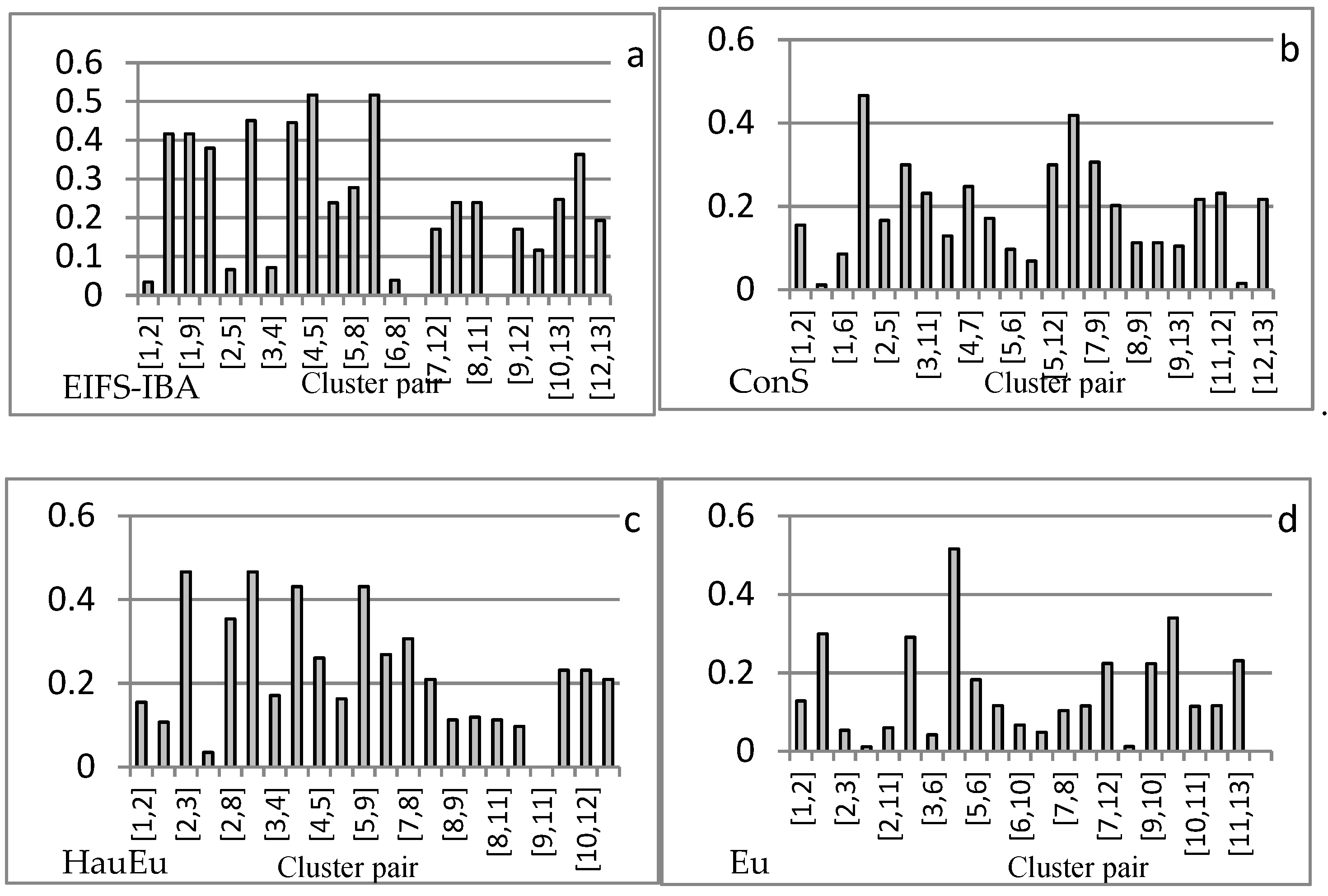
Table 7 represents statistical information on the ICGF of clusters in Figure 9; the numerical values in each row are the ICGF for corresponding clusters (i.e., the data in the first column corresponds to clusters in the clustering result obtained by the EIFS-IBA similarity approach in Figure 9). According to Section 2.4.2, ICGF differences can be evaluated based on the effect in the perspective cluster pair. After acquiring the adjacent relation of clusters in Figure 9, we summarized ICGF differences and excellence rates in Figure 10.
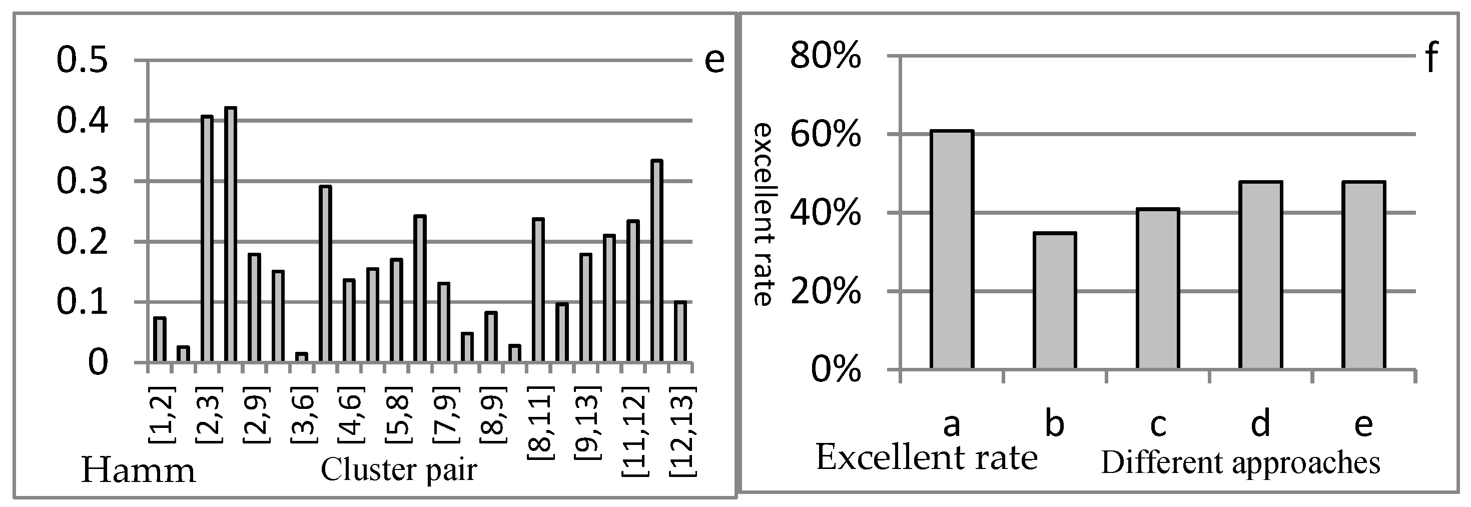
Figure 10 shows the range for which ICGF differences was [0, 0.51] and where a, b, c, d, e, and f corresponded to the EIFS-IBA, ConS, HauEu, Eu, and Hamm similarity approaches and excellence rates, respectively; and where the horizontal axis in a, b, c, d, and e represented an adjacent cluster pair. For example, [1, 2] (which is cluster 1 and cluster 2) corresponded to the 0 and 1 regions in Figure 9; the vertical axis is the difference in the ICGF. By combining the EIFS-IBA clustering results in Figure 9, the adjacent cluster differences can be divided into three ranges: [0, 0.1], [0.1, 0.3], and [0.3, 0.51]. When the difference range is [0, 0.1] and the cluster pair [1, 2] is taken as an example, we found a clear interval between the corresponding 0 and 1 regions, indicating that the location was close to the dominant relationship and the results were reasonable. When the difference range was [0.1, 0.3] and the cluster pair [9, 12] was used as an example, we found that the corresponding positional relationship between the 8 and 11 regions was not obvious. Polygons’ ICGF values in their respective regions were quite different, and the ICGF of the two regions were averaged. As a result, ICGF differences in the two regions were not significant, showing that the division results of the two regions were mediocre. When the difference range was [0.3, 0.51] and the cluster pair [4, 5] was taken as an example, we found that the corresponding positional relationship between regions 3 and 4 regions was not obvious, but the ICGF difference between the two regions was relatively large, indicating that the geometric features were dominant, thus giving reasonable results. Hence, it can be concluded that the ranges [0, 0.1] and [0.3, 0.51] belong to the favorable division. These two ranges correspond to results of the significant partition of the neighborhood relationship or geometric features, respectively. In the range [0.1, 0.3] there may be more negative partitions. The clusters contained more incorrectly partitioned boundary polygons in which the difference in the ICGF was large. The average ICGF was closed to an intermediate value, which ultimately led to differences in ICGF information between clusters in this range. Thus, the distribution range of the statistical cluster differences can reflect the dependence of polygons in the same clusters. Furthermore, the excellent rate of partition results can reflect the performance of clustering results based on different approaches.
The first five graphs in Figure 10 show cluster pairs’ (between adjacent clusters) ICGF differences, and the last graph is the excellence rate of the different similarity approaches. It can be found that the performance of EIFS-IBA was predominantly better than the other approaches, followed by the other three fuzzy set approaches; the ConS approach performed the worst. The performance was also similar to the previous silhouette coefficients, which fully showed the strong information expression ability of the fuzzy sets, and the appropriate similarity approach was more conducive to polygon clustering, which was in accordance with the cognitive criteria.

4. Discussion

It is essential to describe polygon property information accurately as a condition of differentiation during polygon clustering. As the conventional similarity approach simply handles the similarity properties, it is difficult to include detailed feature information representing polygons. To resolve the issue, we have proposed the EIFS-IBA similarity approach, which is very flexible and has some outstanding advantages over ConS methods. First, we dealt with the properties of a single polygon, which is consistent with the way that humans or computers come into contact with city scenes. In the fuzzy similarity, the geometric spatial information of the direction, shape, and size of the polygon was added to improve the information richness. This information can better express the polygon attributes and establish a more accurate attribute relationship for clustering so as to obtain better clustering results. Secondly, the EIFS-IBA similarity approach has a strict mathematics foundation which is derived from the argument of equivalent substitution and is logically rigorous. More importantly, the EIFS-IBA similarity approach has strong expressive ability and can accurately describe the relationships between polygon entities, which is more advantageous than conventional ways that calculate it from ratios or differences.
The fuzzy set theory is relatively mature and performs well in clustering, partitioning, and pattern recognition. However, the application of clustering in geographic information systems is relatively rare. In this paper, we have proposed the EIFS-IBA similarity approach that has a strong capability of information expression and integration to measure polygon similarities. The experiments showed that the similarities acquired by the EIFS-IBA similarity approach have a good effect on clustering. However, the effectiveness of the EIFS-IBA similarity clustering experiment is still affected by the following factors: first, in fuzzy set application, we only adopt the currently applied mature degree of membership and non-membership, and do not apply the third uncertainty index of the fuzzy concentration, which will affect the powerful information expression of the EIFS-IBA approach to a certain extent; second, although the spatial attribute features used in this paper are rich, there may still exist other potentially more effective attribute indices, such as POI, etc. Even multiple attributes may interact with each other to further affect clustering.

5. Conclusions

Polygon clustering is one of the most important tasks of data mining. Most of the current similarity calculation approaches for clustering mining experiments remain at a certain level, and do not further explore the potential of similarity approaches. On the one hand, the mechanisms of current similarity approaches are quite primitive and the acquired similarity cannot show details of the similar part. On the other hand, current mathematical sciences have reached a higher level in the study of similarity approaches, which has explored the advanced similarity that can express the additional detail of similar parts. However, there are fewer theories applied to geographic information systems. The major contribution of this work is the designed EIFS-IBA similarity approach, which can measure similarities between polygons.
This paper overcomes the drawbacks of the conventional IFS-IBA approach that cannot measure the spatial relation between spatial objects. In this paper, we first extracted spatial properties (such as area, shape, and orientation, etc.). Then we applied IFS-IBA to measure the properties of spatial objects and measure the additional similarities between spatial objects (length and connectivity). Finally, we conducted spatial clustering with the weight similarity between spatial objects. Both the visual result and evaluation criteria demonstrate that the EIFS-IBA similarity approach can partition complex polygons in accordance with visual recognition results. In addition, our proposed EIFS-IBA similarity approach is expressive and therefore can be applied to many geographical information analyses which utilize similarity. Furthermore, we will also explore the impact of the uncertainty in the EIFS-IBA similarity approach, and of membership and non-membership on the ability to express similarities in geographic information. In future work, we aim to explore cluster analysis tools that are more conducive to mining hidden information in spatial data.
Author Contributions

Zhanlong Chen conceived and designed the experiments and performed the modeling; Xiaochuan Ma analyzed the data and reviewed and edited the draft. All authors discussed the basic structure of the manuscript and read and approved the manuscript.

Funding

This work was supported by the National Natural Science Foundation of China (No. 41871305), the National Key R&D Program of China (2017YFC0602204), the Fundamental Research Funds for the Central Universities, China University of Geosciences (Wuhan) (No. CUG160226), and the Open Research Fund of the Teaching Laboratory of China University of Geosciences (No. skj2014168).

Acknowledgments

The authors thank the editors for their patience and opinions.

Conflicts of Interest

The authors declare no conflict of interest.

References

  1. Wu, X.; Zhu, X.; Wu, G.Q.; Ding, W. Data mining with big data. IEEE Trans. Knowl. Data Eng. 2013, 26, 97–107. [Google Scholar]
  2. Li, Z.; Liu, Q.; Tang, J. Towards a Scale-driven Theory for Spatial Clustering. Acta Geod. Et Cartogr. Sin. 2017, 46, 1534–1548. [Google Scholar]
  3. Wang, X.; Rostoker, C.; Hamilton, H.J. A density-based spatial clustering for physical constraints. J. Intell. Inf. Syst. 2012, 38, 269–297. [Google Scholar] [CrossRef]
  4. Kulldorff, M.; Nagarwalla, N. Spatial disease clusters: Detection and inference. Stat. Med. 1995, 14, 799–810. [Google Scholar] [CrossRef] [PubMed]
  5. Fovell, R.G.; Fovell, M.Y.C. Climate Zones of the Conterminous United States Defined Using Cluster Analysis. J. Clim. 1993, 6, 2103–2135. [Google Scholar] [CrossRef] [Green Version]
  6. Zaliapin, I.; Ben-Zion, Y. Earthquake clusters in southern California I: Identification and stability. J. Geophys. Res. Solid Earth 2013, 118, 2847–2864. [Google Scholar] [CrossRef] [Green Version]
  7. Drǎguţ, L.; Tiede, D.; Levick, S.R. ESP: A tool to estimate scale parameter for multiresolution image segmentation of remotely sensed data. Int. J. Geogr. Inf. Sci. 2010, 24, 859–871. [Google Scholar] [CrossRef]
  8. Yan, H.; Weibel, R.; Yang, B. A multi-parameter approach to automated building grouping and generalization. Geoinformatica 2008, 12, 73–89. [Google Scholar] [CrossRef]
  9. Joshi, D. Polygonal Spatial Clustering. Unpublished Ph.D. Thesis, Department of Computer Science and Engineering, University of Nebraska at Lincoln, Lincoln, NE, USA, 2011; pp. 334–346. [Google Scholar]
  10. Macqueen, J. Some Methods for Classification and Analysis of MultiVariate Observations. In Proceedings of the Fifth Berkeley Symposium on Mathematical Statistics and Probability; University of California Press: Berkeley, CA, USA, 1965; Volume 23, pp. 281–297. [Google Scholar]
  11. Kohonen, T. Self-organized formation of topologically correct feature maps. Biol. Cybern. 1982, 43, 59–69. [Google Scholar] [CrossRef]
  12. Gennari, J.H.; Langley, P.; Fisher, D. Models of incremental concept formation. Artif. Intell. 1989, 40, 11–61. [Google Scholar] [CrossRef]
  13. Zhang, T. An Efficient Data Clustering Method for Very Large Databases. ACM Sigmod Rec. 1996, 25, 103–114. [Google Scholar] [CrossRef]
  14. Ester, M.; Kriegel, H.-P.; Sander, J.; Xu, X. A density-based algorithm for discovering clusters in large spatial databases with noise. Proc. Kdd 1996, 18, 226–231. [Google Scholar]
  15. Cetinkaya, S.; Basaraner, M.; Burghardt, D. Proximity-based grouping of buildings in urban blocks: A comparison of four algorithms. Geocarto Int. 2015, 30, 618–632. [Google Scholar] [CrossRef]
  16. Ng, R.T.; Han, J. Efficient and Effective Clustering Methods for Spatial Data Mining; University of British Columbia: Vancouver, BC, Canada, 1994; pp. 144–155. [Google Scholar]
  17. Wang, W.; Du, S.; Guo, Z.; Luo, L. Polygonal Clustering Analysis Using Multilevel Graph-Partition. Trans. GIS 2015, 19, 716–736. [Google Scholar] [CrossRef]
  18. Sander, J.; Ester, M.; Kriegel, H.-P.; Xu, X. Density-based clustering in spatial databases: The algorithm gdbscan and its applications. Data Min. Knowl. Discov. 1998, 2, 169–194. [Google Scholar] [CrossRef]
  19. Guo, D.; Wang, H. Automatic region building for spatial analysis. Trans. GIS 2011, 15, 29–45. [Google Scholar] [CrossRef]
  20. Zhang, X.; Ai, T.; Stoter, J.; Kraak, M.-J.; Molenaar, M. Building pattern recognition in topographic data: Examples on collinear and curvilinear alignments. Geoinformatica 2013, 17, 1–33. [Google Scholar] [CrossRef]
  21. Zhao, H.; Xu, Z.; Liu, S.; Wang, Z. Intuitionistic fuzzy MST clustering algorithms. Comput. Ind. Eng. 2012, 62, 1130–1140. [Google Scholar] [CrossRef]
  22. Zadeh, L.A. Fuzzy sets. Inf. Control 1965, 8, 338–353. [Google Scholar] [CrossRef] [Green Version]
  23. Atanassov, K.T. Intuitionistic fuzzy sets. Fuzzy Sets Syst. 1986, 20, 87–96. [Google Scholar] [CrossRef]
  24. Hwang, C.-M.; Yang, M.-S.; Hung, W.-L.; Lee, M.-G. A similarity measure of intuitionistic fuzzy sets based on the Sugeno integral with its application to pattern recognition. Inf. Sci. 2012, 189, 93–109. [Google Scholar] [CrossRef]
  25. Wang, Z.; Xu, Z.; Liu, S.; Yao, Z. Direct clustering analysis based on intuitionistic fuzzy implication. Appl. Soft Comput. J. 2014, 23, 1–8. [Google Scholar] [CrossRef]
  26. Nguyen, H. A novel similarity/dissimilarity measure for intuitionistic fuzzy sets and its application in pattern recognition. Expert Syst. Appl. 2016, 45, 97–107. [Google Scholar] [CrossRef]
  27. Szmidt, E.; Kacprzyk, J. Distances between intuitionistic fuzzy sets. Fuzzy Sets Syst. 2000, 114, 505–518. [Google Scholar] [CrossRef]
  28. Milosevic, P.; Poledica, A.; Rakicevic, A.; Petrovic, B.; Radojevic, D. Introducing Interpolative Boolean algebra into Intuitionistic fuzzy sets. Mathw. Soft Comput. 2015, 22, 30–31. [Google Scholar]
  29. Milošević, P.; Petrović, B.; Jeremić, V. IFS-IBA similarity measure in machine learning algorithms. Expert Syst. Appl. 2017, 89, 296–305. [Google Scholar] [CrossRef]
  30. Kononenko, I. Estimating attributes: Analysis and extensions of RELIEF. In European Conference on Machine Learning; Springer: Berlin/Heidelberg, Germany, 2009; Volume 13, pp. 171–182. [Google Scholar]
  31. Yu, B.; Liu, H.; Wu, J.; Hu, Y.; Zhang, L. Automated derivation of urban building density information using airborne LiDAR data and object-based method. Landsc. Urban Plan. 2010, 98, 210–219. [Google Scholar] [CrossRef]
  32. Radojević, D. (0, 1)-valued logic: A natural generalization of Boolean logic. Yugosl. J. Oper. Res. 2000, 10, 185–216. [Google Scholar]
  33. Bustince, H.; Kacprzyk, J.; Mohedano, V. Intuitionistic fuzzy generators Application to intuitionistic fuzzy complementation. Fuzzy Sets Syst. 2000, 114, 485–504. [Google Scholar] [CrossRef]
  34. Vlachos, I.K.; Sergiadis, G.D. The role of entropy in intuitionistic fuzzy contrast enhancement. In International Fuzzy Systems Association World Congress; Springer: Berlin/Heidelberg, Germany, 2007; Volume 45, pp. 104–113. [Google Scholar]
  35. Visalakshi, N.K.; Parvathavarthini, S.; Thangavel, K. An intuitionistic fuzzy approach to fuzzy clustering of numerical dataset. In Computational Intelligence, Cyber Security and Computational Models; Springer: New Delhi, India, 2014; Volume 34, pp. 79–87. [Google Scholar]
  36. Du, S.; Luo, L.; Cao, K.; Shu, M. Extracting building patterns with multilevel graph partition and building grouping. ISPRS J. Photogramm. Remote Sens. 2016, 122, 81–96. [Google Scholar] [CrossRef]
  37. Deng, M.; Liu, Q.; Cheng, T.; Shi, Y. An adaptive spatial clustering algorithm based on Delaunay triangulation. Comput. Environ. Urban Syst. 2011, 35, 320–332. [Google Scholar] [CrossRef]
  38. Kaufman, L.; Rousseeuw, P.J. Finding Groups in Data: An Introduction to Cluster Analysis; John Wiley & Sons: Hoboken, NJ, USA, 1990; Volume 8, pp. 329–344. [Google Scholar]
  39. Liu, H.; Deng, M.; Fan, Z.; Lu, Q. A Characteristics-based Approach to Measuring Spatial Information Content of the Settlements in a Map. Acta Geod. Et Cartogr. Sin. 2014, 10, 1–18. [Google Scholar]
Figure 1. Numbering spatial polygons.
Ijgi 08 00098 g001
Figure 2. Explanation of the relative concept. (a) Smallest bounding rectangle and orientation. (b) Skeletons between adjacent polygons.
Ijgi 08 00098 g002
Figure 3. Graphical interpretation of the Intuitionistic Fuzzy Set-Interpolation Boolean Algebra (IFS-IBA) operation on polygons. Legend: GP, generalized product.
Ijgi 08 00098 g003
Figure 4. Adjacency relationship graph. (a) The polygon; (b) the constructed adjacency relationship graph; and (c) the corresponding extended adjacency relationship graph model (EAGM).
Ijgi 08 00098 g004
Figure 5. Case study regions. (a1,a2,b1,b2,c1,c2) are Google maps and GIS vector maps corresponding to regions a, b, and c, respectively.
Ijgi 08 00098 g005
Figure 6. The clustering result obtained by human cognition on experimental region b.
Ijgi 08 00098 g006
Figure 7. The whole similarity between polygon pairs in experimental region a.
Ijgi 08 00098 g007
Figure 8. Clustering results in experimental region a.
Ijgi 08 00098 g008
Figure 9. Clustering results of different similarity approaches.
Ijgi 08 00098 g009
Figure 10. The ICGF differences and excellence rates, where (af) corresponded to the EIFS-IBA, ConS, HauEu, Eu, and Hamm.
Ijgi 08 00098 g010aIjgi 08 00098 g010b
Table 1. Definition of polygon space spatial index.
Similarity IndexesDefinition
Shape
Length–width ratio (LWR)The length–width ratio of the minimum bounding rectangle
Solid degree (SD)The ratio of polygon area and area of a smallest bounding rectangle
Edge number (EN)The number of polygon edges
Direction
Orientation (O)The angle in degree between the x-axis and the major axis of the minimum bounding rectangle measured counterclockwise (see Figure 2a).
Size
Area (A)The area of a single polygon
Perimeter (P)The perimeter of a single polygon
Neighborhood relationship
Distance (D)The shortest distance between polygons
Connectivity (C)The length of the skeleton line between adjacent polygon: C (x, y) = Len(Skeleton(x, y)) (see Figure 2b)
Table 2. Weight scheme trained by the Relief-F algorithm.
Influencing FactorsShapeOrientationSizeSpatial DistanceConnectivity
Weight0.2430.1590.1160.3010.181
Table 3. The adjacency graph polygon model.
Node (ID)edgeNode (ID)edgeNode (ID)edge
(1,121)0.6909
(1,155)0.6996(111,150)0.6444(293,5)0.5917
(1,266)1(111,230)0.6599(293,117)0.7166
(2,27)0.6895(111,281)0.6862(294,65)0.6944
(2,132)0.7008(112,16)0.6436(294,77)0.6419
(2,224)0.6994(112,37)0.6439(294,83)0.6818
(2,269)0.6835(112,87)0.6291(294,113)0.6626
Table 4. Silhouette coefficient of experimental region a under different thresholds.
Similarity ThresholdSilhouette Coefficient
75%0.1484
70%0.2455
65%0.1728
60%0.1847
Table 5. The five similarity approaches.
Similarities ApproachCorresponding Formula
Normalized Hamming (Hamm)S( O A , O B ) = 1 − 1 2 n i = 1 n ( | μ A μ B | + | V A V B | )
Normalized Euclidean (Eu)S( O A , O B ) = 1 − 1 2 n i = 1 n ( ( μ A μ B ) 2 + ( V A V B ) 2
Conventional similarity (ConS)S( O A , O B ) = 1 − | O A O B | max ( O A ,   O B )
Hausdorf Euclidean (HauEu)S( O A , O B )= 1 − 1 n i = 1 n ( ( μ A μ B ) 2 , ( V A V B ) 2 , )
IFS-IBA S I ( O A , O B ) = { 1 , O A = O B min ( μ A , μ B ) + min ( V A , V B ) ,   otherwise
Table 6. The silhouette coefficient of cluster region c.
Similarity/Distance ApproachSilhouette CoefficientImprovement (Based as ConS)
Extend Intuitionistic Fuzzy Set (EIFS)-IBA0.257625.54%
ConS0.20520
Eu0.228511.35%
HauEu0.22087.60%
Hamm0.227610.92%
Table 7. The information content of geometric features (ICGF) in different clusters by different similarity approaches.
ApproachesThe ICGF in Different Clusters
EIFS-IBA3.333.463.00 3.073.403.413.113.093.383.223.003.003.23
ConS3.073.003.313.563.263.423.103.183.053.103.003.333.12
HauEu3.313.473.003.173.303.403.003.113.423.003.223.233.00
Eu3.423.453.073.003.523.283.243.003.003.173.363.003.12
Hamm3.313.473.003.173.433.273.113.003.423.003.213.003.23