V-Factor Indicator in the Assessment of the Change in the Attractiveness of View as a Result of the Implementation of a Specific Planning Scenario

Abstract

This paper describes the algorithm of the view factor (V-factor). It is based on an analysis of visibility, taking into account the attractiveness of the observed elements in a three-dimensional space. The results of the V-factor analysis provide input for the decision-making process when selecting the most advantageous planning scenario so that the harmony of landscape and ecological balance can be maintained. The V-factor indicator can be successfully used in the process of spatial planning, in particular, at the stage of determining the parameters of new buildings and lines of sight between planned buildings. The purpose of the indicator is to determine the numerical values for observation points, thus facilitating a comparative assessment of the attractiveness of view available from the special points in space. The analysis uses a 3D space model that includes an integrated existing and planning state designed on the basis of planning scenarios. The V-factor analysis takes into account the distance of the observation point from the observed object, vertical and horizontal angles of observation, and the aesthetic value of the observed object. As a result, an average value of the V-factor indicator was obtained for each planning scenario, which facilitated the determination of the more beneficial one in terms of the attractiveness of view.

1. Introduction

Spatial planning is a particular form of public policy. It claims to be focused on the spatial dimensions of a wide range of other sectoral policies, from economic development, transportation and environmental protection through to health, culture, and language [1]. According to [2], various groups of people take part in the process of spatial planning, representing different interests. The participation of the local community in the effort is particularly important. It results in the definitions of the needs and expectations and also specific comments regarding the proposed spatial solutions [3,4]. The presentation of planning scenarios, together with an estimation of their impact on current land development, may help improve awareness of the local community. It may result in the mitigation of conflicts between the authorities and the residents and hence facilitate an effective compromise. All actions aimed at developing a correlation between spatial planning, sustainable development, and the appropriate use of mixed energy sources contribute to the creation of the smart city where human needs are integrated with economic benefits [5,6]. The authors of [7] proposed a new approach in spatial management, using spatial data in the form of models depicting the terrain, vegetation, and buildings. They are then integrated into one geographic information system (GIS) to better illustrate the changes taking place within the space. In the process of sustainable spatial planning, it is necessary to use multidimensional data [8], especially 3D models of buildings in the case of urban planning [9]. Moreover, in the opinion of [10], 3D models should represent both the current state in the field and the proposed objects. As noted by [11], digital 3D models of cities have been developed since the 1990s and have been successfully used for 3D visualisation as well as for illustrating spatial changes. The currently applicable standard of representation of 3D models of buildings is CityGML introduced by the Open Geospatial Consortium [12]. According to [13], CityGML is a standard of presentation, storage, and exchange of three-dimensional models of virtual cities. One of its most important characteristics is the definition of semantics, geometry, and topology of modelled objects, as well as maintaining the relationship between them. The appropriate source of data for 3D modelling of urban buildings is LIDAR data [14,15] based on which automatic [16,17,18] or manual extraction of buildings is possible [19] resulting in the modelled object having the Level of Detail (LoD) 3. Level of Detail 3 presents the exact geometry of walls and roofs, distinguishing elements such as chimneys, windows, and doors. It has a significant impact on the accuracy of spatial analyses.

According to [20], unurbanised areas have special value for society. It is, therefore, important that suitability of new anthropogenic facilities goes together with the least damage to the attractiveness of the natural environment [21]. According to [22], the aesthetics of buildings is of significant importance to the local community. In view of [23], the aesthetic value of the view is influenced by single objects visible from a specific viewpoint as well as the range of the analysed space. The location of newly designed buildings should not hamper the quality of view from specific observation points. Hence, it is necessary to implement spatial solutions coherent with the existing state [21]. Analytical methods should be employed for the assessment of the impact of planned buildings on existing ones. One of them is the analysis of visibility [10,24,25].

Analyses of visibility from a specific observation point [26] are based on the isovist method [27], which was subsequently improved by the authors of [28]. The isovist method can be used to design a line of sight between the observation point and the observed object, taking into account any field obstacles crossing the line. The scope of the observed space (field of view) depends mainly on the dimensions of elements in the space, the distance of the observer from the observed object, and the vertical and horizontal angles of the observer’s view [24]. As noted in [29], a three-dimensional environment is typically represented with the use of volumetric features, such as voxels, that characterise the complex nature of visibility obstacles.

According to [10], visual magnitude is calculated from a single viewpoint to a single location on the surface of the Earth (e.g. a DTM cell) by incorporating viewing angle relative to the surface slope and the distance of viewer to the location on the Earth’s surface. As noted in [30], the 3D isovist advanced spatial method is based on the 3D raster approach where the analysed space is sub-divided into voxels. It can therefore be used to solve geospatial situations variable both in terms of the size and shape of urban structures and in terms of their spatial scattering [30].

In the 3D viewshed (vertex shader) method, all geometric features, including terrain, models, and trees, in a specific space of the required viewpoint can be used as both the caster, which means occlusive volumes and the receiver, which means the surface of the geometry features for displaying the analysis result [31]. According to [32], the 3D vector visibility method used to calculate the isovist in a 3D environment is based on the assumption that all surfaces in the 3D environment are an aggregation of polygons. The algorithm tests the edges of each polygon for visibility from the observation point [32]. The idea of modelling the visual exposure is defined as a measure of the field of view occupied by an object in the user’s view. The value changes as the user moves around the space depending on viewing distance, angle, and occlusion of the designated target object [33].

In view of [10], spatial planning should not be based on the analysis of visibility from single observation points. The developed areas ought to be studied globally, which facilitates the effective assessment of the planned spatial solutions. The analysis of the cumulative viewshed of a given object from several observation points and at an appropriate angle of observation facilitates the estimation of the impact of the proposed development on the existing state. As a result, it minimizes the negative visual effects of urbanisation [34] such as adverse shadow effects, high density of buildings, or incorrect skyline.

One of the public’s needs related to urban planning is the contact with nature, including views of natural or urban landscapes [3]. Authors of [35] indicate that to plan a sustainable city a comprehensive analysis of the visual impact factors such as skyline analysis is necessary. The urban skyline is a panoramic snapshot of the city’s esthetic values, diversity, integrity, history of its buildings, and geographical elements [36]. Skylines are prominent parts of most cities. Each city has several skylines depending on the observation point [36]. High-rise buildings, particularly skyscrapers, have a significant impact on the city skyline, so it is important to focus on the development of proper control mechanisms, particularly concerning the vertical development of structures [37]. Moreover, as noted in [37], the sky view factor (SVF) is an important determinant that needs to be well considered in urban planning and the decision-making process. According to [37], the SVF is a dimensionless value that lies between zero (complete obstruction) and one (complete openness to the sky). As noted in [38], the SVF can be used as an indication of building and vegetation density to evaluate the effect of the urban canopy (buildings and/or greenery) on the pedestrian. In view of [39], it is important to consider both the range of visibility and the quality of view in the visual analysis. The visual threshold carrying capacity (VTCC) method described by the author of [39] facilitates the identification of the visual threshold from the long-term and wide-range point of view, so it can be used to prevent the impact of new development on the existing state before any works.

The paper describes the analytical approach to the evaluation of spatial development in relation to the existing state in the field. Spatial planning is aimed at shaping the space in accordance with the needs of the public, preserving any environmental and cultural values, and taking into account economic and social needs. One of the important aspects of space creation is to consider the visibility of existing objects that will be guaranteed after the introduction of changes into the space.

The paper describes the algorithm of the view factor (V-factor), based on an analysis of visibility, taking into account the attractiveness of the observed elements in a three-dimensional space. The purpose of the indicator is to determine the numerical values for the observation points, thus facilitating a comparative assessment of the attractiveness of view available from particular points in space. As a result, an average value of the V-factor indicator was obtained for each planning scenario, which facilitated the determination of the more beneficial one in terms of shaping the attractiveness of view.

2. Materials

The research involved two planning scenarios for a main square located in the Zabierzów municipality in Poland. The use of the V-factor indicator in the decision-making process aimed at selecting one of the planning scenarios made it possible to compare the scenarios in terms of the effect on the attractiveness of view from selected observation points.

The assessment of the change of the attractiveness of view resulting from the implementation of a specific planning concept, available for selected observation points, was carried out for a public space with a surface area of approximately 2.5 ha. The boundaries of the area were defined by the Planning Office of the Municipality of Zabierzów in the draft local development plan. The 3D model of the public space was obtained as a result of the integration of 3D models of existing buildings and 3D models of planned buildings for each planning scenario for which the V-factor indicator was used. 3D models (Figure 1) of existing buildings were obtained as a result of manual modelling based on point clouds of those objects with the use of a terrestrial laser scanner.

The accuracy of fitting the 3D model into the point cloud is determined at a level of 3 cm [19]. 3D models of the planned buildings were created based on the requirements for buildings set in the local development plan. For the purpose of 3D modelling of the planned buildings, the maximum building parameters (height, soft landscaped area ratio, and roof geometry) allowed in the local land development plan were used. The algorithm of the V-factor indicator was implemented for two different planning concepts and the same observation points. This way it was possible to assess the change in the attractiveness of view for the selected observation points resulting from the implementation of the planning scenarios. Moreover, every planning scenario was supplemented with the marking of areas with various purposes, which were placed on the numerical model of the area (Figure 2). Differences in the development were presented on a base map using different colours and the location of the planned buildings.

3. Methods

The research used spatial two-dimensional data integrated with three-dimensional data to analyse the change of the attractiveness of view from selected observation points located within the studied area based on the V-factor indicator. The objective of the indicator is to determine the numerical values for selected observation points facilitating the comparative assessment of the attractiveness of view for the observation points with the assumed diverse attractiveness of the elements of the existing state using the objects of the spatial 3D model. Based on the V-factor indicator, it is possible to compare how the provisions of the development plan regarding the formation of new builds change the attractiveness of view for the observation points located arbitrarily within the existing public space.

In the context of the development of the V-factor indicator, an important step is to determine the method for assessing the aesthetic value of the elements of the existing state in situ. For this purpose, the Wejchert’s impression curve method is used. As noted in [40], this method is part of the expert approach where the aesthetic value of selected spatial objects is an average rating of a defined group of people assigned based on a subjective assessment by the researchers.

Description of the V-factor algorithm:

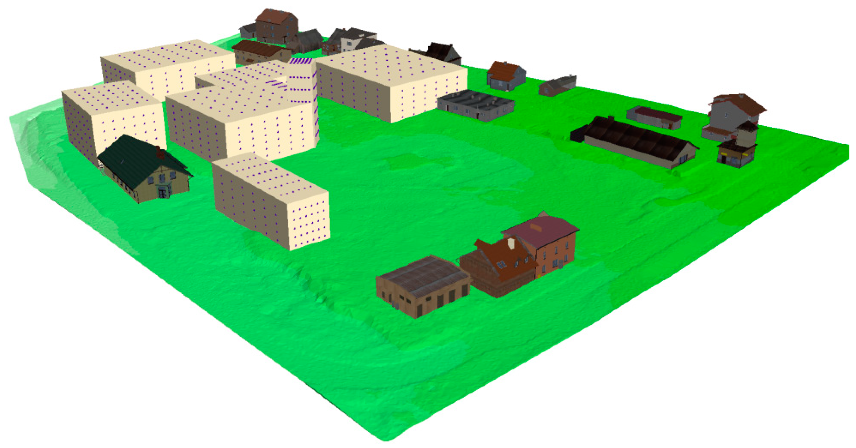
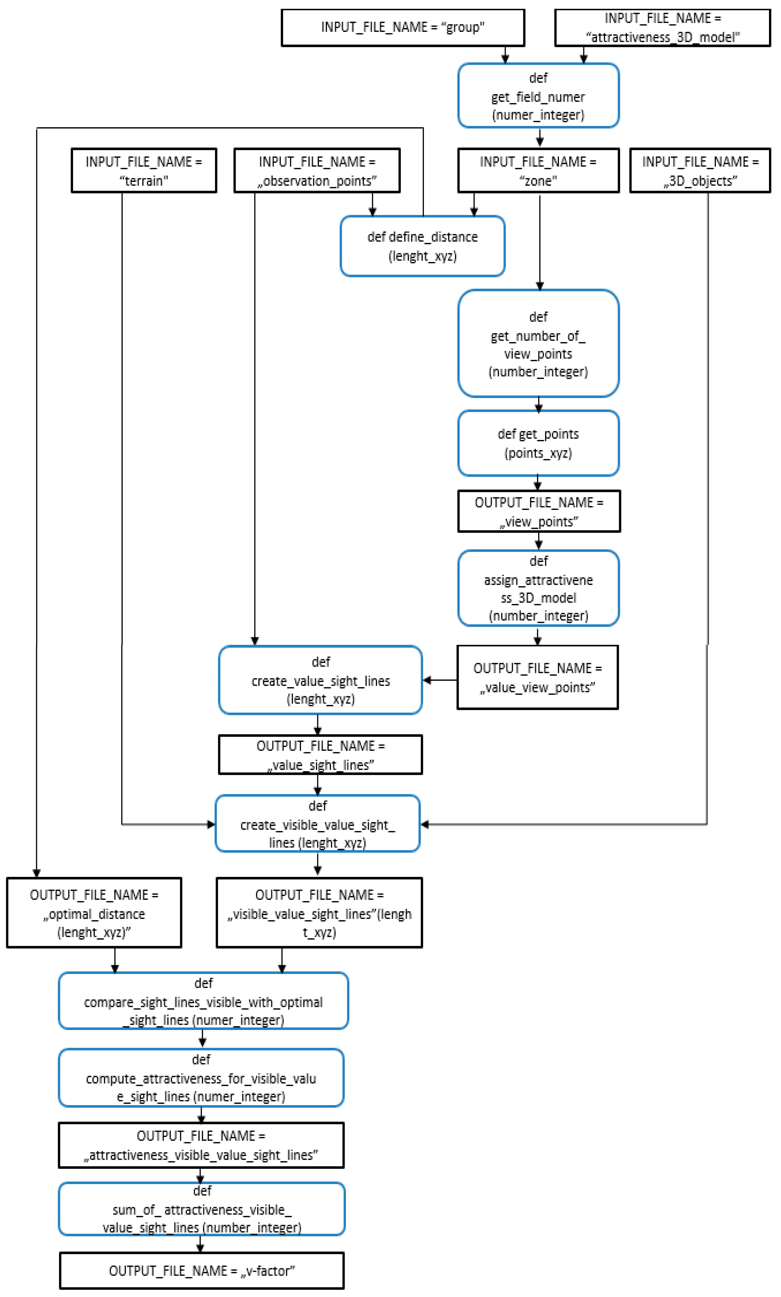
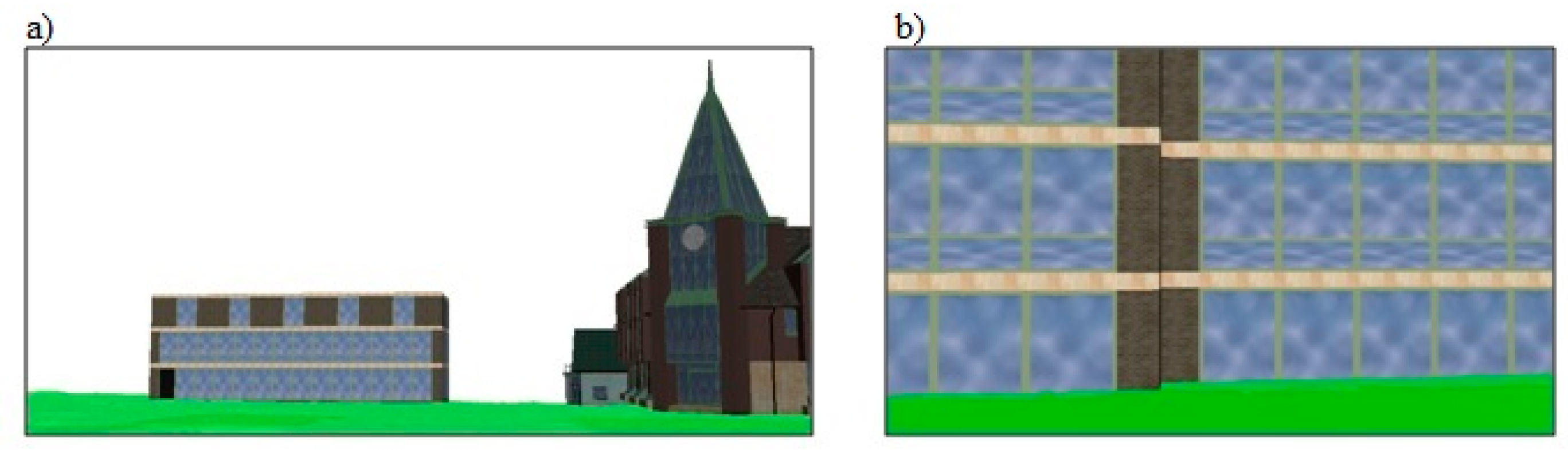
• ‘3D spatial model’—a set of 3D models of the existing buildings in the field and planned 3D objects in the studied area (Figure 3).
• ‘group’—the group can be a single-element group in the case of a 3D object of a spatial model with simple geometry or a multi-element group for complex geometries.
• ‘attractiveness_3D_model’—the attractiveness of an object of a 3D spatial model: a number (weight) from the set of integers, defined for the object of the 3D spatial model. The numerical values are assigned based on the Wejchert’s impression curve method. The assessment of the attractiveness of objects of a 3D spatial model uses an interactive visualisation of the 3D spatial model. The function of rotation, zooming in/out, and moving the 3D visualisation allows the user to explore the 3D spatial model in detail.
• ‘terrain’—a 3D representation of terrain surface.
• ‘observation_points’—the location and the number of observation points are defined in the three-dimensional space as necessary. For the purposes of defining the impact of buildings planned under the local development plan on the existing buildings in the area, it is advisable to set observation points in windows of the existing buildings [30].
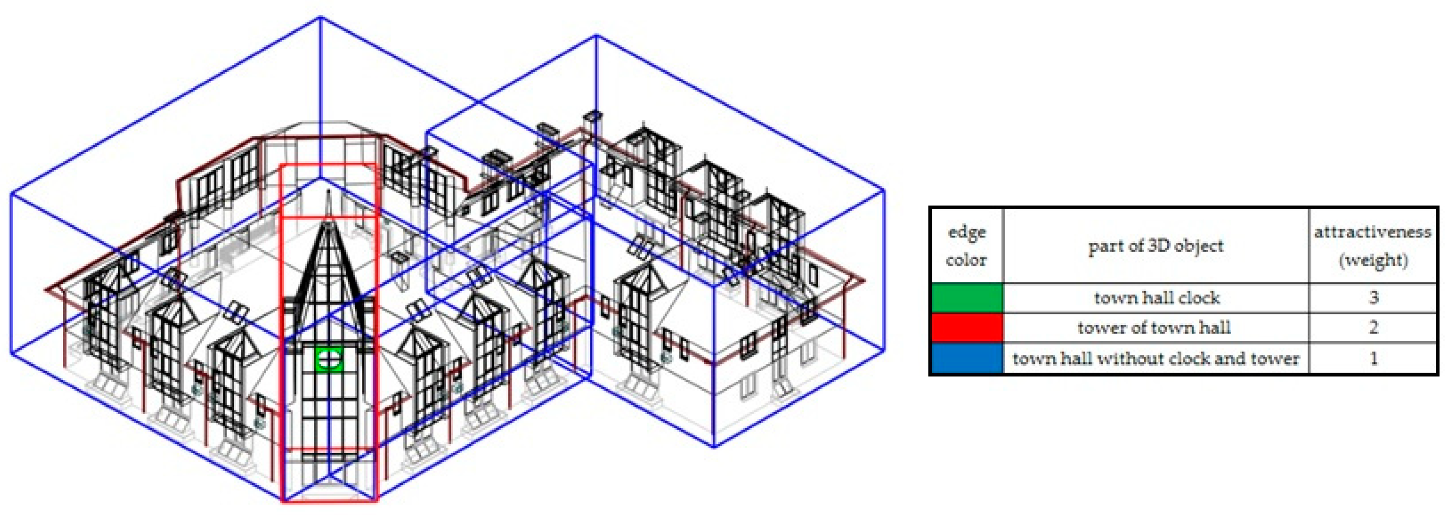
• ‘zone’—the smallest possible cuboid that contains a block of a 3D object. Its vertical edges are parallel to the Z axis of the Cartesian system adapted for the given object of the 3D spatial model (Figure 4).
  While determining the zones of visibility, it is necessary to describe the geometry of the 3D object with the smallest possible number of zones of visibility. In case the geometry of the 3D object is complex, the term ‘group’ is introduced. The zones of visibility belonging to the same group have the same attractiveness. The group can be a single-element group for 3D objects with simple geometry or a multiple-element group for objects with complex geometry. The decision on introducing a group is made by the user after analysing the geometry of the 3D object.
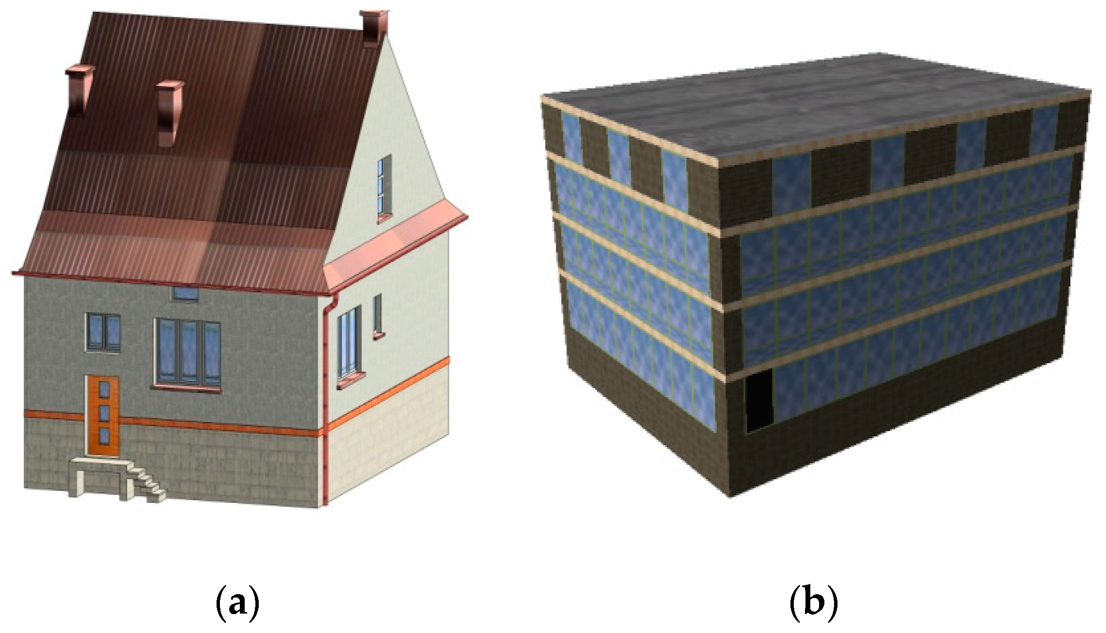
• ‘3D_objects’—a three-dimensional, approximate representation of each element of space that is the subject of the study. 3D objects designed as part of the local development plan.
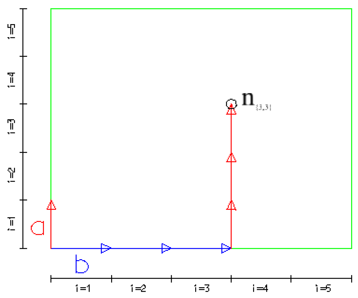
• ‘number_of_view_points’—the number of viewpoints (VPN) for the wall of the zone of visibility is constant for all walls of all zones of visibility present in a spatial model. The number of VPNs must be a square of an integer. For this purpose, two vectors were designed ($\overrightarrow{\mathrm{a}}$, $\overrightarrow{\mathrm{b}}$). Each of them is parallel to one of the two adjacent sides of the wall and their lengths are equal 1/n of the length of the respective sides where n = √(VPN) + 1. n{i,j} is a grid point where: i, j ∈ [1, √(VPN)] determined from the formula: n{i, j} = (i ∗ $\overrightarrow{\mathrm{a}}$ + j ∗ $\overrightarrow{\mathrm{b}}$) (Figure 5).
• ‘view_points’—a set of points where each point is located on the surface of the zone of visibility. Viewpoints are determined in such a way that they are located on the sides of the view wall and they are the vertices of rectangles dividing the wall into congruent rectangles whose vertices divide all sides of the wall into an equal number of segments. For a single-element group, the number of points of view for the wall of the zone of visibility is equal to VPN_single-el = VPN, while for a multi-element group VPN_multi-el. = VPN/n, where n equals the number of zones of visibility belonging to a given group. Introducing the term ‘VPN_multi-el.’ prevents an uneven contribution of a particular attractiveness of the zone of visibility to the result of the V-factor indicator.
• ‘value_view_point’ = numerical value (weight) is determined for each viewpoint. This is equal to the attractiveness of the zone of visibility to which the point belongs (Figure 6). Every viewpoint must have assigned the attractiveness of the zone of visibility to which it belongs.
• ‘value_sight_lines’—a segment connecting the observation point with the value viewpoint. Every sightline must have assigned the attractiveness of the value viewpoint corresponding to it.
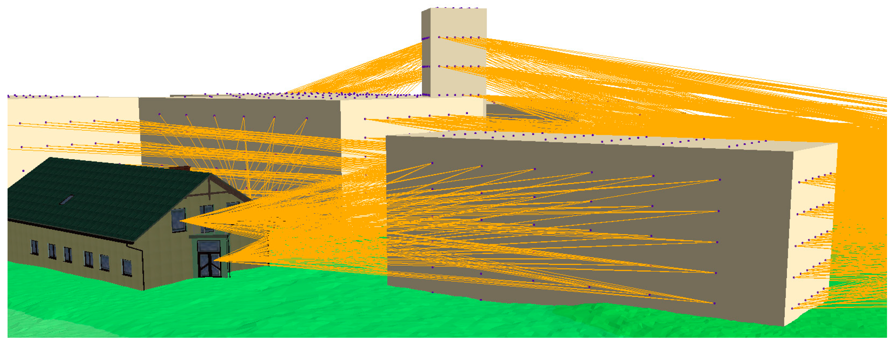
• ‘visible_value_sight_lines’—value sightline not crossing any 3D objects of the 3D spatial model (Figure 7).
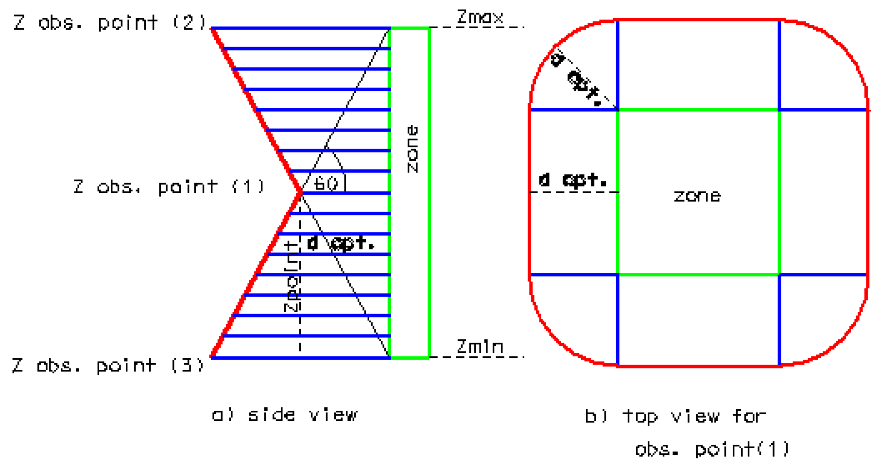
• ‘optimal_distance’—the distance between an observation point and the zone of visibility calculated for each zone of visibility defined for the 3D object of the 3D spatial model. The assumption was made that the optimal distance of observation is that at which the total height of the zone is visible from the observation point, assuming a vertical observer angle of 120 degrees. The total height of the 3D object of the 3D spatial model is calculated as the difference between the Z coordinate of the upper and lower base of the zone of visibility assigned to each 3D object of the 3D spatial model (Figure 8).

  d_opt. = ((Z_max − Z_min) − Z_obs) ∗ ctgφ

  (1)
• ‘attractiveness_visible_value_sight_lines’ – the attractiveness of the sightline is determined for each sightline based on the following formula:

Case 1: length of the sightline ˂ optimal observation distance:

$$\frac{[\sin \left(\alpha \right)\ast A+\cos \left(\beta \right)\ast A]\ast d}{d_0}$$

(2)

Case 2: length of the sightline ≥ optimal observation distance:

$$\frac{[\sin \left(\alpha \right)\ast A+\cos \left(\beta \right)\ast A]\ast d_0}{d}$$

(3)

where:

• $\alpha$—the horizontal angle between the sightline and the zone of visibility it falls on,
• $\beta$—the vertical angle between the sightline and the zone of visibility it falls on,
• $A$—the attractiveness of the zone of visibility containing a view point that belongs to a given sightline,
• d—the length of the sightline,
• $d_0$—the optimal observation distance.

Angle $\alpha$ assumes values from the range from 0° to 180°. For the value of angle $\alpha$ equal to 90°, the sightline falls at a right angle on the wall of visibility in the location of an appropriate view point.

Angle $\beta$ assumes values from the range from –90° to +90°. For the value of angle $\beta$ equal to 0°, the sightline falls at a right angle on the wall of visibility in the location of an appropriate view point

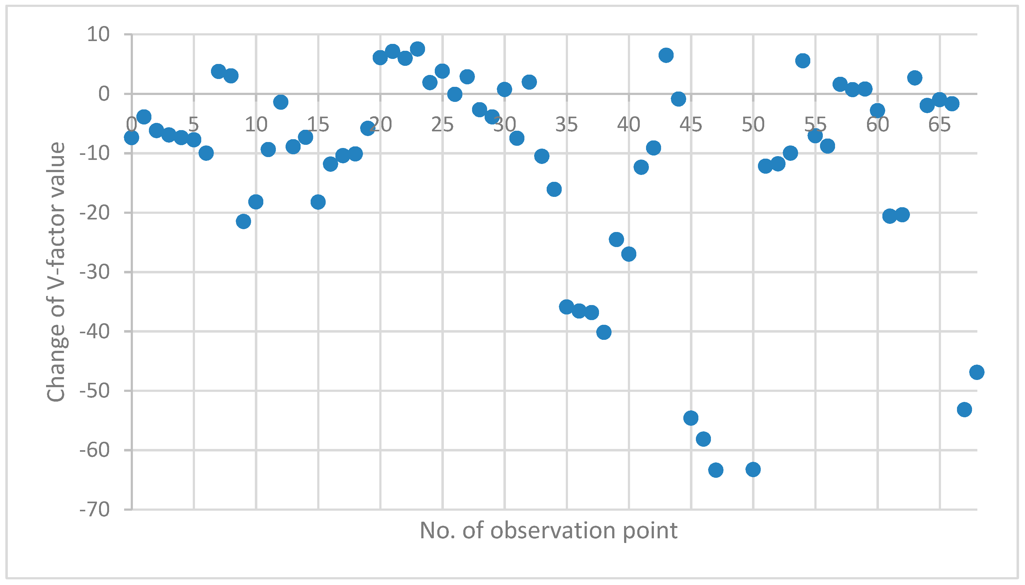
• ‘v-factor’—a sum of the values of attractiveness_visible_value_sight_lines of the sightlines corresponding to a given observation point.

The purpose of the V-factor is to determine the numerical values for the observation points, facilitating a comparative assessment of the attractiveness of view available from the special points in space with the assumed diverse attractiveness of space using objects of a 3D spatial model. The V-factor analysis provides information on how attractive a view available from a selected observation point is, taking into account the distance of the observation point from the observed object, vertical and horizontal angle of observation, and the aesthetic value of the observed object. For each observation point computed based on the V-factor algorithm, a numerical value was determined for the implementation of planning scenario 1 and planning scenario 2. In the next step, the differences between numerical values were computed as a result of replacing scenario 1 with scenario 2, which facilitated determining which one is more beneficial in terms of shaping the attractiveness of view. The implementation of the V-factor is described below (Figure 9).

4. Results

The values of the V-factor indicator were determined for the studied area. The analysis was conducted for two scenarios of spatial development, labelled scenario 1, and scenario 2. The set of observation points for each planning scenario included the same observation points located in the centres of windows of selected 3D models of existing buildings, excluding the 3D model of the City Hall. The observation points were located in windows of residential buildings directly adjacent to the area regulated by the local development plan. The observation points for the town hall were deliberately not specified as it is a public object not inhabited permanently. For the purpose of the analysis, the city hall was classified as an existing object, but having a significant impact on the attractiveness of view.

The value of the V-factor indicator for observation points in scenario 1 and scenario 2 as well as the change of the attractiveness of the available view for observation points resulting from the implementation of scenario 2 instead of scenario 1 (Figure 10) were determined in the analysis. Based on the alteration of the V-factor indicator value calculated as an average for all observation points, it is concluded that the implementation of scenario 2 will reduce the attractiveness of the available view in the scale of the entire area of the development by 42.17%. The use of the V-factor indicator makes it possible to compare planning scenarios with each other in terms of the impact on the attractiveness of view for specific observation points (Figure 11).

5. Discussion

Spatial planning should aim, in particular, at rational space development [1]. This would make it possible to balance social and economic interests [5,6,41]. In the context of fulfilling the needs of the local community [3], the most important is spatial planning on the municipal level through local development plans. The use of GIS tools in the process of drafting local development plans facilitates complex spatial analysis with unambiguous results. The analysis of the change in the attractiveness of view, carried out as part of the study, is in line with the relevant issue of three-dimensional analysis of visibility [29,30,31]. Moreover, the proposed method of studying the change of the attractiveness of view with the use of the V-factor indicator facilitates a global analysis for the entire studied area, which is consistent with the assumptions of the visual magnitude method [10]. The limitation of the method may be the computation requirements. In the case of studies on large surfaces, it is suggested to use simplified 3D models of existing objects, which significantly affects the efficiency of the calculation process. The use of 3D models of buildings with the Level of Detail 3, with exact geometry of walls, roofs, and distinguishing elements such as chimneys, windows, and doors [19] in the V-factor analysis, facilitates objective results regarding the view attractiveness change for the observation points. Thus, it helps to select the most advantageous planning concept, maintaining the harmony of landscape and ecological balance [40].

Further research work is planned dedicated to the development of the algorithm for determining the V-factor indicator. It is proposed to include medium and high vegetation and additional anthropogenic objects that are not buildings in the V-factor algorithm. Additionally, it is planned to create a graphic user interface where the function could be activated from the user workspace. The further research work will be an extension of the subject introduced in the paper, contributing to the improvement of knowledge in the field of spatial planning.

6. Conclusions

With three-dimensional data integrated with two-dimensional data, it is possible to carry out the analysis of the change in the attractiveness of the available view for observation points (V-factor). Using its results, a more beneficial planning scenario can be identified. The V-factor indicator can be successfully used in the process of spatial planning, in particular at the stage of determining the parameters of new buildings and location of visibility lines. Obtaining one numerical value reflecting the attractiveness of view for each planning scenario facilitates their efficient comparison, which is important for choosing the most favourable scenario. The guiding principle in the process of preparing local development plans should be performing the V-factor analysis. In addition, the results of such an analysis should be made available during public consultations regarding spatial solutions in the local plan as it can significantly contribute to the improvement of the effectiveness of public participation in the process of spatial planning. Increasing the awareness of the local community regarding proposed spatial solutions designed in the local development plan corresponds to the assumptions of the Agenda for Sustainable Development, goal 11.3 [42]. Moreover, according to the assumptions of [42], universal access to safe, inclusive, and accessible green and public spaces should be provided, in particular for women and children, the elderly, and persons with disabilities. The V-factor analysis can be a valuable element of the decision-making process in the space development which fulfils the requirements set by the Agenda for Sustainable Development.

The method has a universal character and can be used also for other purposes in the domain of real estate management. The V-factor can also be used to assess the attractiveness of view for planned public, office, or residential buildings according to the local plan. Knowing the value of the V-factor indicator it is possible to establish the price of sale or rent of newly designed surfaces depending on the attractiveness of the available view, which is advantageous from the economic point of view.

References

- Adams, N.; Alden, J.; Harris, N. Regional Development and Spatial Planning in an Enlarged European Union; Routledge Taylor & Francis Group: New York, NY, USA, 2016; p. 5. [Google Scholar]
- Fountas, S.; Wulfsohn, D.; Blackmore, B.S.; Jacobsen, H.L.; Pederson, S.M. A model of decision-making and information flows for information-intensive agriculture. Agr. Syst. 2006, 87, 192–210. [Google Scholar] [CrossRef]
- Matsuoka, R.H.; Kaplan, R. People needs in the urban landscape: Analysis of Landscape and Urban Planning contributions. Landsc. Urban Plan. 2008, 84, 7–19. [Google Scholar] [CrossRef]
- Angelidou, M. Smart city policies: A spatial approach. Cities 2014, 41, S3–S11. [Google Scholar] [CrossRef]
- Zubizarreta, I.; Seravalli, A.; Arrizabalaga, S. Smart City Concept: What It Is and What It Should Be. J. Urban Plan. Dev. 2016, 142, 04015005. [Google Scholar] [CrossRef]
- Hernik, J.; Gawroński, K.; Dixon-Gough, R. Social and economic conflicts between cultural landscapes and rural communities in the English and Polish systems. Land Use Policy 2013, 30, 800–813. [Google Scholar] [CrossRef]
- Bishop, I.D.; Wherrett, J.R.; Miller, D.R. Assessment of path choices on a country walk using a virtual environment. Landsc. Urban Plan. 2001, 52, 225–237. [Google Scholar] [CrossRef]
- Pakzad, E.; Salari, N. Measuring sustainability of urban blocks: The case of Dowlatabad, Kermanshah city. Cities 2018, 75, 90–100. [Google Scholar] [CrossRef]
- Sabri, S.; Pettit, C.J.; Kalantari, M.; Rajabifard, A.; White, M.; Lade, O.; Ngo, T. What are Essential requirements in Planning for Future Cities using Open Data Infrastructures and 3D Data Models? In Proceedings of the CUPUM 2015, 14th International Conference on Computers in Urban Planning and Urban Management, Cambridge, MA, USA, 7–10 July 2015; Available online: https://www.opengeospatial.org/standards/citygml (accessed on 10 February 2019).
- Chamberlain, B.C.; Meitner, M.J. A route-based visibility analysis for landscape management. Landsc. Urban Plan. 2013, 111, 13–24. [Google Scholar] [CrossRef]
- Lippold, A. 3D city-scale modelling applied to sustainable design: history, example, and the future. In Proceedings of the policy conference, Stuttgart, Germany, 15–17 September 2010. [Google Scholar]
- Open Geospatial Consortium. Available online: https://www.opengeospatial.org/standards/citygml (accessed on 10 December 2018).
- Gröger, G.; Plümer, L. CityGML–Interoperable semantic 3D city models. ISPRS J. Photogramm. Remote Sens. 2012, 71, 12–33. [Google Scholar] [CrossRef]
- Catita, C.; Redweik, P.; Pereira, J.; Brito, M.C. Extending solar potential analysis in buildings to vertical facades. Comput. Geosci. 2014, 66, 1–12. [Google Scholar] [CrossRef]
- Chun, B.; Guldmann, J.M. Spatial statistical analysis and simulation of the urban heat island in high-density central cities. Landsc. Urban Plan. 2014, 125, 76–88. [Google Scholar] [CrossRef]
- Martínez, J.; Soria-Medina, A.; Arias, P.; Buffara-Antunes, F. Automatic processing of Terrestrial Laser Scanning data of building facades. Autom. Constr. 2012, 22, 298–305. [Google Scholar] [CrossRef]
- Pu, S.; Vosselman, G. Automatic extraction of building features from terrestrial laser scanning. Int. Arch. Photogramm. Remote Sens. Spat. Inf. Sci. 2006, 36, 25–27. [Google Scholar]
- Pu, S. Generating building outlines from terrestrial laser scanning. In Proceedings of the International Archives of the Photogrammetry, Remote Sensing and Spatial Information Sciences—Beijing, Part B5, XXXVII, Beijing, China, 3–11 July 2008. [Google Scholar]
- Pluta, M.; Głowacka, A. Dokładność modelowania 3D na podstawie chmury punktów z naziemnego skaningu laserowego. Episteme Czasopismo Kulturalno Naukowe 2015, 26, 125–132. [Google Scholar]
- Jim, C.; Chen, W.Y. Impacts of urban environmental elements on residential housing prices in Guangzhou (China). Landsc. Urban Plan. 2006, 78, 422–434. [Google Scholar] [CrossRef]
- Suleiman, W.; Joliveau, T.; Favier, E. 3D Urban Visibility Analysis with vector Gis Data. In Proceedings of the 19th annual GIS Research UK (GISRUK), University of Portsmouth, Portsmouth, UK, 27–29 April 2011. [Google Scholar]
- Miller, D. A method for estimating changes in the visibility of land cover. Landsc. Urban Plan. 2001, 54, 93–106. [Google Scholar] [CrossRef]
- Turner, A.; Doxa, M.; Sullivan, D.; Penn, A. From isovists to visibility graphs: a methodology for the analysis of architectural space. Environ. Plann. B Plann. Des. 2001, 28, 103–121. [Google Scholar] [CrossRef]
- Albrecht, F.; Moser, J.; Hijazi, I. Assessing facade visibility in 3d city models for city marketing. In Proceedings of the ISPRS 8th 3D GeoInfo Conference & WG II/2 Workshop, XL-2/W2, Istanbul, Turkey, 27–29 November 2013. [Google Scholar]
- Davidson, D.; Watson, A.; Selman, P. An evaluation of GIS as an aid to the planning of proposed developments in rural areas. Geogr. Inf. Handl. Res. Appl. 1993, 1, 251–259. [Google Scholar]
- Iverson, W. And that’s about the size of it: Visual magnitude as a measurement of the physical landscape. Landsc. J. 1985, 4, 14. [Google Scholar] [CrossRef]
- Benedikt, M.L. To take hold of space: isovists and isovist fields. Environ. Plann. 1979, 6, 47–65. [Google Scholar] [CrossRef]
- Bartie, P.; Reitsma, F.; Kingham, S.; Mills, S. Advancing visibility modelling algorithms for urban environments. Comput. Environ. Urban Syst. 2010, 34, 518–531. [Google Scholar] [CrossRef]
- Chmielewski, S.; Tompalski, P. Estimating outdoor advertising media visibility with voxel-based approach. Appl. Geogr. 2017, 87, 1–13. [Google Scholar] [CrossRef]
- Fisher-Gewirtzman, D.; Shashkov, A.; Doytsher, Y. Voxel based volumetric visibility analysis of urban environments. Surv. Rev. 2013, 45, 451–461. [Google Scholar] [CrossRef]
- Feng, W.; Gang, W.; Deji, P.; Yuan, L.; Liuzhong, L.; Hongbo, W. A parallel algorithm for viewshed analysis in three-dimensional Digital Earth. Comput. Geosci. 2015, 75, 57–65. [Google Scholar] [CrossRef]
- Suleiman, W.; Joliveau, T.; Favier, E. Advances in Spatial Data Handling; Springer: Berlin/Heidelberg, Germany, 2013; pp. 157–173. [Google Scholar]
- Bartie, P.; Mackaness, W. Mapping the visual magnitude of popular tourist sites in Edinburgh city. J. Maps 2016, 12, 203–210. [Google Scholar] [CrossRef]
- Sawada, M.; Cossette, D.; Wellar, B.; Kurt, T. Analysis of the urban/rural broadband divide in Canada: Using GIS in planning terrestrial wireless deployment. Gov Inf. Q. 2006, 23, 454–479. [Google Scholar] [CrossRef]
- Guneya, C.; Girginkaya, S.A.; Cagdas, G.; Yavuz, S. Tailoring a geomodel for analyzing an urban skyline. Landsc. Urban Plan. 2012, 105, 160–173. [Google Scholar] [CrossRef]
- Karimimoshaver, M.; Winkemann, P. A framework for assessing tall buildings’ impact on the city skyline: Aesthetic, visibility, and meaning dimensions. Environ. Impact Asses. Rev. 2018, 73, 164–176. [Google Scholar] [CrossRef]
- Rafieian, M.; Rad, H.R.; Sharifi, A. The Necessity of using Sky View Factor in Urban Planning: A Case Study of Narmak Neighborhood, Tehran. In Proceedings of the 2014 International Conference and Utility Exhibition on Green Energy for Sustainable Development (ICUE 2014), Pattaya City, Thailand, 19–21 March 2014. [Google Scholar]
- Yang, F.; Qian, F.; Lau, S. Urban form and density as indicators for summertime outdoor ventilation potential: A case study on high-rise housing in Shanghai. Build. Environ. 2013, 70, 122–137. [Google Scholar] [CrossRef]
- Oh, K. Visual threshold carrying capacity (VTCC) in urban landscape management: A case study of Seoul, Korea. Landsc. Urban Plan. 1998, 39, 283–294. [Google Scholar] [CrossRef]
- Kupidura, A.; Bielska, A.; Rogoziński, R. Analiza i ocena krajobrazu wizualnego wsi na potrzeby opracowania planów rozwoju obszarów wiejskich. Studia Komitetu Przestrzennego Zagospodarowania Kraju PAN 2012, 1, 336–342. [Google Scholar]
- Lai, S.-K. Why plans matter for cities. Cities 2018, 73, 91–95. [Google Scholar]
- Sustainable Development Goals Knowledge Platform. Available online: https://sustainabledevelopment.un.org/post2015/transformingourworld (accessed on 10 February 2019).
© 2019 by the authors. Licensee MDPI, Basel, Switzerland. This article is an open access article distributed under the terms and conditions of the Creative Commons Attribution (CC BY) license (http://creativecommons.org/licenses/by/4.0/).
Share and Cite
Pluta, M.; Mitka, B. V-Factor Indicator in the Assessment of the Change in the Attractiveness of View as a Result of the Implementation of a Specific Planning Scenario. ISPRS Int. J. Geo-Inf. 2019, 8, 78. https://doi.org/10.3390/ijgi8020078
Pluta M, Mitka B. V-Factor Indicator in the Assessment of the Change in the Attractiveness of View as a Result of the Implementation of a Specific Planning Scenario. ISPRS International Journal of Geo-Information. 2019; 8(2):78. https://doi.org/10.3390/ijgi8020078
Chicago/Turabian StylePluta, Magda, and Bartosz Mitka. 2019. "V-Factor Indicator in the Assessment of the Change in the Attractiveness of View as a Result of the Implementation of a Specific Planning Scenario" ISPRS International Journal of Geo-Information 8, no. 2: 78. https://doi.org/10.3390/ijgi8020078
APA StylePluta, M., & Mitka, B. (2019). V-Factor Indicator in the Assessment of the Change in the Attractiveness of View as a Result of the Implementation of a Specific Planning Scenario. ISPRS International Journal of Geo-Information, 8(2), 78. https://doi.org/10.3390/ijgi8020078