Abstract
The Geographic Object-Based Image Analysis (GEOBIA) paradigm relies strongly on the segmentation concept, i.e., partitioning of an image into regions or objects that are then further analyzed. Segmentation is a critical step, for which a wide range of methods, parameters and input data are available. To reduce the sensitivity of the GEOBIA process to the segmentation step, here we consider that a set of segmentation maps can be derived from remote sensing data. Inspired by the ensemble paradigm that combines multiple weak classifiers to build a strong one, we propose a novel framework for combining multiple segmentation maps. The combination leads to a fine-grained partition of segments (super-pixels) that is built by intersecting individual input partitions, and each segment is assigned a segmentation confidence score that relates directly to the local consensus between the different segmentation maps. Furthermore, each input segmentation can be assigned some local or global quality score based on expert assessment or automatic analysis. These scores are then taken into account when computing the confidence map that results from the combination of the segmentation processes. This means the process is less affected by incorrect segmentation inputs either at the local scale of a region, or at the global scale of a map. In contrast to related works, the proposed framework is fully generic and does not rely on specific input data to drive the combination process. We assess its relevance through experiments conducted on ISPRS 2D Semantic Labeling. Results show that the confidence map provides valuable information that can be produced when combining segmentations, and fusion at the object level is competitive w.r.t. fusion at the pixel or decision level.
1. Introduction
The Geographic Object-Based Image Analysis (GEOBIA) paradigm has become very popular for processing aerial and satellite imagery [1,2,3]. It relies strongly on the segmentation concept, i.e., partitioning of an image into regions or objects that are then further analyzed (e.g., described and classified) [4,5]. Choosing an appropriate scale for the segmentation step is challenging and has been the subject of extensive studies [6,7,8,9,10]. Despite these efforts, finding a perfect segmentation is an ill-posed problem, and there is no (and probably will never be) a universal, domain- and image-independent segmentation technique [1]. To produce a segmentation from some remotely-sensed observations of a scene, various criteria have to be taken into account, namely the homogeneity of the scene and the size of the objects, the properties of the input image (e.g., its spatial resolution), the method of segmentation and its parameter settings (including the segmentation criteria, the scale, etc.). If multiple sensors or multi-temporal data are used, the segmentation process can exploit multiple sources of information to create the objects.
Applying a GEOBIA process to multiple data sources requires fusing or combining information at certain stages [11,12,13]. Such a task can be performed at different stages of the overall process: (i) before segmentation, by merging the input data into one single, possibly multi-valued image (i.e., fusion at pixel level; [13]); such an image will then be segmented, leading to a single segmentation map that is then classified; (ii) after segmentation but before classification, by combining multiple segmentations into a single one that will serve as a support for the classification process (i.e., fusion at object level; [14]); (iii) after classification, by merging the decisions taken by the multiple classifiers, each of which is specific to a segmentation input (i.e., fusion at decision level; [15]). While the first strategy greatly reduces the richness of the information by providing a single image as input to the segmentation, the third strategy leads to multiple, inconsistent classification maps since there is no guarantee that the objects classified in the different segmentation maps have the same spatial support. In this paper, we explore the second strategy, i.e., combining multiple segmentations into a single one that is used as an input for the subsequent classification stage.
We present a generic framework to combine multiple segmentation maps into a fine-grained partition of segments (super-pixels or small-size pixels, i.e., connected sets of similar pixels obtained from an over-segmentation process) that is built by intersecting individual input partitions. Each segment is then attributed a segmentation confidence score that directly relates to the consensus between the different individual segmentation inputs concerning this segment. We discuss how such a score can be exploited in further processing, beyond its direct use to produce a unique segmentation. Further, we show how to adapt it to allow an expert to input prior knowledge through local or global weights attached to specific regions or images, respectively.
The rest of the paper is organized as follows. First we review existing approaches for the combination of segmentations in Section 2 and explain how our work differs from the state-of-the-art. In Section 3, we present our general framework, the confidence score, the expert priors, and discuss possible ways to exploit the confidence map. In Section 4 we describe the experiments, including the dataset, parameter settings, and the results we obtained with partial and full segmentation, as well comparing our strategy with other fusion strategies. In Section 5 we present our conclusions and future research directions.
2. Related Works
Combining multiple, possibly contradictory segmentations is not simple. Indeed, segmentation is an ill-posed problem and no perfect generic segmentation method or parameter settings are suitable for use in all situations. So the problem of combining multiple segmentations to find an optimal partition has received considerable attention and various methods have been proposed, usually in the form of modeling input segmentations as region adjacency graphs (RAG) [14] and careful analysis of similarities between neighboring regions in order to identify the unitary regions that need to be merged into larger ones. In [16], a general framework is proposed to combine multiple segmentations of a single image by generating and filtering super-pixels, building multiple clusterings of super-pixels and identifying a consensus clustering from which a single segmentation is derived. Among the optimization schemes, Markov Random Fields (MRF) have been used to embed global priors (e.g., related to the number of regions expected in the output segmentation) [17] while a bag of super-pixels has been analyzed in [18] using bipartite graph clustering.
However, most of these methods rely to a great extent on the raw features (e.g., color, texture) provided by an input image to drive the combination process, or at least they assume a single input image from which multiple segmentations are derived. Most of these input segmentations are obtained by considering color images, usually using various parameter settings of the same segmentation method, e.g., RAG in [14], Texture and Boundary Encoding-based Segmentation (TBES) and/or Ultrametric Contour Map (UCM) in [16], Mean-Shift and Felzenszwalb in [18]. Transformation of the color image into different color spaces before applying K-Means clustering was used in [17]. If the input segmentations come from very different input data (different dates, sources or modalities) and not only from different methods applied over the same input image, priority could go to some segmentations in the combination process, since the inputs are not necessarily equally reliable.
To obtain extractions from optical remote sensing images [19], multiple segmentations are used to extract vegetation, shadow and rectangular areas. These segmentations are then merged using MRF over the RAG, considering the co-occurrence of adjacent segments and color features in the optimization process. Other examples of processing multispectral images include [20,21] who propose respectively an unsupervised and semi-supervised framework to find an optimized segmentation in a single remotely-sensed image to use as input.
The fusion of multiple segmentations has been widely addressed in the field of computer vision, through coclustering [22] or cosegmentation [23]. However, these methods assume the input images contain one (or a few) foreground objects over a background, which does not correspond to the contents of remote sensing data. Expert knowledge can be exploited in interactive frameworks when the user scribbles over the foreground and background [24].
Among the methods that do not depend on the input data is a recent approach reported in [25] in which several multiscale segmentations are combined into one. More precisely, the authors consider each input multiscale segmentation as a binary partition tree structure in which pairs of the most similar regions are iteratively merged. The initial regions are the same for all trees and a majority vote procedure makes it possible to derive a single merging sequence (and hence multiscale segmentation) from these multiple series. While this approach does not make any assumption concerning the input data, it is limited to input segmentations obtained using a binary partition tree, and is not suitable for the wide range of segmentation techniques that are available.
In contrast to existing methods that rely on the original data (before segmentation) to combine the multiple segmentation maps, we propose a simple generic framework that considers only segmentation maps. This makes sense particularly when the maps are the result of different input data, with no prior knowledge of the kind of data sources that fed the combination process. Indeed, in the context of remote sensing, when combining multiple sources (e.g., LiDAR, optical imagery, SAR, etc.) or multiple dates, it is not always possible to determine a priori the underlying criterion (e.g., color, elevation) to fuse input maps. While the proposed framework is fully unsupervised, since it is based only on local consensus between segmentations, we still allow the expert to input prior knowledge through a weighting scheme that can be applied globally or locally. Finally, we discuss how to deal with the consensus score beyond its direct use to derive a unique segmentation result.
3. Method
As mentioned in the introduction, our goal is to build an optimal segmentation map from a set of inputs. Our method is not a segmentation technique per se, but rather aims to merge existing segmentation maps. Such maps can be derived from various data sources (e.g., optical images and DSM), various dates, various segmentation techniques (e.g., thresholding, edge-based and region-based techniques), and defined from various parameter settings, as shown in Figure 1. In the following subsections, we describe the general framework and discuss the confidence measure, the integration of prior knowledge, and the possible use of the confidence map that is the output of our combination framework.
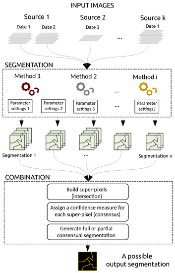
Figure 1.
Our generic framework to combine multiple segmentations in the GEOBIA paradigm. Segmentations can come from different data sources (e.g., optical and radar sensors) and be acquired at different dates. They may also be produced using different methods (e.g., region-based or edge-based) relying on different parameter values.
3.1. Overall Framework
The proposed framework for combining prior segmentations comprises the four following steps:
- build the initial segmentations (multiple sources, methods and parameters);
- build a very fine partition by intersecting the input segmentations;
- assign a confidence measure to each region;
- use the confidence map to build a consensual result.
Steps 1 and 2 are straightforward and consist in building a single oversegmentation map made of super-pixels generated from an initial segmentation ensemble. At this stage, we do not make any assumptions concerning the coherence between the different input segmentations that may originate from different images/sources/dates (here we assume no changes in the scene between the different dates; otherwise we can use the confidence score to detect any changes, see discussion in Section 3.2), different methods or settings, that could lead to conflicting segments. We only assume these input segmentations share the same spatial resolution and coverage footprint. This is required to extract intersecting super-pixels. If this condition is not fulfilled, a resampling step is applied to ensure all segmentations are spatially comparable. Overlapping segments are then merged following the most restrictive strategy: adjacent pixels are combined in the same super-pixel if and only if they belong to the same segment in all the input segmentation maps.
3.2. Confidence Measure
Super-pixels are generated by intersecting all the segmentations that are fed to the framework. To illustrate this process, Figure 2a–f shows some sample segmentations built from an input satellite image (Pleiades multispectral image, Figure 2g). Figure 2h illustrates the resulting oversegmentation built by intersecting the input maps. The combination framework proposed here makes it possible to derive a confidence value for each super-pixel, as shown in Figure 2i.
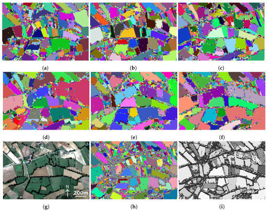
Figure 2.
From input segmentations to confidence map: input segmentations (a–f) extracted from a single data source (g), their intersection into super-pixels (h) and the resulting confidence value map (i). Pseudo-colors are randomly generated from region labels providing one different color per region. In the confidence value map, brighter color corresponds to a higher confidence score, and darker color indicates a lower confidence score. The single data source (g) was extracted from an optical Pleiades multispectral image acquired on 12 October 2013.
The confidence measure is a core element of our framework. We rely on the measures proposed by Martin [26] that were used to evaluate results in the well-known Berkeley Segmentation Dataset. Such measures have recently been used in an optimization scheme for segmentation fusion [17]. First we recall the definitions provided in [26], before defining the confidence measure used in this paper.
Let us first consider two input segmentations and . Writing the set of pixels in segmentation S that are in the same segment as pixel p, we can measure the local refinement error in each pixel p of the image space through the following equation:
where denotes cardinality and set difference. Since this measure is not symmetric, Martin proposed several global symmetric measures: the Local Consistency Error (LCE), the Global Consistency Error (GCE), the Bidirectional Consistency Error (BCE) respectively computed as
and
The latter has been further extended considering a leave-one-out strategy, leading to
and we rely on this idea in our proposal, as described further on in this section. Let us recall that these measures were not used to merge segmentations, as a variant using an average operator is proposed in [17] to achieve this goal:
In contrast to previous metrics, we consider the scale of super-pixels. Consequently, we assign a score to each super-pixel that measures the degree of consensus between the different input segmentations in the same super-pixel. denotes the set of m input segmentations, from which we derive a single set of n super-pixels defined as . Each super-pixel is obtained by intersecting the input segmentations, i.e., two pixels p and q are in the same super-pixel if and only if . In order to counter the directional effect of the local refinement error at the pixel scale, we propose the following measure:
In other words, we measure the ratio of the smaller region that does not intersect (or is not included in) the larger region. It differs considerably from the bidirectional definitions given in [17,26] that do not distinguish between each pair or regions.
Since our goal is not to aggregate this error at the global scale of an image like with (or a pair of images with , , , ), but rather to measure a consistency error for each super-pixel, we define the Super-pixel Consistency Error as:
that is by definition equal for all , so we simply write instead of . Since our revised local refinement error is bidirectional in (7), we can add the constraint in (8) to reduce computation time. Finally we define the confidence value of each super-pixel with . Furthermore, the computation is limited to super-pixels instead of to the original pixels, leading to an efficient algorithm. For the sake of comparison, we recall that the maximum operator in (8) was replaced by an average operator at the image scale in [17].
Our framework assigns a high confidence value when the regions that make up a super-pixel resemble each other, and a low confidence value in the case of locally conflicting segmentations, as shown in Figure 2i. The figure shows that such conflicts appear mostly at the edges of the super-pixels, since these parts of the image are more likely to change between different segmentations. A more comprehensive close-up is provided in Figure 3, in which three different scenarios to combine six segmentations Figure 3a are compared. For the sake of visibility, a single object is considered and the overlapping segments in the input segmentations are provided. In the first case Figure 3b, all the regions share a very similar spatial support and the confidence in the intersecting super-pixel is consequently high. Conversely, there is a notable mismatch between overlapping regions in Figure 3c, leading to a low confidence score. Finally, we avoid penalizing nested segmentations such as those observed in Figure 3d, thanks to our definition of the local refinement error (7) that focuses on the ratio of the smaller region that does not belong to the larger one.
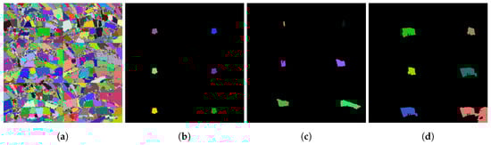
Figure 3.
Different consensus scenarios: (a) input segmentations (left and right), (b) high confidence (consensus between regions of the two segmentations), (c) low confidence (mismatch between regions), (d) high confidence (regions are nested within others). Pseudo-colors are randomly generated from region labels providing one different color per region.
By relying on the consensus between the different input segmentation maps, our combination framework provides a single feature when dealing with multiple dates as inputs. Indeed, in a change detection context, high confidence will be assigned to stable regions (i.e., regions that are not affected by changes) since they correspond to agreements between the different inputs. Conversely, areas of change will lead to conflicts between the input segmentations and thus will be characterized by a low confidence score. The (inverted) confidence map could then be used as an indicator of change, but this possibility is left for future work.
3.3. Prior Knowledge
In the GEOBIA framework, expert knowledge is often defined through rulesets, selection of relevant attributes or input data. Here, we consider that while the framework might be fed with many input segmentations, some prior knowledge about the quality of such segmentations may be available and is worth using.
More precisely, it is possible to assess the quality of the segmentation at two different levels. On the one hand, a user can assign a confidence score to a full segmentation map. This happens in some cases where specific input data (or a set of parameters) do not provide accurate segmentation (e.g., a satellite image acquired at a date when different land cover cannot be clearly distinguished or the image has a high cloud cover). Conversely, there are situations in which we can assume that a given segmentation will produce better results than others, e.g., due to a higher spatial resolution (i.e., a level of detail that fit the targeted objects) or a more relevant source (e.g., height from nDSM is known to be better than spectral information to distinguish between buildings and roads). In both cases, the weight remains constant for all the regions of a segmentation.
On the other hand, such confidence can be determined locally. Indeed, it is possible that a segmentation is accurate for some regions and inaccurate for others. In this case, the user is able to weight specific regions of each input, either to express confidence in the region considered or to identify regions of low quality. Note that the quality assessment could originate either from the geographical area (e.g., the presence of relief) or from the image segments themselves.
In order to embed such priors in the combination framework, we simply update our local refinement error defined in (7):
with denoting the weight given to , i.e., the segment of S containing p. If the prior is defined locally, then two pixels belonging to the same region in S will have the same weight, i.e., . If it is defined globally, then it is shared among all pixels of the image . By default, we set , and only expert priors change the standard behavior of the framework. If one region or one image is given high confidence, then its contribution to local refinement error will be higher, and it will thus have a strong effect on the super-pixel consistency error (the region lacks consensus with other regions). Conversely, if one region or image is given low confidence, then the local refinement error will be low, and the region/image will not drive the computation of the super-pixel consistency error. Since the local refinement error compares two individual regions, we include both related weights in the computation (while still keeping a symmetric measure). Finally, note that while all measures discussed in Section 3.2 are defined in , the weighting by leads to confidence measures also defined on . A normalization step is required before computation of the confidence map to insure it remains in . When illustrating the confidence map in this paper, we consider only the unweighted version and rescale it into gray levels.
From a practical point of view, assigning weights to prioritize some segmentation maps or some regions in a segmentation is an empirical task that relies on heuristics (knowledge of data and metadata, knowledge of the study site, expertise on segmentation algorithms). The pairwise comparison matrix inspired by the Analytical Hierarchy Process [27] is one way to rank criteria related to segmentations (data source, date, method, parameters) and to define quantitative weights.
3.4. Using the Confidence Map
We have presented a generic framework that is able to combine different segmentations and derive a confidence score for each super-pixel. Here we discuss how the confidence score can be further used to perform image segmentation, and we distinguish between partial and full segmentation.
3.4.1. Partial Segmentation
Let us recall that in each super-pixel, the confidence map measures the level of consensus between the different input segmentations. Super-pixels with a high confidence level most likely represent robust elements in the segmentation map, and thus need to be preserved. Conversely, super-pixels with a low confidence level denote areas of the image where the input segmentations do not match. Such regions could be reasonably filtered out by applying a threshold ( in Equation (10)) on the confidence map. Figure 4 illustrates the effect of confidence thresholding with various thresholds, as follows:
where super-pixels with confidence lower levels than are discarded (shown in black).
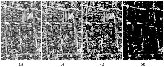
Figure 4.
An illustration of the confidence map (a) and the subsequent partial segmentation obtained with a threshold of (b) , (c) , and (d) . The brighter tone corresponds to higher confidence, and darker tone to lower confidence.
This process leads to partial segmentation, which provides only super-pixels for which the consensus was high. All the regions in the image that correspond to some mismatch between the input segmentations are removed and assigned to the background. This strategy is useful when the subsequent steps of the GEOBIA process have to be conducted on the significant objects only (here defined as those leading to a consensus between the input segmentations).
3.4.2. Full Segmentation
In order to obtain a full segmentation from the partial segmentation discussed above, background pixels have to be assigned to some of the preserved super-pixels. Several strategies can be used.
For instance, it is possible to merge each low-confidence super-pixel with its most similar neighbor. However this requires defining an appropriate criterion to measure the so-called similarity. While the similarity might rely on the analysis of the input data, it can also remain independent of the original data by assigning each low-confidence super-pixel to the neighbor with the highest confidence, or with which it shares the most border. Note that if a discarded super-pixel is surrounded by other super-pixels whose confidence levels are also below the threshold, the neighborhood has to be extended.
More advanced filtering and merging methods are reported in the literature [28], such as region growing on a region adjacency graph of super-pixels (called quasi-flat zones in [28]). Filtering is then based on the confidence of super-pixels rather than on their size. The growing process in [28] requires describing each super-pixel by its average color. Any of the available data sources can be used, leading to a process that is not fully independent of the input data (note that such input data are only used to reassign the areas of the image where the consensus is low, not to process the complete image). Otherwise, geometric or confidence criteria can be used.
Figure 5c highlights the super-pixels with low confidence levels (shown in white) that have to be removed and merged with the remaining ones (shown in black). As might have been expected, super-pixels in which input segmentations disagree actually correspond to object borders Figure 5b. Such areas are known to be difficult to process. Indeed, most of the publicly available contests in remote sensing apply specific evaluation measures to tackle this issue, e.g., eroding the ground truth by a few pixels to prevent penalizing the submitted semantic segmentation or classification map with inaccurate borders.
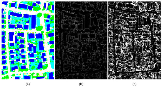
Figure 5.
Object borders are characterized with low confidence: (a) reference segmentation map, (b) borders of the reference objects, and (c) super-pixels with low-confidence.
Finally, it is also possible to retain all super-pixels but to use their confidence score in a subsequent process. In the context of geographic object-based image analysis, such a process might consist of a fuzzy classification scheme, in which the contribution of the super-pixel samples in the training of a prediction model will be weighted by their confidence. Since the focus of this paper is on the combination of segmentations and not their subsequent use, we do not explore this strategy further here, but we do include some preliminary assessments in the following section.
4. Experiments
Here we report several experiments conducted on the ISPRS 2D Semantic Labeling dataset to assess the relevance of the proposed generic framework for the combination of segmentations. The dataset is provided for the purpose of classification. In our GEOBIA context, we will thus evaluate our framework in terms of its ability to provide objects relevant for the subsequent classification. We first present the dataset and explain how we built the input segmentations, before presenting and discussing the results obtained for partial and full segmentation.
4.1. Dataset and Experimental Setup
In this paper, we consider one of the 2D Semantic Labeling Contest datasets [29], the Vaihingen region in Germany. The dataset contains a true color orthophoto (with red (R), green (G), and near infrared (NIR) channels) acquired with a ground resolution of 9 cm, as well as a Digital Surface Model (DSM) generated by interpolating the point clouds acquired by an airborne laser scanner (Leica ALS50 system) of the same region.
To complete the original data, like many other authors, we compute nDSM (normalized DSM) by subtracting DTM (Digital Terrain Model) from DSM. DTM is derived from DSM using progressive morphological filtering [30]. We then obtain nDSM, which stores information on the height of each pixel above the estimated ground. We also extract the popular NDVI feature computed from Near Infrared and Red bands.
As the ISPRS dataset is provided for classification purposes, the ground truth for six different classes was also provided: impervious surfaces, buildings, low vegetation, high vegetation, cars, and background. Here, we will measure the classification accuracy provided by the combination of segmentations. To do so, we use one tile for testing, and all others for training a random forest classifier made of 10 decision trees. We describe each pixel using five features: height from nDSM, vegetation index from NDVI, and original color bands (R, G, and NIR) from the orthophoto. Since we want to measure accuracy at the object level, we first classify each pixel in a super-pixel, then assign the class to the super-pixel using the majority vote of its pixels.
Finally, as far as input segmentations are concerned, we build four maps by crossing two well-known algorithms (Felzenszwalb [31] and Mean-shift [32]) and two data sources (orthophoto and nDSM built from LiDAR).
Figure 6 shows the tile of the dataset, the orthophoto and the derived NDVI, the DSM and the derived nDSM, the reference classification and its associated segmentation, as well as the four input segmentations, the intersecting super-pixels and the associated confidence map. All segmentation and super-pixels maps are given in random pseudo-colors.
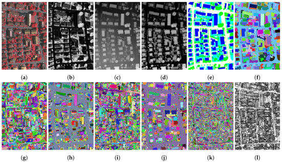
Figure 6.
Ilustration of ISPRS dataset (tile of Vaihingen): (a) False color orthophoto, (b) NDVI, (c) DSM, (d) nDSM, (e) reference map, (f) reference segmentation, (g,h) Felzenszwalb IRRG and nDSM, (i,j) Mean-shift IRRG and nDSM, (k) super-pixels, (l) confidence map. All segmentation and super-pixels maps are given in random pseudo-colors.
We conducted two additional experiments to compare the results provided by our method with the results of more traditional approaches. The first experiment was a post-classification fusion of four classification maps based on (1) Felzenszwalb segmentation of IRRG, (2) Felzenszwalb segmentation of nDSM, (3) mean-shift segmentation of IRRG and (4) mean-shift segmentation of nDSM. The fusion providing the final classification was based on a majority vote. The second approach was a before-segmentation fusion (i.e., a stack of IRRG+nDSM images). A first classification map was generated from this source after a mean-shift segmentation. A second classification map was derived from a Felzenszwalb segmentation. In all cases, the classifications were based on the random forest algorithm.
4.2. Results and Discussion
4.2.1. Partial Segmentation
In the first of the two additional experiments, we aim to evaluate the quality of the partial segmentations obtained with different thresholds (from to by step of ). We thus measure the quality of the retained super-pixels in terms of classification accuracy considering the F1 score. Figure 7 shows the F1 score vs the confidence value threshold plot per class. It shows that setting a high threshold for the confidence value yields fewer super-pixels but higher accuracy, which was expected. Nevertheless, we can also see that in some cases, the high-confidence super-pixels are incorrectly classified, thus leading to a lower overall score. However, it should be noted that such effects are observed with a small number of super-pixels, and consequently F1 score statistics are less significant.
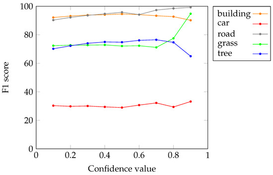
Figure 7.
Accuracy of the super-pixels (F1 score; y-axis) in each class according to the confidence value threshold (x-axis).
4.2.2. Full Segmentation
In the second experiment, we consider full segmentation. We previously discussed several strategies to build a full segmentation from a partial one. In order to draw generic conclusions from our experimental study, here we decided to keep all super-pixels (and their associated confidence map). First, using the previously described setup, we compare an object-based classification and a pixel-wise classification. Figure 8 illustrates the relevance of the GEOBIA paradigm, with—for instance—less salt and pepper noise in the classification map and more accurate borders in our method (Figure 8b) than when pixel values are used directly (Figure 8a).
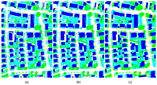
Figure 8.
(a) Pixelwise Classification, (b) Super-pixelwise classification, (c) Reference map. The color legend for the classes is as follows: building (blue), low vegetation (cyan), tree (green), impervious surface (white), car (yellow).
Furthermore, considering all super-pixels in the accuracy assessment avoids possible artifacts due to lack of statistical significance, as observed in the previous section. We thus introduce a novel evaluation protocol that modifies the computation of the underlying confusion matrix in order to weight each individual contribution of an element by its confidence level. Table 1 and Table 2 list the unweighted (original) and weighted (proposed) confusion matrices, where the unit is the number of pixels (but a similar conclusion can be drawn using the number of super-pixels). The values between those matrices cannot be compared directly due to the weighting by the confidence value, which lowers the values in Table 2 w.r.t. Table 1.

Table 1.
Unweighted confusion matrix.
Table 2.
Weighted confusion matrix.
To compare the matrices, we compute F1 scores for each class in both cases, and provide a comparison in Table 3. The systematic improvement of the weighted version over the unweighted one is clear. The car class is the only class for which there is no improvement in the F1 score, and this is probably due to the fact that the objects are small and difficult to classify. The F1 score of all the other classes is higher when accounting for the confidence level, i.e., the super-pixels resulting from a consensus are more likely to be well-classified than others. This supports our final proposal of using the super-pixels with their confidence level in a fuzzy classification framework.
Table 3.
F1 score of each class and average calculated from the original (unweighted) and proposed (weighted) confusion matrices.
4.3. Comparison with Other Fusion Strategies
In this paper, we chose to focus on fusion at the object level. When several data sources are available, it is also possible to conduct fusion at the pixel level (i.e., before segmentation) or at the decision level (i.e., after classification). We compare our approach with these two strategies, following the same classification scheme based on random forest.
Figure 9 illustrates the classification maps produced with the different strategies. In the case of post-classification fusion, we combine four maps (obtained with all combinations of two segmentation methods applied on two data sources) through a majority voting procedure (see Figure 9a). In contrast, Figure 9b,c show the use of Felzenszwalb and mean-shift segmentation methods respectively, when applied to a stack made of the two available sources, namely IRRG and nDSM data (pre-classification fusion). Visual comparison with our method (see Figure 8b), enables us to make several remarks.
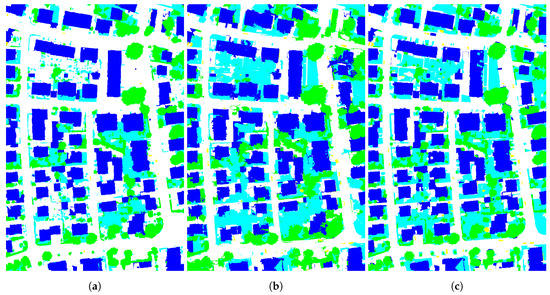
Figure 9.
(a) Post-classification fusion of four individual classifications derived from Felzenszwalb and mean shift segmentations on IRRG and nDSM respectively, (b) classified Felzenszwalb segmentation based on a before segmentation fusion of IRRG+nDSM, (c) classified mean shift segmentation based on a before segmentation fusion of IRRG+nDSM. The colors used for the classes are as follows: building (blue), low vegetation (cyan), tree (green), impervious surface (white), car (yellow).
The post-classification fusion greatly underestimates two out of the five classes (low vegetation and cars are often incorrectly classified as impervious surface). By stacking IRRG and nDSM into a single data source, pre-classification fusion leads to irregularly shaped object with the Felzenszwalb method. The results are more accurate with mean shift, emphasizing the sensitivity of the classification results to the segmentation method used (recall that as segmentation is an ill-posed problem, we cannotfind a perfect universal segmentation method). The results are somewhat similar to our method, showing that the combination process is able to rely on the most relevant segmentation map (or, by extension, the most relevant data sources) among those available.
These visual results are completed by quantitative evaluation (Table 4, Table 5, Table 6 and Table 7). The first one (Table 4) shows the F1 scores obtained for each class and averages obtained with the different segmentation strategies. Our method obtained the highest average F1-score, as well as the best results for the road and cars classes. The following tables provide deeper insights with confusion matrices measured between the different classes for each individual strategy. We can see the misclassification between grass and roads or cars and roads, as already shown visually.
Table 4.
F1 score of each class and average calculated using our proposed method and other fusion strategies (post- and before-segmentation, see Figure 9).
Table 5.
Confusion matrix obtained for post-classification fusion (Figure 9a).
Table 6.
Confusion matrix obtained for classified Felzenszwalb segmentation based on a before- segmentation fusion (Figure 9b).
Table 7.
Confusion matrix obtained for classified mean-shift segmentation based on a before-segmentation fusion (Figure 9c).
5. Conclusions
In the present paper, we deal with the combination of segmentations for which we propose a generic framework. This is a very topical issue, with numerous works in image processing, computer vision, as well as remote sensing. In the context of GEOBIA, segmentation is a critical element and there is no universal and optimal segmentation method able to deal with the different situations (multiple sensors, multiple dates, multiple spatial resolutions, etc.). Our framework builds upon previous work in relying on the super-pixels produced by intersecting input segmentations. However in contrast to existing methods, we do not rely on the original data but only on the segmentation maps, thus making it possible to use heterogeneous data sources. Furthermore, we propose a way to embed prior knowledge through a local or global weighting scheme. We define a new confidence score in each super-pixel that measures the local consensus between the different input segmentations and allows for possible multiple scales between them. We have demonstrated the relevance of this confidence score and illustrated how it can be used in different experimental setups, based on a publicly available dataset.
While these experiments provide initial insights into the proposed confidence measure, we still need to compare our framework with existing solutions for segmentation fusion. Nevertheless, let us recall that unlike existing methods, our framework is generic in the sense that it does not assume a single data source from which multiple segmentations are derived. Our confidence measure is based on a single criterion (revised local refinement error). Recently, some attempts have been made in segmentation fusion using multiple criteria [33], that are worth monitoring. Finally, the proposed weighting scheme relies on manual settings (based on the user’s prior knowledge). We believe the method will gain in robustness if those weights could be computed automatically (e.g., through machine learning).
Author Contributions
Conceptualization, Sébastien Lefèvre, David Sheeren and Onur Tasar; Data curation, Onur Tasar; Formal analysis, Onur Tasar; Investigation, Onur Tasar; Methodology, Sébastien Lefèvre, David Sheeren and Onur Tasar; Project administration, Sébastien Lefèvre; Software, Onur Tasar; Supervision, Sébastien Lefèvre and David Sheeren; Validation, Onur Tasar; Visualization, Onur Tasar; Writing—original draft, Sébastien Lefèvre and Onur Tasar; Writing—review & editing, Sébastien Lefèvre and David Sheeren.
Funding
This research was funded by the French Agence Nationale de la Recherche (ANR) under reference ANR-13-JS02-0005-01 (Asterix project).
Acknowledgments
The Vaihingen dataset was provided by the German Society for Photogrammetry, Remote Sensing and Geoinformation (DGPF) [29]: http://www.ifp.uni-stuttgart.de/dgpf/DKEP-Allg.html. The authors thank the anonymous reviewers for helping us to improve our paper.
Conflicts of Interest
The authors declare no conflict of interest.
References
- Hay, G.J.; Castilla, G. Geographic Object-Based Image Analysis (GEOBIA): A new name for a new discipline. In Object-Based Image Analysis: Spatial Concepts for Knowledge-Driven Remote Sensing Applications; Blaschke, T., Lang, S., Hay, G.J., Eds.; Springer: Berlin/Heidelberg, Germany, 2008; pp. 75–89. [Google Scholar]
- Blaschke, T. Object based image analysis for remote sensing. ISPRS J. Photogramm. Remote Sens. 2010, 65, 2–16. [Google Scholar] [CrossRef]
- Blaschke, T.; Hay, G.J.; Kelly, M.; Lang, S.; Hofmann, P.; Addink, E.; Feitosa, R.Q.; van der Meer, F.; van der Werff, H.; van Coillie, F.; et al. Geographic Object-Based Image Analysis—Towards a new paradigm. ISPRS J. Photogramm. Remote Sens. 2014, 87, 180–191. [Google Scholar] [CrossRef] [PubMed]
- Baatz, M.; Schape, A. Multiresolution segmentation: an optimization approach for high quality multi-scale image segmentation. In Angewandte Geographische Informations-Verarbeitung XII; Strobl, J., Blaschke, T., Griesebner, G., Eds.; Wichmann Verlag: Heidelberg, Germany, 2000; pp. 12–23. [Google Scholar]
- Cheng, H.; Jiang, X.; Sun, Y.; Wang, J. Color image segmentation: Advances and prospects. Pattern Recognit. 2001, 34, 2259–2281. [Google Scholar] [CrossRef]
- Dragut, L.; Csillik, O.; Eisank, C.; Tiede, D. Automated parameterisation for multi-scale image segmentation on multiple layers. ISPRS J. Photogramm. Remote Sens. 2014, 88, 119–127. [Google Scholar] [CrossRef]
- Ming, D.; Li, J.; Wang, J.; Zhang, M. Scale parameter selection by spatial statistics for GeOBIA: Using mean-shift based multi-scale segmentation as an example. ISPRS J. Photogramm. Remote Sens. 2015, 106, 28–41. [Google Scholar] [CrossRef]
- Johnson, B.; Xie, Z. Unsupervised image segmentation evaluation and refinement using a multi-scale approach. ISPRS J. Photogramm. Remote Sens. 2011, 66, 473–483. [Google Scholar] [CrossRef]
- Johnson, B.A.; Bragais, M.; Endo, I.; Magcale-Macandog, D.B.; Macandog, P.B.M. Image Segmentation Parameter Optimization Considering Within- and Between-Segment Heterogeneity at Multiple Scale Levels: Test Case for Mapping Residential Areas Using Landsat Imagery. ISPRS Int. J. Geo-Inf. 2015, 4, 2292–2305. [Google Scholar] [CrossRef]
- Bock, S.; Immitzer, M.; Atzberger, C. On the Objectivity of the Objective Function—Problems with Unsupervised Segmentation Evaluation Based on Global Score and a Possible Remedy. Remote Sens. 2017, 9, 769. [Google Scholar] [CrossRef]
- Zhang, J. Multi-source remote sensing data fusion: status and trends. Int. J. Image Data Fusion 2010, 1, 5–24. [Google Scholar] [CrossRef]
- Dalla-Mura, M.; Prasad, S.; Pacifici, F.; Gamba, P.; Chanussot, J.; Benediktsson, J.A. Challenges and Opportunities of Multimodality and Data Fusion in Remote Sensing. Proc. IEEE 2015, 103, 1585–1601. [Google Scholar] [CrossRef]
- Gomez-Chova, L.; Tuia, D.; Moser, G.; Camps-Valls, G. Multimodal Classification of Remote Sensing Images: A Review and Future Directions. Proc. IEEE 2015, 103, 1560–1584. [Google Scholar] [CrossRef]
- Cho, K.; Meer, P. Image segmentation from consensus information. Comput. Vis. Image Underst. 1997, 68, 72–89. [Google Scholar] [CrossRef]
- Mahmoudi, F.T.; Samadzadegan, F.; Reinartz, P. A Decision Level Fusion Method for Object Recognition Using Multi-Angular Imagery. ISPRS Int. Arch. Photogramm. Remote Sens. Spat. Inf. Sci. 2013. [Google Scholar] [CrossRef]
- Franek, L.; Abdala, D.; Vega-Pons, S.; Jiang, X. Image Segmentation Fusion using General Ensemble Clustering Methods; ACCV: Queenstown, New Zealand, 2010. [Google Scholar]
- Khelifi, L.; Mignotte, M. A Novel Fusion Approach Based on the Global Consistency Criterion to Fusing Multiple Segmentations. IEEE Trans. Syst. Man Cybern. Syst. 2017, 47, 2489–2502. [Google Scholar] [CrossRef]
- Li, Z.; Wu, X.; Chang, S. Segmentation Using Superpixels: A Bipartite Graph Partitioning Approach; CVPR: Providence, RI, USA, 2012. [Google Scholar]
- Karadag, O.; Senaras, C.; Vural, F. Segmentation Fusion for Building Detection Using Domain-Specific Information. IEEE J. Sel. Top. Appl. Earth Obs. Remote Sens. 2015, 8, 3305–3315. [Google Scholar] [CrossRef]
- Ozay, M.; Vural, F.; Kulkarni, S.; Poor, H. Fusion of Image Segmentation Algorithms Using Consensus Clustering; ICIP: Melbourne, Australia, 2013. [Google Scholar]
- Ozay, M. Semi-Supervised Segmentation Fusion of Multi-Spectral and Aerial Images; ICPR: Stockholm, Sweden, 2014. [Google Scholar]
- Vitaladevuni, S.; Basri, R. Co-Clustering of Image Segments Using Convex Optimization Applied to EM Neuronal Reconstruction; CVPR: San Francisco, CA, USA, 2010. [Google Scholar]
- Vicente, S.; Kolmogorov, V.; Rother, C. Cosegmentation Revisited: Models and Optimization; ECCV: Heraklion, Crete, 2010. [Google Scholar]
- Dong, X.; Shen, J.; Shao, L.; Yang, M. Interactive cosegmentation using global and local energy optimization. IEEE Trans. Image Process. 2015, 24, 3966–3977. [Google Scholar] [CrossRef] [PubMed]
- Randrianasoa, J.; Kurtz, C.; Desjardin, E.; Passat, N. Binary Partition Tree construction from multiple features for image segmentation. Pattern Recognit. 2018, 84, 237–250. [Google Scholar] [CrossRef]
- Martin, D. An Empirical Approach to Grouping and Segmentation. Ph.D. Thesis, University of California, Berkeley, CA, USA, 2002. [Google Scholar]
- Saaty, T.L. A scaling method for priorities in hierarchical structures. J. Math. Psychol. 1977, 15, 234–281. [Google Scholar] [CrossRef]
- Weber, J.; Lefèvre, S. Fast quasi-flat zones filtering using area threshold and region merging. J. Vis. Commun. Image Represent. 2013, 24, 397–409. [Google Scholar] [CrossRef]
- Cramer, M. The DGPF test on digital aerial camera evaluation – overview and test design. Photogramm. Fernerkund. Geoinf. 2010, 2, 73–82. [Google Scholar] [CrossRef] [PubMed]
- Zhang, K.; Chen, S.C.; Whitman, D.; Shyu, M.L.; Yan, J.; Zhang, C. A progressive morphological filter for removing nonground measurements from airborne LIDAR data. IEEE Trans. Geosci. Remote Sens. 2003, 41, 872–882. [Google Scholar] [CrossRef]
- Felzenszwalb, P.F.; Huttenlocher, D.P. Efficient graph-based image segmentation. Int. J. Comput.Vis. 2004, 59, 167–181. [Google Scholar] [CrossRef]
- Comaniciu, D.; Meer, P. Mean shift: A robust approach toward feature space analysis. IEEE Trans. Pattern Anal. Mach. Intell. 2002, 24, 603–619. [Google Scholar] [CrossRef]
- Khelifi, L.; Mignotte, M. A Multi-Objective Decision Making Approach for Solving the Image Segmentation Fusion Problem. IEEE Trans. Image Process. 2017, 26, 3831–3845. [Google Scholar] [CrossRef] [PubMed]


© 2019 by the authors. Licensee MDPI, Basel, Switzerland. This article is an open access article distributed under the terms and conditions of the Creative Commons Attribution (CC BY) license (http://creativecommons.org/licenses/by/4.0/).