Integrated Multiscale Method for Obtaining Accurate Forest Surface Area Statistics over Large Areas

Abstract

Forest surface area is a fundamental input for forest-related research, such as carbon balance, biodiversity conservation, and ecosystem functioning and services. However, an accurate assessment of the area of forestland in China is not available because the forested area is usually calculated as a 2D projected area rather than a 3D surface area, and the impact of changes in the surface terrain on the area is ignored. In this study, we propose an integrated multiscale method that combines geomorphic regionalization and surface area algorithms to calculate the forest surface area in China. The results show that (1) China’s forested area is approximately 4.91% larger than the conventional estimates and corresponds to a carbon storage estimate that is approximately 383.72 million tons higher; (2) the integrated multiscale method exhibits good adaptability and high precision for large-scale surface area calculations; and (3) the calculation results of this method are superior to those of remote sensing data or single surface area algorithms, and the calculation efficiency is high.

1. Introduction

As an important part of the Earth’s biosphere, forests are a key factor in maintaining the global ecological balance by serving as carbon sources and sinks and removing carbon dioxide (CO₂) through Biomass Energy with Carbon Capture and Storage (BECCS) [1,2,3]. Moreover, forests also provide material resources for human survival and development and ecosystem services for local people. According to the current land use classification of China [4,5], forestland refers to land covered with trees, bamboo, shrubs, and coastal mangrove forests. Spatial changes in forestland, such as an increase or decrease in area and the replacement of types, can have great impacts on ecology and human society [6]. Therefore, accurate forestland resource statistics have great realistic and strategic significance [3].

Forest resource inventories are traditionally conducted via ground surveys at a high level of detail for relatively small areas. The advantage of this method is that the field data are detailed and accurate [7]. However, the long field survey time means that information is slow to be updated and thus may not reflect the rapid changes caused by development. Additionally, the inconsistent timing of field surveys in different regions of China affects the comparability of data. Therefore, researchers have introduced remote sensing data into forestland statistics due to their high spatial-temporal resolution; however, remote sensing techniques yield the projected area (two-dimensional area, 2D area) instead of the real undulating surface area (three-dimensional area, 3D area), which is an important basic indicator of forestland area [8,9,10,11,12]. Forestland is mainly present in areas with complex topography and large topographic relief in China. Consequently, calculations without height data will cause large bias in subsequent research, such as biomass and carbon sinks [12,13,14,15,16,17]. To solve this problem, it is a feasible way to accurately estimate forestland surface area by overlaying remote sensing and digital elevation model (DEM) data and using algorithms to simulate the area of elements along the surface of the earth based on the actual relief amplitude [17,18,19].

Researchers have performed a number of important studies regrading this problem. Some studies have calculated the surface area by combining the slope secant with grid data, which uses each grid of the remote sensing data as a calculation unit, and calculating the secant of the angle of this inclined unit; the surface area of this unit is the product of its secant and its projected area, and the total surface area is the sum of each unit’s surface area [12,20,21,22,23,24]. Additionally, differential methods based on numerical integration are used to approximate the surface. This approximation is generally achieved by constructing the area microelements, which are generally determined by the four vertex positions and the polygonal relationship of the grid data. In this process, the position relationship between the polygon boundary and the grid is frequently determined. There are many decision loops in the determination algorithm that affect the efficiency of the surface area calculation [25,26]. Other scholars have used the relationship between the surface area and ellipsoids to study the surface fitting method [27,28,29,30,31], which mainly employs triangular fitting, using spatial triangulation to fit the topographic relief [1,32,33,34,35]. According to the different methods of dealing with discrete points, triangulation algorithms can be classified into three categories: a growth algorithm that is easy to implement but inefficient [36,37,38,39]; a divide-and-conquer algorithm that has the highest efficiency but frequently calls recursively; and a point-by-point insertion algorithm with a simple process and a small memory requirement [35,40,41,42,43,44,45,46,47]. In addition, most of these studies focus on a single method, and no cross comparison of the advantages and disadvantages of these methods or discussion of the scope of their applications is available. Many studies are concentrated on small ranges, which have limited data and low accuracy [12,19,24,25]. Furthermore, surface area calculation often requires massive computation. When the region of interest is expanded, the surface structure becomes more complex; topographic factors, such as the slope and undulation, change more dramatically; and the data volume increases geometrically. For large-scale applications, the calculation accuracy and efficiency of existing studies cannot handle the complex situations presented by high-precision data with large volumes and cannot meet the application needs.

In this study, we attempted to solve these problems based on the above studies. Considering the complex terrain environment, forest fragmentation distribution characteristics, and objective realities of large amounts of data, we overlay DEM data with remote sensing data, use the mean change point and system clustering analysis methods to partition the national-scale region, identify suitable surface area algorithms for every type of geomorphic area, define geomorphic dominance and combine it with a surface area calculation algorithm, and select the appropriate combination for every region. Highly efficient, accurate statistics for forestland areas are obtained, thus providing a theoretical basis for more reasonable carbon emission statistics and climate change research.

2. Materials and Methods

2.1. Data Sources

Three types of data are used in this study: Shuttle Radar Topography Mission (SRTM) data, remote sensing interpretation data (Chinese GlobeLand30), and national basic geographic information.

Shuttle Radar Topography Mission data are available from the United States Geological Survey (USGS) website (https://earthexplorer.usgs.gov/), which is an international research effort that provides land elevation data for over 80% of the globe. The effort was conducted by the US National Aeronautics and Space Administration (NASA) and the US National Geospatial-Intelligence Agency (NGA). The SRTM 1 Arc-Second Global used in this study provides high-precision terrain grid data with voids filled. Its horizontal datum is WGS84, vertical datum is EGM96, and spatial resolution is 1 arc-second (approximately 30 m) [36].

The Chinese GlobalLand30 datasets are high-resolution maps of the Earth’s land cover, including forests and nine other types [37]. The data were extracted from multispectral images with a resolution of 30 m, including the US Earth-observing Landsat satellite sensors, Landsat 5 Thematic Mapper (TM), and Landsat 7 Enhanced Thematic Mapper Plus (ETM+) [38], China’s Environmental Disaster Alleviation Satellite (HJ-1), and a large amount of auxiliary data. GlobalLand30 used a hierarchic method for image classification; the classification scheme of forest is land with greater than 30% vegetation cover, including deciduous and coniferous forests and sparse woodland with 10–30% cover. Its reference ellipsoid is the WGS84 ellipsoid, and the data adopt the UTM projection, the WGS84 coordinate system, and 6-degree zoning. A rule-based workflow and multisource integration were conducted before publication to ensure the quality and consistency of the data. The comprehensive accuracy of the forest data was 89% [38].

The national basic geographic information data were obtained from the National Geomatics Center of China (NGCC), which is a government agency that fulfills missions to construct, manage, and distribute national fundamental geo-information data and archives, including national borders, provincial boundaries, and major highways.

2.2. Research Concepts and Technical Routes

We established an integrated multiscale method of calculating forestland area via the optimum combination of geomorphic regionalization and surface area calculation methods; thus, the forestland area of China was calculated. The technical route is shown in Figure 1.

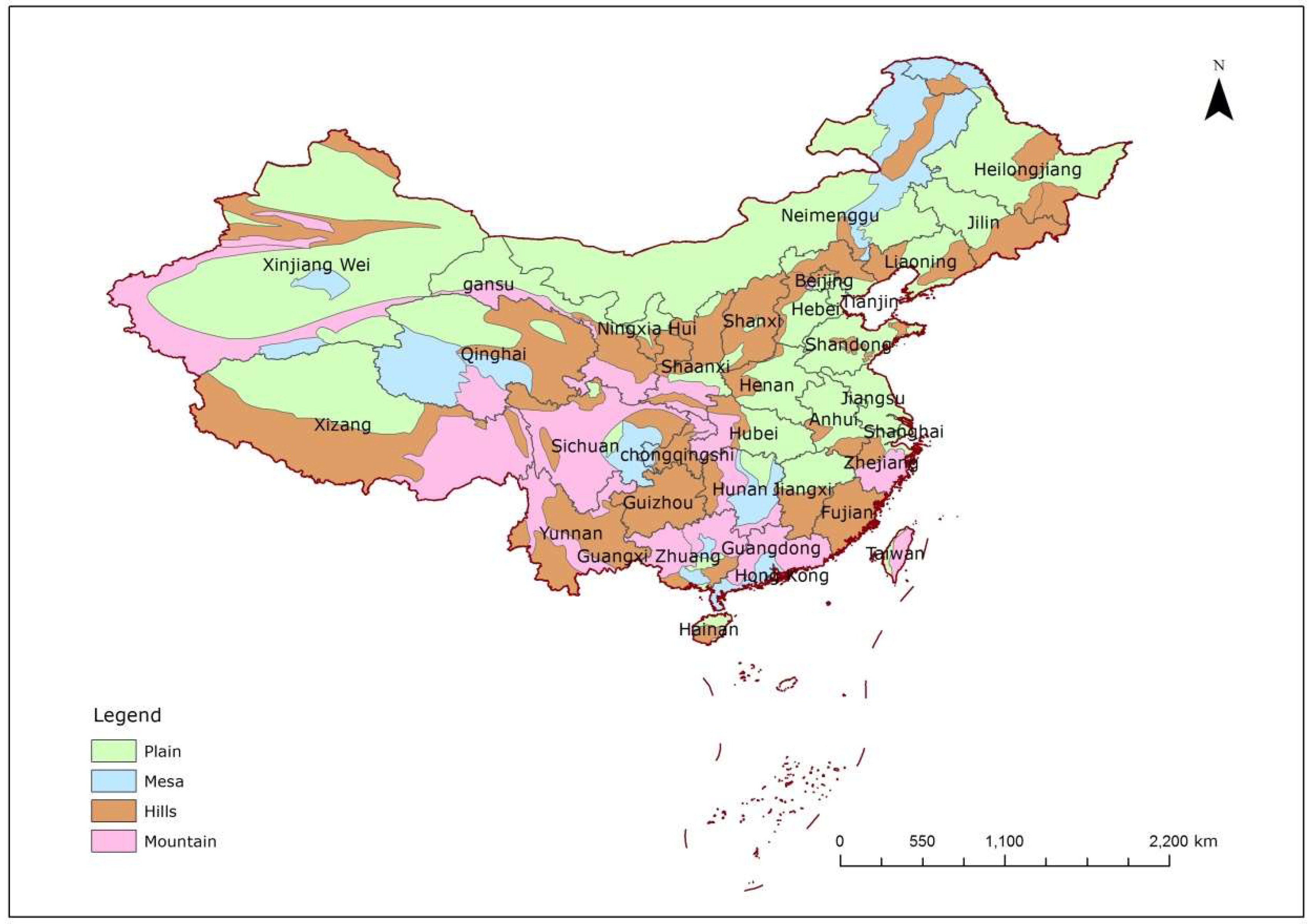
2.3. Geomorphic Regionalization

Geomorphic regionalization divides a region into different sub-regions according to the similarities and differences of the geomorphic areas based on the principles of relative consistency and geomorphic integrity. Geomorphic aspects mainly include elevation, relief amplitude, etc. The relief amplitude is an important index for quantitatively describing the geomorphology and for classifying geomorphic types [39,40]. This parameter represents the height difference between the highest and lowest points in a certain area. Therefore, relief amplitude is the most relevant to this study, and we selected it as the index for division and used the system clustering analysis method, which combined bottom-up clustering and top-down division (Figure 2), to determine every geomorphic area and the associated boundaries and achieve geomorphic regionalization of large areas.

2.3.1. Relief Amplitude Algorithm

“Determined area” is the optimal statistical unit of relief amplitude. The study shows that the topographic relief changes with the area in a logarithmic curve [41,42], and thus the optimal statistical unit is the curve mutation point at which the curve changes from steep to shallow. For this purpose, we introduce the statistical mean change point analysis method by increasing the window used to calculate the relief to obtain that point. The calculation process is as follows:

With sample sequence H₀, perform the following task:

• Set i = 2 ... n; for each i, the sample is divided into two sections: X₁, X₂ ... X_i-1 and X_i, X_i+1 ... X_n. Calculate the arithmetic mean and statistic Si for each sample.

  $$S_i={\displaystyle \sum }_{t=1}^{i-1}{(X_t-\overline{X_{i1}})}^2+{\displaystyle \sum }_{t=1}^N{(X_t-\overline{X_{i2}})}^2$$

  (1)
• Compute statistic S for the original sample.

  $$\overline{X}={\displaystyle \sum }_{t=1}^N{X}_t/N$$

  (2)

  $$S={\displaystyle \sum }_{t=i}^N{(X_t-\overline{X})}^2$$

  (3)
• Calculate the expectation.

  $$\mathrm{E}\left(S-S_i\right),i=2,3,···,N$$

  (4)
• The greatest difference between S and S_i is the change point, which is the optimal statistical unit in this study.

Then, DEM data are traversed in the optimal statistical unit to obtain relief amplitude data.

2.3.2. System Clustering Division Method

Considering that regionalization takes into account the overall topography and the distribution continuity simultaneously, "top-down" division and "bottom-up" clustering are commonly used in research. The former operates from the whole region to the unit, and the latter operates from the unit to the whole region [43]. According to the characteristics of area measurement and the precision evaluation requirement, we use the two methods in coordination as follows: first, the region is divided from top to bottom based on the provincial administrative boundaries; and second, the basic geomorphic units in every region are clustered with the iterative clustering algorithm. To ensure geomorphic integrity, the clustering results are manually adjusted, and the boundaries are checked to ensure that each region is a convex polygon and the boundary is complete without broken line segments.

We quantified the classification standard of geomorphic type according to the digital landform mapping specification. It is divided into seven levels according to the terrain undulation: plain (<30 m), mesa (30~70 m), hills (70~200 m), low relief amplitude mountain (LRAM) (200~500 m), medial amplitude mountain (MAM) (500~1000 m), high amplitude mountain (HAM) (1000~2500 m), and higher amplitude mountain (HerAM) (>2500 m). The code (GeoID) ranges from 1–7. At the same time, the geomorphic dominance (GeoDominance) is defined for subsequent area calculation. The region’s GeoDominance of a certain geomorphology is the area proportion of that geomorphology in the region. The area proportion is calculated by the projected area to avoid the impact of relief amplitude, and the formula is as follows:

$$\mathrm{GeoDominance}=\frac{{\mathrm{region}}^{\prime }\mathrm{s}\mathrm{projected}\mathrm{area}\mathrm{of}\mathrm{certain}\mathrm{geomorphic}}{{\mathrm{region}}^{\prime }\mathrm{s}\mathrm{projected}\mathrm{area}}\times 100\%,$$

(5)

2.4. Surface Area Calculation Algorithm

2.4.1. Slope-Based Calculation Algorithm

This algorithm calculates the surface area by using each grid as a calculation unit and treats it as an inclined surface to calculate the surface area from its slope. The relationship between the surface area and the projection area is as follows:

$$S_1=\frac{S_2}{\cos \mathrm{A}}=S_2\times \sec \mathrm{A},$$

(6)

where S₁ is the surface area, S₂ is the projected area, A is the angle of the slope, and cosA and secA are the cosine and secant of A, respectively. The following formula is used to calculate the secant value of the slope (A) in Equation (6).

$$\sec \mathrm{A}=1/\cos \frac{A\times 3.1415926}{180},$$

(7)

Using the window differential analysis method to traverse the DEM [24], the slope (A) of the window center point is calculated as follows:

$$\mathrm{slope}=\arctan \sqrt{{(\frac{\left(e_8+2e_1+e_5\right)-\left(e_7+2e_3+e_6\right)}{8\times cellsize})}^2+{(\frac{\left(e_7+2e_4+e_8\right)-\left(e_6+2e_2+e_5\right)}{8\times cellsize})}^2},$$

(8)

The two squared values are the slopes in the x- and y-directions, respectively. If the center point has no data, the slope value of this grid should be set as null. Any adjacent point with no data will be assigned the value of the central point.

The projected area obtained from the raster data and the computed secant values are substituted into Equation (6) to obtain the surface area.

2.4.2. Triangular Irregular Network (TIN)-Based Calculation Algorithm

The TIN algorithm uses spatial triangulation to fit the undulating ground surface and achieves a three-dimensional visualization of the surface details. The sum of the triangle area can be approximately regarded as the surface area [44]. Considering the massive amount of data in this study, we improve the point-by-point insertion algorithm by instituting a directional search and locating the insertion points based on topological relationships followed by a check of the elevation of the insertion points. If two triangles have the same elevation value, they are considered to be in the same plain and are merged into one triangle.

After the triangular network is completed, the surface area is the sum of the triangle areas in the network [45]. The area of each triangle is obtained by Heron′s formula (Formula (9)).

$$S=\sqrt{p\left(p-a\right)\left(p-b\right)\left(p-c\right)},$$

(9)

where variables a, b, c are the three sides of the triangle and calculated by the vertex elevation, and p is half of the triangle’s circumference. A triangular network has a strong graphic structure and can fit well in regions with undulating terrain.

2.4.3. Simpson-Based Calculation Algorithm

This method assumes that the surface is composed of several smooth curved surfaces and uses the projection area and integral surface to calculate the surface area (Figure 3).

By referring to the calculation method of the polygon ellipsoid area, we modify the original two-dimensional composite Simpson formula (Formula (10)) to three dimensions by two-layer approximation.

$$S={{\displaystyle \int }}_a^{b}f\left(x\right)dx=\frac{b-a}{6}\left[f\left(a\right)+f\left(\frac{a+b}{2}\right)f\left(b\right)\right],$$

(10)

(1) The first layer: approximation of the length of the curve:

Let f(x) be a secant value representing the angle between the vector in the upward direction of the x-point and the unit vector in the positive direction of the x-axis.

The length of the curve is determined as follows:

$$\mathrm{F}\left(\mathrm{x}\right)= {{\displaystyle \int }}_{x_0}^{x_n}f\left(x\right)dx$$

(11)

From Simpson′s formula, the following equation can be deduced:

$$\underset{x_0}{\overset{x_2}{{\displaystyle \int }}}f\left(x\right)dx= \frac{x_1-x_0}{6}\left(f\left(x_0\right)+4f\left(x_1\right)+f\left(x_2\right)\right)$$

(12)

$$\begin{array}{cc}\hfill \mathrm{F}\left(\mathrm{x}\right)& =\frac{1}{2}(\frac{width}{6}\left(f\left(x_0\right)+4f\left(x_1\right)+f\left(x_2\right)\right)+\frac{width}{6}\left(f\left(x_1\right)+4f\left(x_2\right)+f\left(x_3\right)\right)+\dots \hfill \\ & +\frac{width}{6}\left(f\left(x_{n-2}\right)+4f\left(x_{n-1}\right)+f\left(x_n\right)\right))\hfill \end{array}$$

(13)

Parameter F(x) is determined as follows:

$$\mathrm{F}\left(\mathrm{x}\right)= \frac{width}{12}\left(f\left(x_0\right)+f\left(x_n\right)+5{\displaystyle \sum }_{i=1}^{n-1}f\left(x_i\right)\right)$$

(14)

where

$$\mathrm{f}\left(x_i\right)=\{\begin{array}{c}\sqrt{{\left(h\left(x_1\right)-h\left(x_0\right)\right)}^2+widt{h}^2}, x=0\\ \sqrt{{\left(h\left(x_i\right)-h\left(x_{i-1}\right)\right)}^2+widt{h}^2}, x>0 \end{array}$$

(15)

h(x_i) is the elevation value at the x_i point, and width is the width in the x-direction.

(2) The second layer: approximation of the area:

The result of the previous step is that F(y) is a function representing the length of the curve at the y point.

The surface area can be expressed as follows:

$$\mathrm{G}\left(y\right)= {{\displaystyle \int }}_{y_0}^{y_n}F\left(y\right)dy$$

(16)

Similar to the length approximation derivation process, the following equation can be deduced:

$$\mathrm{G}\left(x\right)= \frac{height}{12}\left(F\left(y_0\right)+F\left(y_m\right)+5{\displaystyle \sum }_{j=1}^{m-1}F\left(y_j\right)\right)$$

(17)

where height is the width in the y-direction of the grid.

2.5. Integrated Multiscale Method for the Surface Area Calculation

First, the above surface area algorithms are implemented in one program using the language Python; second, they are applied to typical regions of all geomorphic types and an error analysis is carried out on the calculated results to obtain the optimal combination of surface area algorithms suitable for each geomorphic type.

After the above preparations, a kit method that divides the study area into geomorphic regions is used to calculate the surface area by calling the corresponding surface area algorithms according to the region’s geomorphic types. The results are weighted by the dominance of each geomorphic type. The sum of each region’s area is the surface area of the study area.

3. Data Processing

3.1. Appropriate Surface Area Algorithm Selection

The core of this study is the identification of suitable surface area algorithms for different geomorphic types. For this reason, we selected 210 areas from the typical distribution areas of seven geomorphic types as test areas and 30 areas for each geomorphic type, and the projected area of each test area was approximately 1000 km². The surface area calculation of each test area was carried out using the three methods presented in Section 2.4. The suitable surface area algorithms were obtained through comparison. The location of each test area is shown in Figure 4.

For each test area, a DEM with a resolution of 5 m was generated with contour lines, and the contour interval was 5 m. For the 5 m and 30 m DEMs, all three surface area algorithms were used in the calculations, and the average value of the 5 m DEM was taken as the reference value for the true surface area value. Then, these results were compared with the results from the 30 m DEM, and the absolute and relative errors were calculated. The best surface area algorithm was selected based on the relative error distribution of every geomorphology (

Table 1. Relative error number distribution.

GeoID	Simpson-Based Area		Sloped-Based Area		TIN-Based Area
	MinError	MinDifference	MinError	MinDifference	MinError	MinDifference
1	8	3	19	11	3	5
2	17	12	8	7	5	3
3	11	6	1	5	18	1
4	4	0	0	6	26	0
5	1	0	0	1	29	0
6	1	0	1	0	28	1
7	0	0	0	1	30	0

). MinError means that this algorithm had a minimum relative error among the three algorithms, and MinDifference means that the algorithm had a minimum difference with the algorithm of minimum relative error.

Generally, the algorithm with the smallest relative error (MinError) was selected. However, in some geomorphic areas, the relative error between two algorithms was similar (with a difference <0.5%), and their differences from other algorithms were large; thus, the mean values of these two algorithms were selected to reduce the random error caused by the samples.

The results show that the TIN-based algorithm performs better in areas with large relief and continuous changes, the Simpson-based algorithm is efficient and accurate in mesa areas, and the slope-based algorithm performs better than the first two methods in areas with gentle rolling topography and accurately depicts the topographic details in areas with small relief.

Based on the above conclusions, a suitable surface area algorithm was selected for the seven types of geomorphic areas (

Table 2. Surface area statistics.

GeoID	Geomorphology	Algorithm
1	Plain	Slope
2	Mesa	Simpson
3	Hills	$\overline{\mathrm{Simpson}+\mathrm{TIN}}$
4	Low relief amplitude mountain	TIN
5	Medial amplitude mountain	TIN
6	High amplitude mountain	TIN
7	Higher amplitude mountain	TIN

).

3.2. National Geomorphic Regionalization

By dividing the national area to obtain the distribution of geomorphic types, we can perform area calculations on the basis of the methods presented below, i.e., Section 3.1. For the convenience of subsequent comparative analysis with statistical data, the top-down division of the national DEM was first carried out according to provincial boundaries. The regions of Hong Kong and Macao are too small to include in the division. Then, the regions were traversed sequentially to calculate the average value of relief amplitude by increasing the rectangular window. The logarithm of the results was taken to establish the sample sequence X (X = {X_i, i = 1, 2, 3 ... 29}). The values of the statistics S and S_i of sample series X and the differences between them were calculated. The corresponding window at the maximum difference value was the optimal statistical unit to extract the terrain undulation. The DEM data of each province (excluding Hong Kong, Macao, and the sea area) were traversed at this unit to obtain the relief amplitude data. Using the above classification index to classify the relief degree, Iterative Self-Organizing (ISO) unsupervised clustering was conducted to obtain the national geomorphic distribution.

Based on the China Geomorphic Regionalization System [43], the clustering results were adjusted manually. The main principles are that the dominance degree of the main geomorphic types in the region should be greater than 50% and the area should not be less than 9000 km². Finally, 119 geomorphic sub-regions are obtained, and they are overlain on the national DEM and clipped to obtain the national geomorphic regions (excluding Hong Kong, Macao, and sea areas).

For the geomorphic attribution of each region (DivID), GeoDominance was taken as a criterion for judging, and the DivID was the geomorphic type with the highest value. The regionalization distribution is shown in Figure 5. The geomorphic type (GeoID) and GeoDominance information in the area were stored in the region’s attribute table for subsequent calculations.

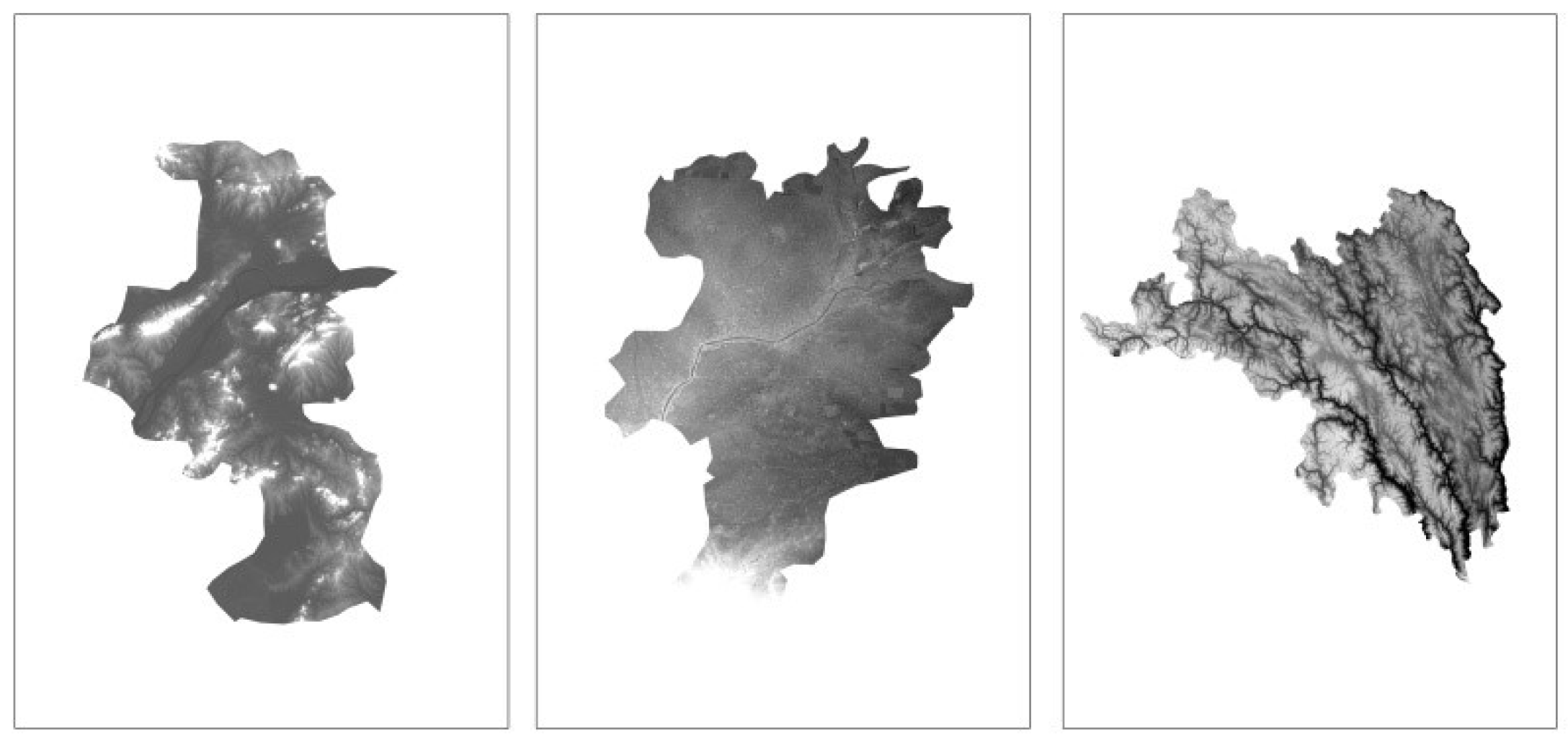
3.3. National Forestland DEM Acquisition

The data on forestland cover were extracted from GlobeLand30-2010 data [38]. The DEM data for China were clipped based on the forestland data to obtain the forestland DEM data for the whole country (Figure 6).

3.4. Forestland Surface Area Calculation

The arcpy package is imported into the aforementioned Python program to process the DEM data. Based on

Table 3. Calculation results for the surface area at different resolutions in the verification area.

Resolution Ratio of DEM (m)	Surface Area (km2)	Absolute Error (km2)	Relative Error (%)
5	5312.22	0	0
30	5287.82	24.4	0.46

, GeoID is used to call the area algorithm and to embed it in the Python program.

Since DivID ignores geomorphic areas with small proportions, such as MAM/HAM/HerAM, and because the area algorithms differ among different geomorphic types, we use multiple GeoIDs for each region to call the corresponding area surface algorithms and sum the calculation results weighted by the GeoDominance to reduce the error. The result of the summation is the national forestland surface area.

4. Results and Discussion

4.1. Accuracy Evaluation of the Surface Area Integrated Multiscale Method

A certain area in Western China was selected as the verification area; its elevation range is 1,354~5,931 m with a standard deviation of 792.14 m (Figure 7). The 5-m DEM was generated with 1:50,000 contour lines of this area, and the surface area calculation results were used as the reference value to evaluate the accuracy of the surface area calculation based on the SRTM DEM. The absolute and relative errors were 24.4 km² and 0.46%, respectively (Table 3). Therefore, the calculation method used for the surface area calculation in this paper has high accuracy.

4.2. Comparative Analysis with the Existing Literature

To verify that the surface area integrated multiscale method is superior to the traditional algorithm in terms of the area calculation accuracy, this paper referred to the example areas of Wang Xiuyun [24], Yuan Weiping [46], and Zeng Zhen [18] (Figure 8) and used the original method and the integrated multiscale method to calculate the surface areas of these regions. The original method used in the study of Xiuyun and Zeng Zhen was a slope-based algorithm based on the projected area and average secant of the slope of the whole region; Yuan Weiping used a Simpson-based method that cuts the grid data into strips in the x- and y-directions. The accuracy was evaluated with the method presented in Section 4.1. The area increment is the difference between the surface area and the projected area. The calculation results are shown in

Table 4. Comparison of surface area calculation methods between this study and the literature.

Region	Area Increment (%)		Relative Error (%)
	Original Paper	Integrated Multiscale Method	Original Paper	Integrated Multiscale Method
Forestland of Nanjing	0.016	0.40	0.56	0.16
Dongying	0.18	0.06	2.31	0.60
Changdu	12.68	15.98	12.78	1.97

.

The comparison in Table 4 shows that the integrated multiscale method for surface area has the lowest relative error and relatively high area increment in all three areas.

The integrated multiscale method reduces the error in many aspects to improve the calculation accuracy, such as the classification of the geomorphology to carry out targeted calculations for better simulations of surface relief and selection of appropriate algorithms for each geomorphology. The mean was used to reduce the error caused by the differences between the algorithms, and GeoDominance was defined to better adapt to the complex topography.

In terms of the area algorithm, the integrated multiscale method improves on previous research by performing a comprehensive comparison of seven geomorphic types with three algorithms, clarifies the characteristics and application scopes of the algorithms, defines GeoDominance, and uses it to combine the system clustering division method and three surface area calculation algorithms. As the relief amplitude changes, the appropriate surface area algorithm changes from slope-based to Simpson-based, and finally to TIN. The key of the TIN algorithm is the selection of the starting triangle and the improvement of the search path length. The Simpson-based method simplifies many judgments and loops in the previous process of building the area element via a two-layer approximation and improves the calculation efficiency while ensuring accuracy. GeoDominance can identify geomorphologies with small proportions in the area calculation, and for areas with mixed geomorphologies, it also ensures that the appropriate algorithms for every geomorphology are reflected in the calculation results.

Therefore, the integrated multiscale method provides higher precision than the single surface area calculation method under the same positioning coordinate precision.

4.3. Analysis of the Calculation Results for Forestland Surface Area in China

4.3.1. Calculation Results of Forestland Surface Area in China

The sum of the area of all the provinces (i.e., the national forestland surface area) is 2,280,202.76 km².

Table 5. Forestland surface area of each province.

Province	Forest Surface Area (km2)	Province	Forest Surface Area (km2)
Anhui	37,435.59	Jilin	75,717.79
Beijing	5454.40	Liaoning	52,001.74
Chongqing	30,603.30	Neimenggu	236,926.96
Fujian	81,755.81	Ningxia	5158.87
Gansu	47,743.13	Qinghai	33,971.97
Guangdong	89,843.17	Shaanxi	83,054.29
Guangxi	134,147.17	Shandong	25,914.02
Guizhou	59,436.40	Shanghai	600.04
Hainan	17,954.62	Shanxi	23,084.55
Hebei	42,763.13	Sichuan	185,620.51
Heilongjiang	193,203.10	Taiwan	23,751.50
Henan	33,873.06	Tianjin	961.28
Hubei	61,493.49	Xinjiang	68,766.10
Hunan	99,316.11	Xizang	155,723.22
Jiangsu	10,771.92	Yunnan	199,553.41
Jiangxi	100,903.04	Zhejiang	62,699.06

shows the forestland surface area for each province.

To perform a more comprehensive analysis of the national forestland surface area calculated by the integrated multiscale method and evaluate the underestimation of forestland area by traditional planar measurements and projected area substitution methods in the statistical process, the surface area was compared between the projected and statistical areas. The statistical data of each province’s forestland were obtained from the website of the Chinese National Bureau of Statistics and generally calculated by ground surveys, which means that the area data are 2D data.

4.3.2. Comparison with the Projected Area

For the calculation of the projected area, the number of grids in each region was first counted, and the projected area is the product of the grid number and the grid area. The sum of the projected areas of the regions is the projected area of national forestland, which is 2,160,470.47 km². The difference between the surface area and the projected area, as well as the area increment based on the projected area, were calculated (Figure 9), and the results can be treated as the area increment obtained by the surface area algorithm (Figure 10). The area increment ratio is the area increment percentage of the projected area, which suggests that the national forestland area has increased by 5.54% based on the projected area. Figure 6 shows the relationship between the average relief amplitude and the increment ratio of the projected area of each province. The provinces in the two charts are sorted by their average relief amplitudes.

Figure 9 shows that the 3D surface area of forests in each province is greater than the 2D projected area of forestland. The increment ratio of the projected area in Figure 10 is the area increment proportion of the projected area. Figure 10 shows that the area increment has a certain correlation with the average relief amplitude, although the change trend is not completely consistent with the average amplitude and is divided into the following four cases: (1) provinces with large average relief amplitude and concentrated geomorphic distribution of forestland, such as Xizang, Taiwan, and Sichuan, exhibit high area increment ratios consistent with large relief amplitude; (2) the average relief amplitude is large, but the geomorphic distribution of forestland is mixed, such as in Guangdong, Fujian, and Guizhou, and the area increment is not high relative to the larger undulations; (3) the average relief amplitude is small, but the geomorphic distribution of forestland is concentrated, such as in Xinjiang, whose unique geomorphology (i.e., two basins sandwiched among three mountains) results in a high area increment ratio; and (4) in provinces with a small average relief amplitude and decentralized distribution of forestland, such as Ningxia and Hainan, the topographic relief has less influence on the surface area calculation.

4.3.3. Comparison with Statistical Data

The remote sensing images used in this study were from 2010, and the forestland area of each province in 2010 was determined and compared with the surface area (Figure 11 and Figure 12). Compared with the statistical data, the percentage increase in forestland area measured in this paper reached 4.91%, representing a previous underestimation of 106,763.76 km². Based on the difference and increment ratios of the statistical area and the projected area (12,968.53 km² and 0.60%, respectively), most of the distribution of forestland used in the calculation of the projected area and the statistical area overlap, and the above number of 106,763.76 km² can be considered the underestimated area of forestland instead of a calculation error.

Provinces in the above charts are sorted by the average relief amplitude. As shown in the analysis in Figure 11 and Figure 12, the change in the statistical area is generally similar to that of the projected area. Some provinces, however, have changed, and we speculate there may be two reasons for the differences: (1) most forests in provinces, such as Henan, are distributed in the plains and low relief amplitudes are correlated with small area increment; (2) urban provinces, such as Shanghai and Jiangsu, along with mainly desert provinces, such as Neimenggu, Ningxia, and Gansu, have small areas of trees that are accounted for in the statistical data but may be underrepresented in the classification of the interpretation of the remote sensing data.

To perform the calculations on a large scale, this paper comprehensively considers various geomorphic types that may exist in large areas, such as plains, hills, and mountains, and performs a targeted simplification of the traditional complex and diverse classification methods for the single purpose of area calculation, while considering the classification accuracy and efficiency. This simplification not only is a good fit for surface features of different geomorphic types but also reduces program crashes due to massive data calculations. These advantages indicate the substantial value and broad prospect of this new approach to feature area computation.

4.4. Carbon Storage Calculation

According to the 2010 forest survey, the total forest carbon storage in China was 7,811,460,800 tons [47] based on the statistical area. Based on a coarse approximation by surface area and the increment ratio of statistical area (4.91%), the total carbon storage of the forestland is 8,195,175,690 tons. The relationship between carbon storage and area of forestland is not linear and could be impacted by many factors; thus, although this approximation may need refinement, our results illustrate the relatively large influence and importance of the forestland surface area increment on carbon storage estimation.

5. Conclusions

The results show that the surface area (3D area) of national forestland is 2,280,202.76 km² and that the area has increased by 5.54% compared to the projected area (2D area). The specific comparisons of each region are shown in Section 4.3. This method not only reduces the required manpower but also improves the calculation accuracy and provides technical support for accurate forestland resource statistics.

In combination with the advantages of the previous algorithms and the introduction of GeoDominance, the integrated multiscale method can change the shape and calculation method of computational elements flexibly while ensuring the completion of the geomorphic analysis. Additionally, this method resolves the complex situation associated with high precision and large amounts of data, yields small errors, and has a high efficiency. In future studies, hyperparameter optimization and high-performance computing will help accelerate the surface area algorithms selection process [48]. This method enables more accurate forestland area statistics to be obtained and provides a database for accurate assessment of various ecological resources, such as carbon storage. The integrated multiscale method is important for the exploration and evaluation of an ecosystem’s carbon sequestration ability and potential, expansion of the environmental capacity and ecological space, narrowing of the regional ecological quality gradients, and improvement of the ecological carrying capacity.

References

1. Seidl, R.; Schelhaas, M.J.; Rammer, W.; Verkerk, P.J. Increasing forest disturbances in Europe and their impact on carbon storage. Nat. Clim. Chang. 2014, 4, 806–810. [Google Scholar] [CrossRef] [PubMed] [Green Version]
2. Song, X.P.; Hansen, M.C.; Stehman, S.V.; Potapov, P.V.; Tyukavina, A.; Vermote, E.F.; Townshend, J.R. Global land change from 1982 to 2016. Nature 2018, 560, 639–643. [Google Scholar] [CrossRef] [PubMed]
3. Harper, A.B.; Powell, T.; Cox, P.M.; House, J.; Huntingford, C.; Lenton, T.M.; Sitch, S.; Burke, E.; Chadburn, S.E.; Collins, W.J. Land-use emissions play a critical role in land-based mitigation for Paris climate targets. Nat. Commun. 2018, 9, 2938. [Google Scholar] [CrossRef] [PubMed]
4. China Land Surveying and Planning; Department of Cadastral Management, Ministry of Land and Resources. Current Land Use Classification; General Administration of Quality Supervision, Inspection and Quarantine of the People’s Republic of China; Standardization Administration of the People’s Republic of China: Beijing, China, 2017; Volume GB/T 21010-2017, p. 16.
5. Chen, B.M.; Zhou, X.P. Explanation of Current Land Use Condition Classification for National Standard of the People’s Republic of China. J. Natl. Resour. 2007, 22, 994–1003. [Google Scholar]
6. Wang, C.; Gao, Q.; Wang, X.; Yu, M. Spatially differentiated trends in urbanization, agricultural land abandonment and reclamation, and woodland recovery in Northern China. Sci. Rep. 2016, 6, 37658. [Google Scholar] [CrossRef] [PubMed] [Green Version]
7. Feng, Z.; Liu, Y.; Wang, X. Comparison of different survey and calculating methods of forestland area. J. Beijing For. Univ. 2004, 26, 17–21. [Google Scholar]
8. Crowther, T.W.; Glick, H.B.; Covey, K.R.; Bettigole, C.; Maynard, D.S.; Thomas, S.M.; Smith, J.R.; Hintler, G.; Duguid, M.C.; Amatulli, G. Mapping tree density at a global scale. Nature 2015, 525, 201–205. [Google Scholar] [CrossRef] [PubMed]
9. Wang, Z.; Schaaf, C.B.; Strahler, A.H.; Chopping, M.J.; Román, M.O.; Shuai, Y.; Woodcock, C.E.; Hollinger, D.Y.; Fitzjarrald, D.R. Evaluation of MODIS albedo product (MCD43A) over grassland, agriculture and forest surface types during dormant and snow-covered periods. Remote Sens. Environ. 2014, 140, 60–77. [Google Scholar] [CrossRef]
10. Wulder, M.A.; White, J.C.; Nelson, R.F.; Næsset, E.; Ørka, H.O.; Coops, N.C.; Hilker, T.; Bater, C.W.; Gobakken, T. Lidar sampling for large-area forest characterization: A review. Remote Sens. Environ. 2012, 121, 196–209. [Google Scholar] [CrossRef] [Green Version]
11. Chungui, Z.; Chaofa, H.; Weihua, P.; Jing, L. Evaluation of the Forest Fire Areas in the Hill Region in South China on the Basis of MODIS Data. J. Appl. Meteorol. Sci. 2007, 18, 119–123. [Google Scholar]
12. Yi-Ping, L.I.; Quan-Yuan, W.U.; Zou, M.; Han, C.C. Calculation of Forest Area in Longkou Based on DEM. Remote Sens. Inf. 2007, 43, 67–70. [Google Scholar]
13. Hoechstetter, S.; Walz, U.; Dang, L.H.; Thinh, N.X. Effects of topography and surface roughness in analyses of landscape structure. Landsc. Online 2008, 3, 1–14. [Google Scholar]
14. Mcroberts, R.E. The effects of rectification and Global Positioning System errors on satellite image-based estimates of forest area. Remote Sens. Environ. 2010, 114, 1710–1717. [Google Scholar] [CrossRef]
15. Næsset, E.; Ørka, H.O.; Solberg, S.; Bollandsås, O.M.; Hansen, E.H.; Mauya, E.; Zahabu, E.; Malimbwi, R.; Chamuya, N.; Olsson, H. Mapping and estimating forest area and aboveground biomass in miombo woodlands in Tanzania using data from airborne laser scanning, TanDEM-X, RapidEye, and global forest maps: A comparison of estimated precision. Remote Sens. Environ. 2016, 175, 282–300. [Google Scholar] [CrossRef]
16. Zevenbergen, L.W.; Thorne, C.R. Quantitative analysis of land surface topography. Earth Surf. Process. Landf. 2010, 12, 47–56. [Google Scholar] [CrossRef]
17. Zhang, Y.; Zhao, Y.C.; Shi, X.Z.; Lu, X.X.; Yu, D.S.; Wang, H.J.; Sun, W.X.; Darilek, J.L. Variation of soil organic carbon estimates in mountain regions: A case study from Southwest China. Geoderma 2008, 146, 449–456. [Google Scholar] [CrossRef]
18. Zeng, Z.; Yang, B.; Fan, J.; Liu, F.; Jing, Y. Calculating Landscape Surface Area based on the Geology Significance of the Surface Roughness. Remote Sens. Technol. Appl. 2014, 32, 829–840. [Google Scholar]
19. Mitchell, R.H.; Zhou, P. A Method for Area Calculation of Ridge of Field by DEM. Bull. Surv. Map. 2006, 30, 1013–1015. [Google Scholar]
20. Beasom, S.L.; Wiggers, E.P.; Giardino, J.R. A technique for assessing land surface ruggedness. J. Wildl. Manag. 1983, 47, 1163–1166. [Google Scholar] [CrossRef]
21. Berry, J.K. Use surface area for realistic calculations. GeoWorld 2002, 15, 25. [Google Scholar]
22. Kienzle, S.W. Effects of area under-estimations of sloped mountain terrain on simulated hydrological behaviour: A case study using the ACRU model. Hydrol. Process. 2011, 25, 1212–1227. [Google Scholar] [CrossRef]
23. Quinn, P.; Beven, K.; Chevallier, P.; Planchon, O. The prediction of hillslope flow paths for distributed hydrological modelling using digital terrain models. Hydrol. Process. 2010, 5, 59–79. [Google Scholar] [CrossRef]
24. Wang, X.; Chen, Y.; Zhou, H.; Zhang, Q. Application of DEM to Calculating the Surface Area of Forest Land. J. Nanjing Normal Univ. 2006, 01, 86–90. [Google Scholar]
25. Chen, J.L.; Wu, W.; Liu, H.B. Calculation of the surface area of forestland using DEM. Southwest China J. Agric. Sci. 2008, 21, 1348–1352. [Google Scholar]
26. Jiang, F.; Lv, X.-H.; Wang, Z.L. The Analysis of DEM Surface Area Based on Composed Calculus Algorithms. J. Inst. Surv. Map. 2005, 04, 263–265. [Google Scholar]
27. Danielsen, J. The Area under the Geodesic. Empire Surv. Rev. 1989, 30, 61–66. [Google Scholar] [CrossRef]
28. Karney, C.F.F. Geodesics on an ellipsoid of revolution. arXiv, 2011; arXiv:1102.1215v1. [Google Scholar]
29. Pike, R.J. Geomorphometry: Diversity in quantitative surface analysis. Prog. Phys. Geogr. 2000, 24, 1–20. [Google Scholar]
30. Sjoberg, L.E. Determination of areas on the plane, sphere and ellipsoid. Empire Surv. Rev. 2006, 38, 583–593. [Google Scholar] [CrossRef]
31. Zhang, Y.; Zhang, L.N.; Yang, C.D.; Bao, W.D.; Yuan, X.X. Surface area processing in GIS for different mountain regions. For. Ecosyst. 2011, 13, 311–314. [Google Scholar] [CrossRef]
32. Hunter, G.J.; Goodchild, M.F. Modeling the Uncertainty of Slope and Aspect Estimates Derived from Spatial Databases. Geogr. Anal. 2010, 29, 35–49. [Google Scholar] [CrossRef] [Green Version]
33. Jenness, J. Grid Surface Areas: Surface Area and Ratios from Elevation Grids [Electronic Manual]; Jenness Enterprises: Flagstaff, AZ, USA, 2003. [Google Scholar]
34. Jenness, J.S. Calculating landscape surface area from digital elevation models. Wildl. Soc. Bull. 2004, 32, 829–839. [Google Scholar] [CrossRef]
35. Jenson, S.K. Extracting topographic structure from digital elevation data for geographic information system analysis. Photogram. Eng. Remote Sens. 1988, 54, 1593–1600. [Google Scholar]
36. Farr, T.G.; Rosen, P.A.; Caro, E.; Crippen, R.; Duren, R.; Hensley, S.; Kobrick, M.; Paller, M.; Rodriguez, E.; Roth, L. The Shuttle Radar Topography Mission. Rev. Geophys. 2007, 45, 361. [Google Scholar] [CrossRef]
37. Jun, C.; Ban, Y.; Li, S. China: Open access to Earth land-cover map. Nature 2015, 514, 434. [Google Scholar] [CrossRef]
38. Chen, J.; Liao, A.; Chen, J. 30-Meter Global Land Cover Data Product-GlobeLand30. Geomat. World 2017, 24, 1–8. [Google Scholar]
39. Demek, J.; Embleton, C. Guide to Medium—Scale Geomorphical Mapping; Schweizerbart Science Publishers: Stuttgart, Germany, 1978. [Google Scholar]
40. Liu, S.; Cui, Y.; Lu, F.; Qin, X. The analysis of relief amplitude in Qinghai Province based on GIS. In Proceedings of the International Conference on Geoinformatics, Kaifeng, China, 20–22 June 2013; pp. 1–5. [Google Scholar]
41. Bowden, D.C.; White, G.C.; Franklin, A.B.; Ganey, J.L. Estimating Population Size with Correlated Sampling Unit Estimates. J. Wildl. Manag. 2003, 67, 1–10. [Google Scholar] [CrossRef]
42. Xiang, J.T.; Shi, J.E. Statistical Methods for Data Processing in Nonlinear Systems; Science Press: Beijing, China, 1997. [Google Scholar]
43. Guo, Z.; Cui, G. Geomorphic regionalization of China aimed at construction of nature reserve system. Acta Ecol. Sin. 2013, 33, 6264–6276. [Google Scholar]
44. Xing, H.J.; Zhao ting, M.A.; Ping, W.H.; Shanghai. Massive Data Delaunay Triangulation Based on Grid Partition Method. Acta Geod. Cartogr. Sin. 2004, 33, 163–167. [Google Scholar]
45. Zhang, W.; Li, A.-N. Study on Calculating Surface Area in China Based on SRTM DEM Data. Geogr. Geo-Inf. Sci. 2014, 30, 51–55. [Google Scholar]
46. Yuan, W. Research on the Optimization Model of the Spatial Computation of Geographical Statistics; Liaoning Technical University: Fuxin, China, 2015. [Google Scholar]
47. Li, H.K.; Lei, Y.C. Estimation and Evaluation of Forest Biomass Carbon Storage in China; China Forestry Press: Beijing, China, 2010. [Google Scholar]
48. Zheng, M.; Tang, W.; Zhao, X. Hyperparameter optimization of neural network-driven spatial models accelerated using cyber-enabled high-performance computing. Int. J. Geogr. Inf. Sci. 2018, 33, 314–345. [Google Scholar] [CrossRef]
Figure 1. Technical routes.
Ijgi 08 00058 g001
Figure 2. Bottom-up clustering and top-down division.
Ijgi 08 00058 g002
Figure 3. Two-layer approximation of the Simpson-based method.
Ijgi 08 00058 g003
Figure 4. Distribution of 210 samples.
Ijgi 08 00058 g004
Figure 5. National geomorphic regionalization map.
Ijgi 08 00058 g005
Figure 6. Forestland distribution of China.
Ijgi 08 00058 g006
Figure 7. Digital elevation model (DEM) of the test area.
Ijgi 08 00058 g007
Figure 8. DEMs of Nanjing, Dongying, and Changdu.
Ijgi 08 00058 g008
Figure 9. Comparison of the projected area and surface area of forest of each province.
Ijgi 08 00058 g009
Figure 10. Comparison of the increment ratios of the projected area and average relief amplitude.
Ijgi 08 00058 g010
Figure 11. Comparison of the statistical area and surface area of forest of each province.
Ijgi 08 00058 g011
Figure 12. Comparison of the increment ratio of the statistical area and the average relief amplitude.
Ijgi 08 00058 g012