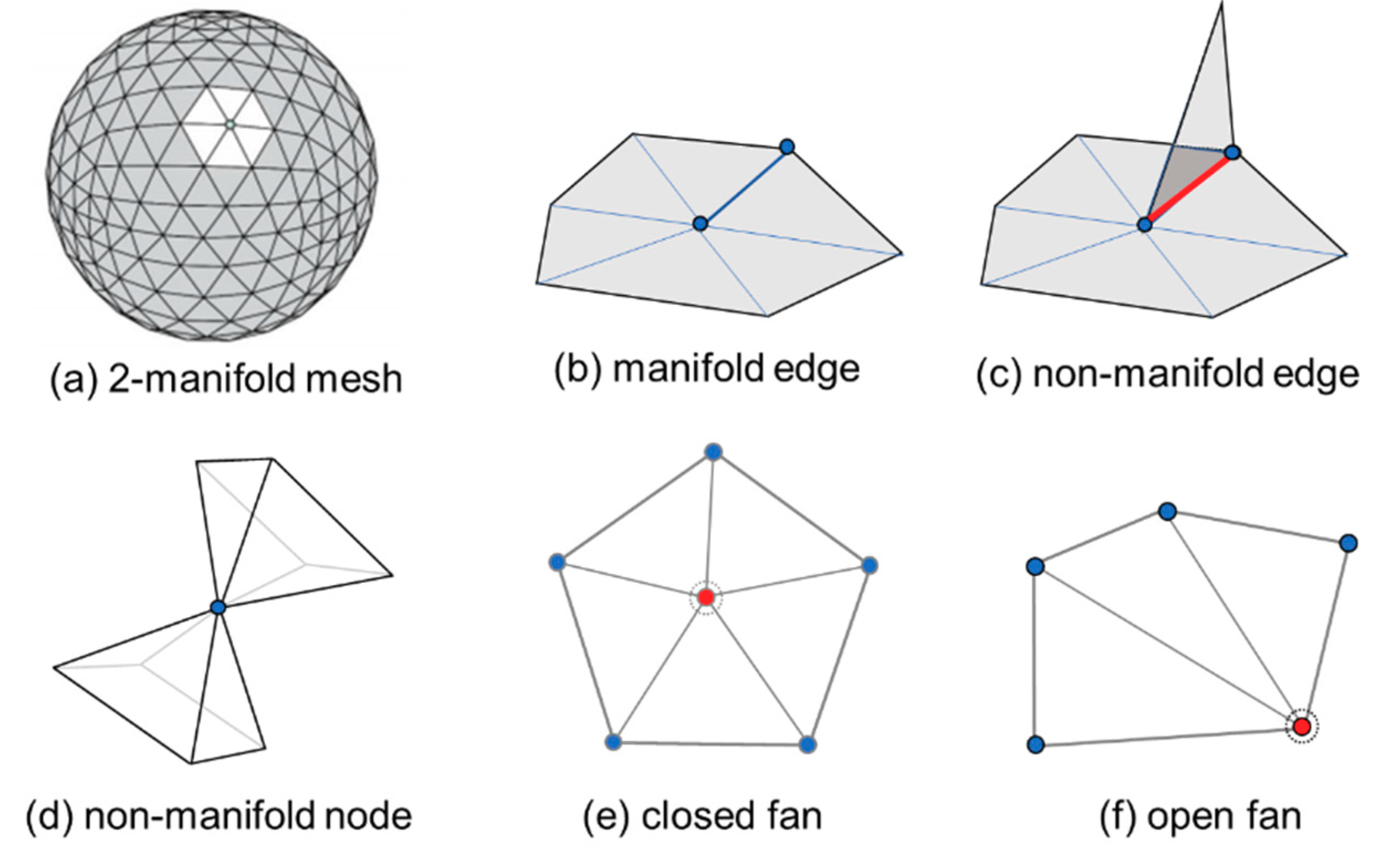
Figure 1.
Manifold definitions: (a) A 3D triangular mesh of a sphere with 512 triangles; (b) Manifold edge; (c) Non-manifold edge; (d) Non-manifold node; (e) Closed fan; (f) Open fan.
Figure 1.
Manifold definitions: (a) A 3D triangular mesh of a sphere with 512 triangles; (b) Manifold edge; (c) Non-manifold edge; (d) Non-manifold node; (e) Closed fan; (f) Open fan.
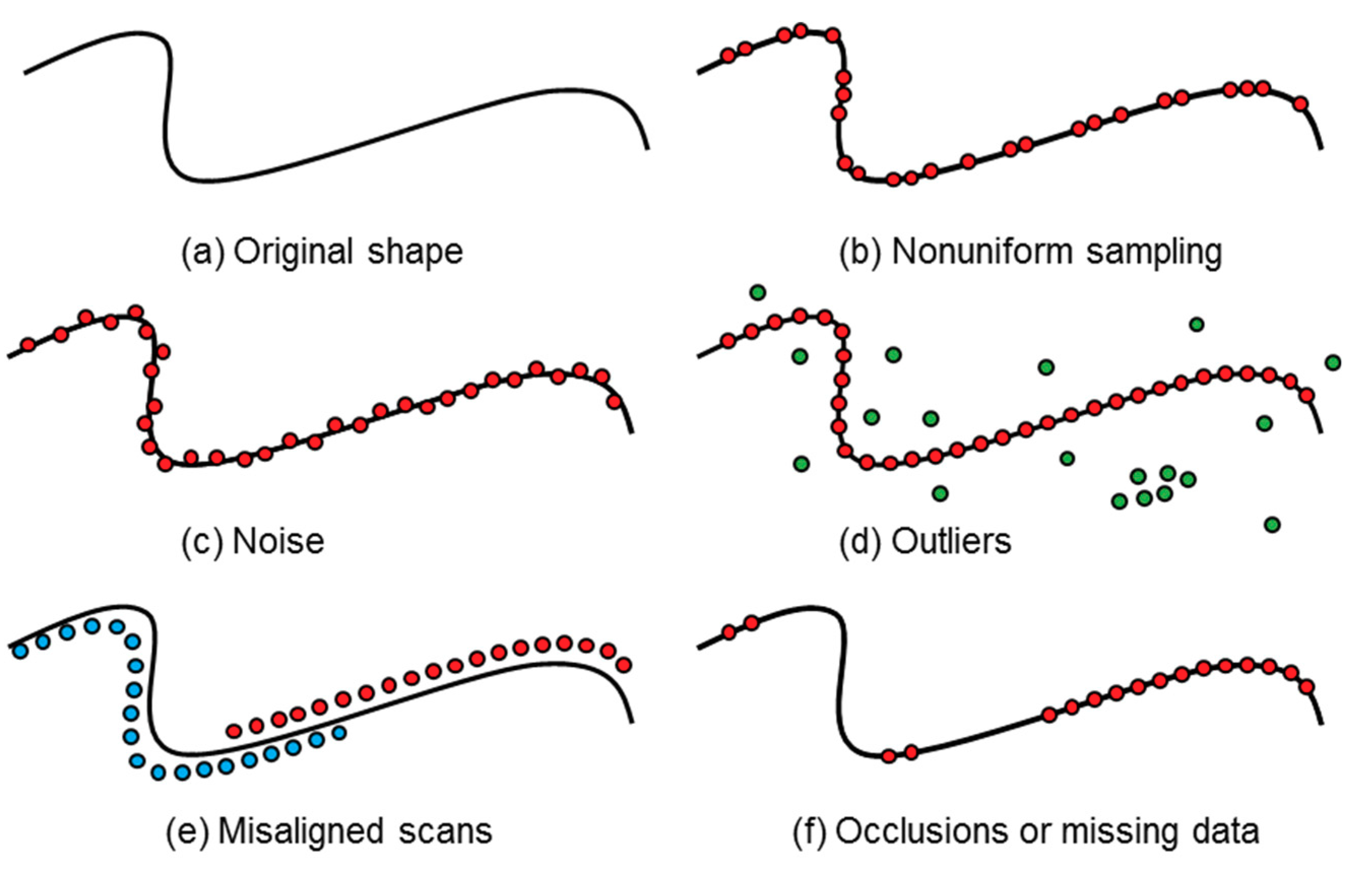
Figure 2.
Common examples of different forms of point cloud artifacts, shown here in the case of a curve in 2D (Modified after [
14]).
Figure 2.
Common examples of different forms of point cloud artifacts, shown here in the case of a curve in 2D (Modified after [
14]).
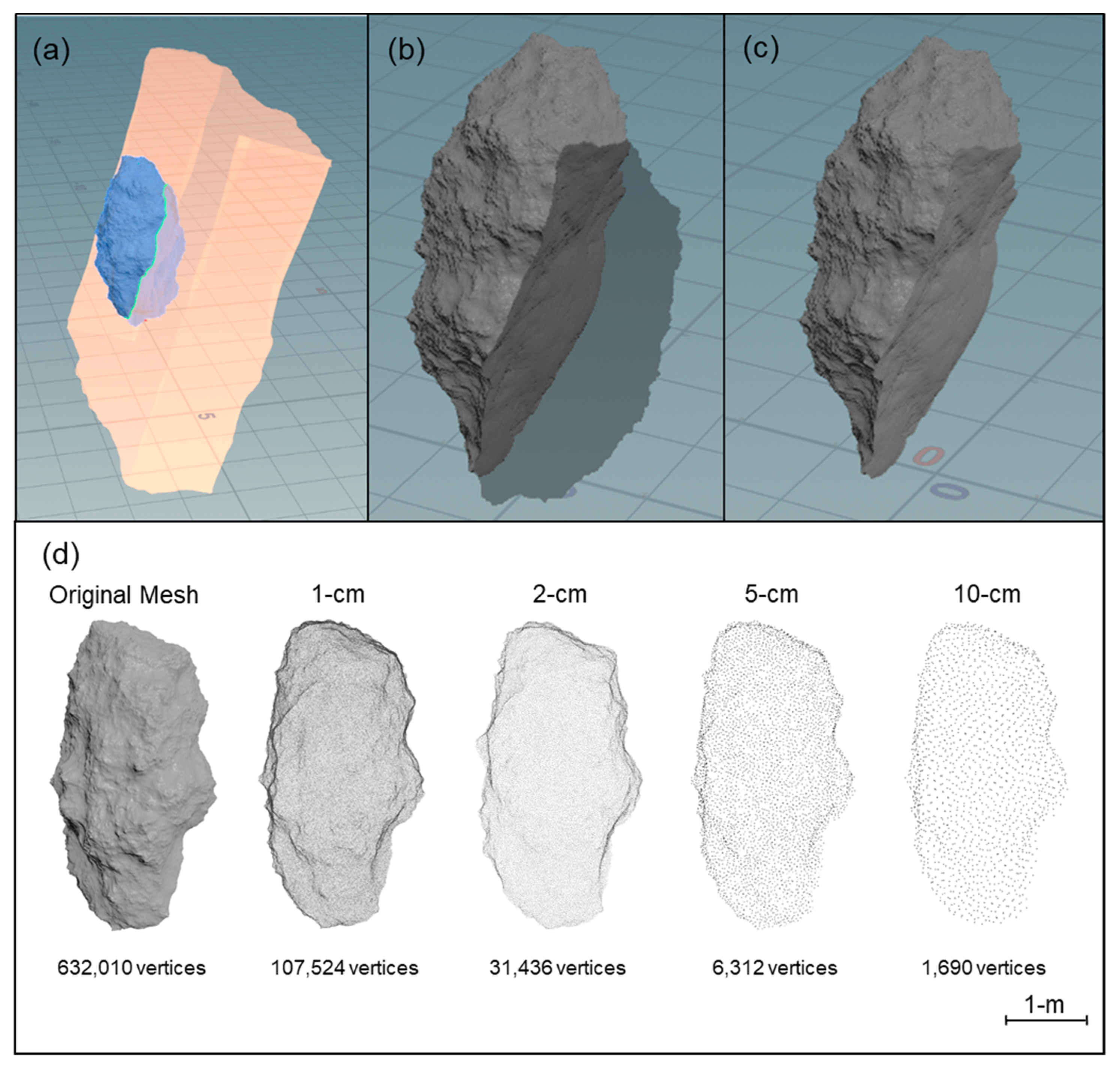
Figure 3.
Generation of the synthetic rockfall object: (a) Procedural geometry generation; (b) Segmented rockfall geometry from a synthetic failure plane; (c) Surface mesh of the rockfall object; (d) Front view of the 3D mesh and resulting subsampled point clouds ranging from 1 cm point spacing to 10 cm point spacing.
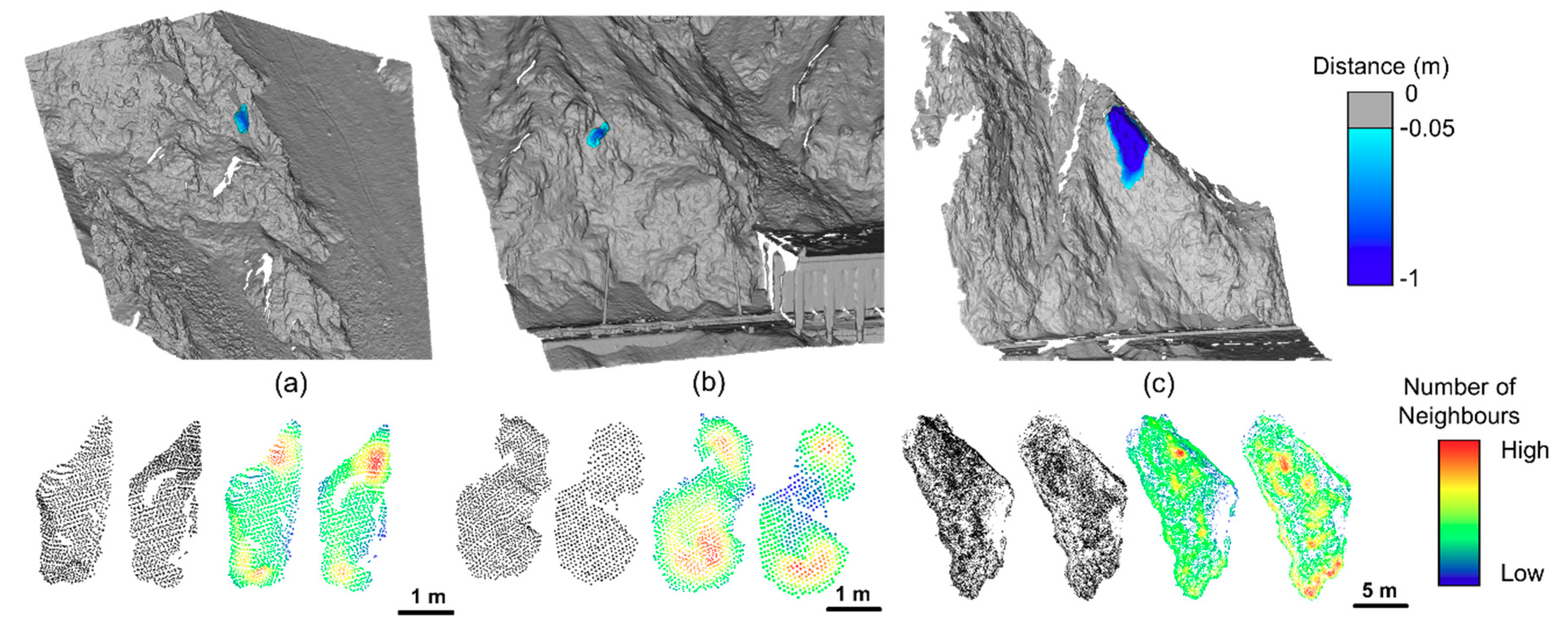
Figure 4.
Overview of the three natural rockfall events used in the study: (a) Rockfall 1: occurred between 2015-10-23 and 2016-02-15; (b) Rockfall 2: occurred between 2015-06-09 and 2015-08-24; (c) Rockfall 3: occurred between 2016-02-15 and 2016-05-01. The black points correspond to the TLS points for the front and back (left to right) of each of the rockfall objects. The colored points correspond to the number of neighbors within a 50 cm diameter sphere. High number of neighbors correspond to the warmer colors while low number of neighbors correspond to the cooler colors.
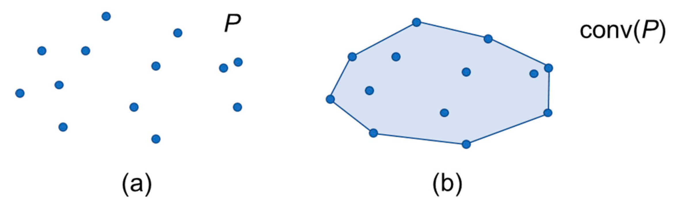
Figure 5.
Overview of a Convex Hull in 2D: (a) input points; (b) Convex Hull of the input point cloud.
Figure 5.
Overview of a Convex Hull in 2D: (a) input points; (b) Convex Hull of the input point cloud.
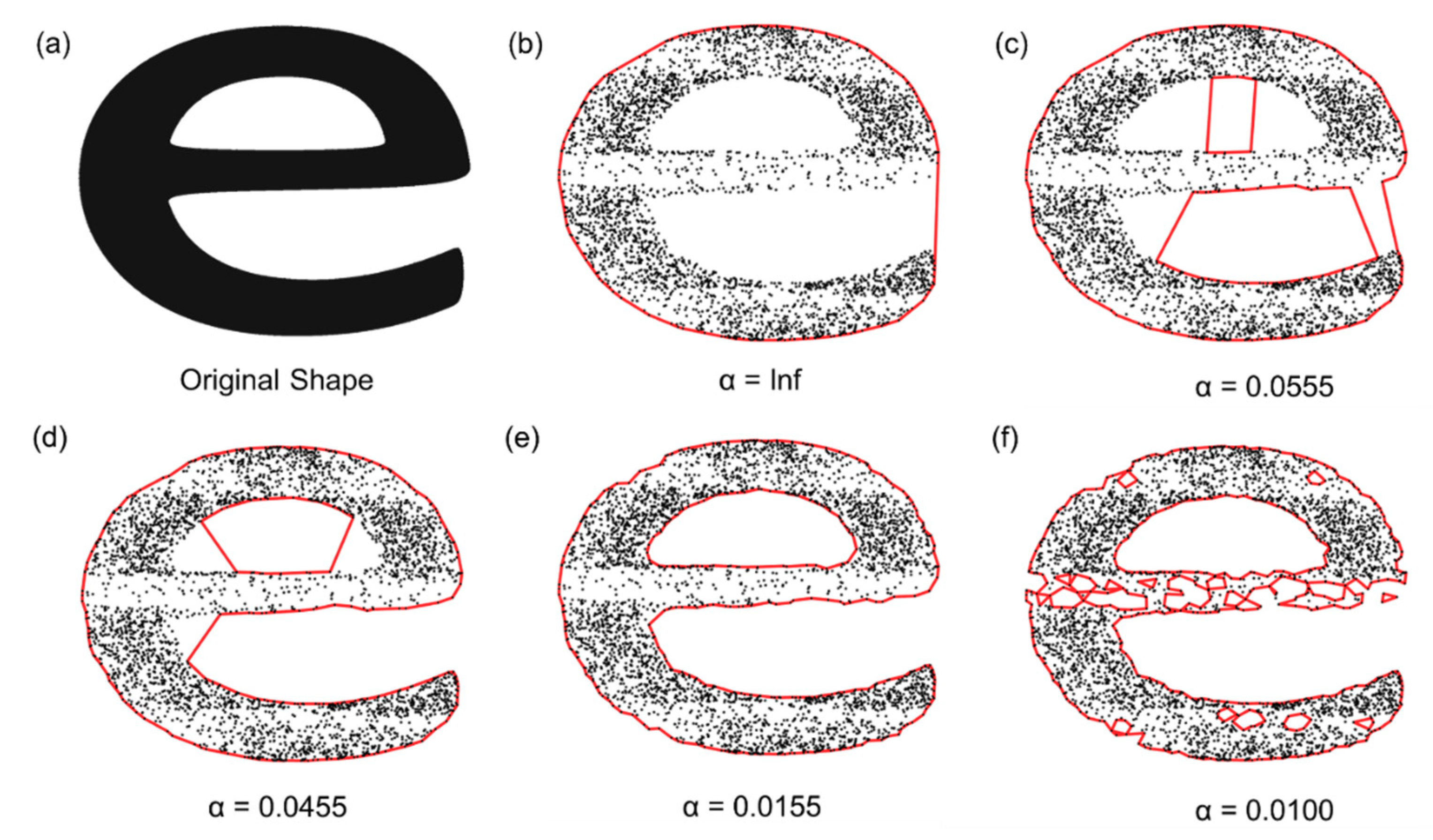
Figure 6.
Illustrative example of Alpha-shapes in 2D: (a) The original shape; (b) A Convex Hull fitted to the data points, representing the case when the Alpha-radius is equal to infinity; (c–e) Refined Alpha-shapes fitted to the data points as the Alpha-radius is decreased; (f) Point at which the Alpha-radius can pass internally thought the data points and the Alpha-shape breaks down into smaller shapes.
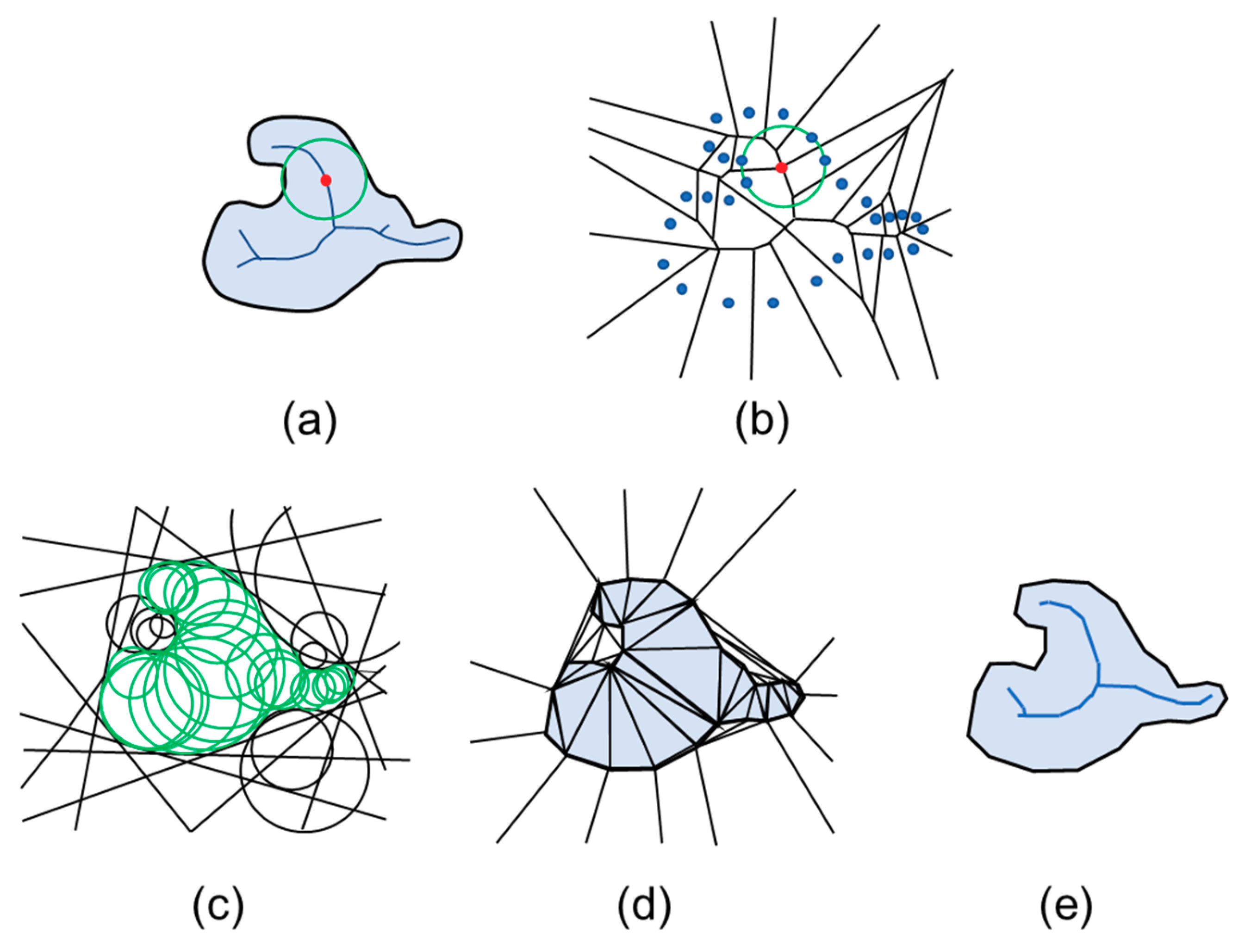
Figure 7.
Overview of the Power Crust approach depicted in 2D: (
a) A solid object with its medial axis depicted in dark blue; one maximal interior ball is shown (green); (
b) The Voronoi diagram of a input point sample from the object surface, with the Voronoi ball surrounding one pole shown; (
c) The inner and outer polar balls; (
d) The labeled inner and outer power diagram cells of the poles; (
e) The Power Crust and the power shape of its interior solid. (Adapted from [
21]).
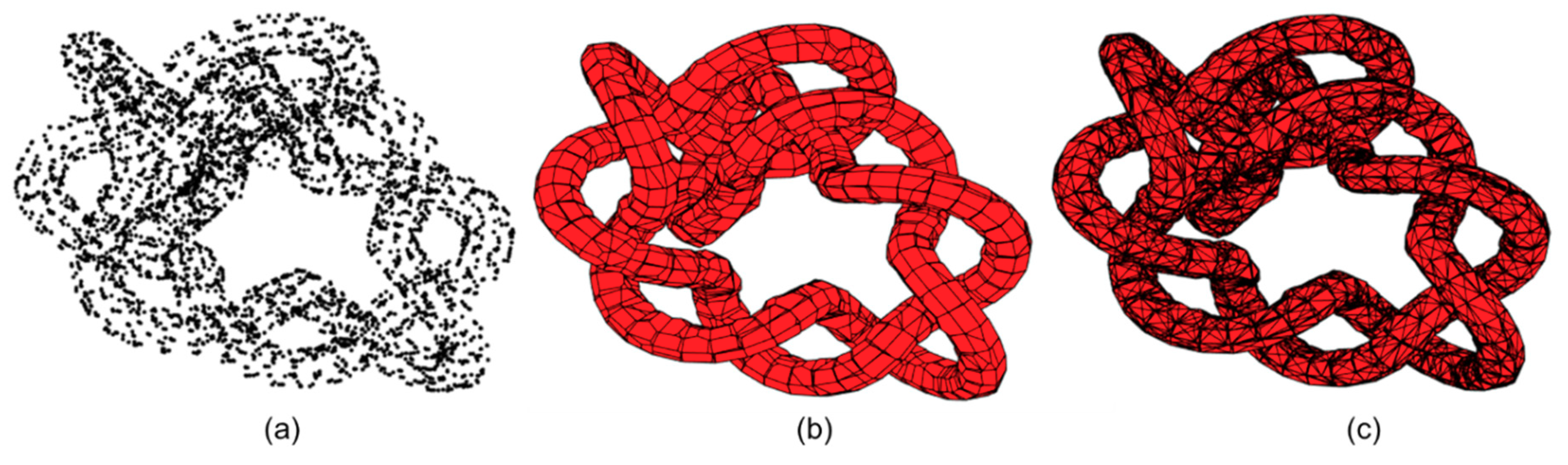
Figure 8.
Example of Power Crust implementation: (a) Input knot point cloud; (b) Power Crust polygonal surface mesh; (c) Refined triangulated Power Crust surface mesh.
Figure 8.
Example of Power Crust implementation: (a) Input knot point cloud; (b) Power Crust polygonal surface mesh; (c) Refined triangulated Power Crust surface mesh.
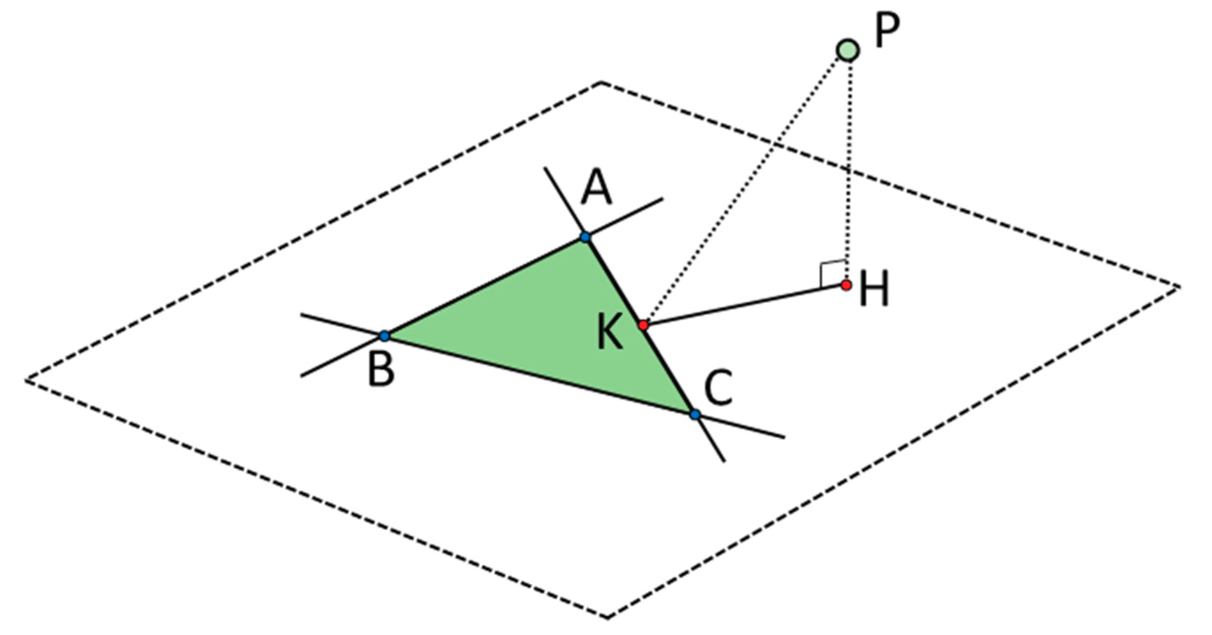
Figure 9.
Distance calculation between point
P and triangle
ABC (Modified from [
22]).
Figure 9.
Distance calculation between point
P and triangle
ABC (Modified from [
22]).
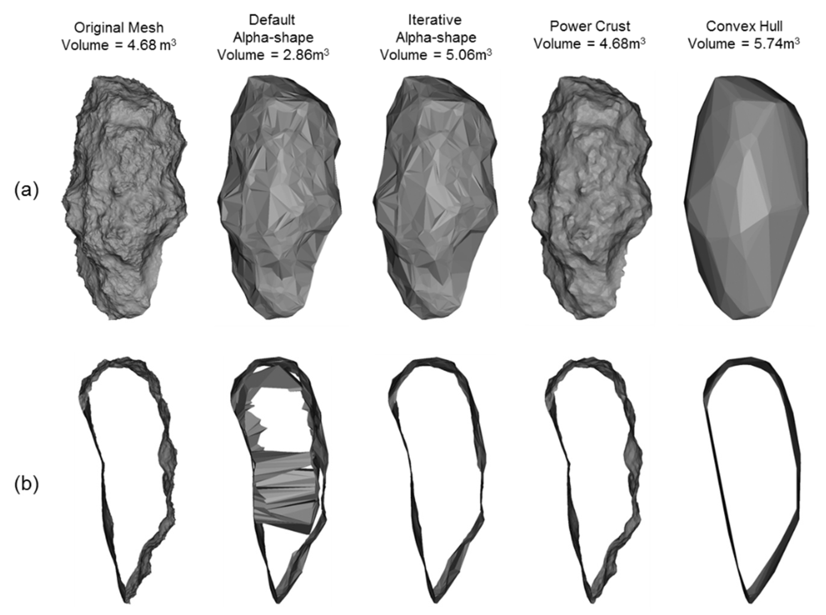
Figure 10.
Surface reconstruction for the synthetic rockfall object: (a) Triangulated surface meshes for each surface reconstruction algorithm; (b) Cross sections through the triangulated surface meshes. Note that the default Alpha-shape produces a reconstruction with boundary facets within the object.
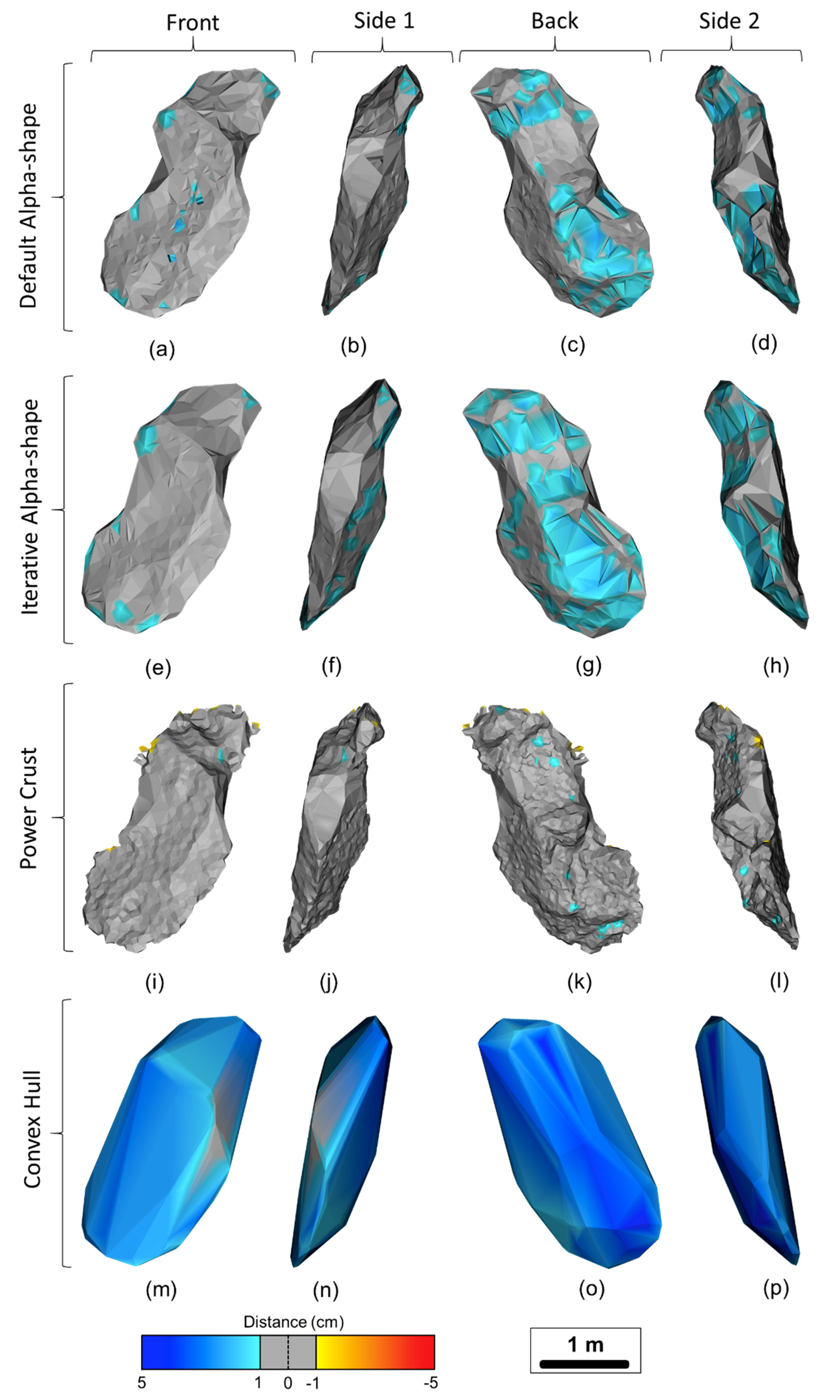
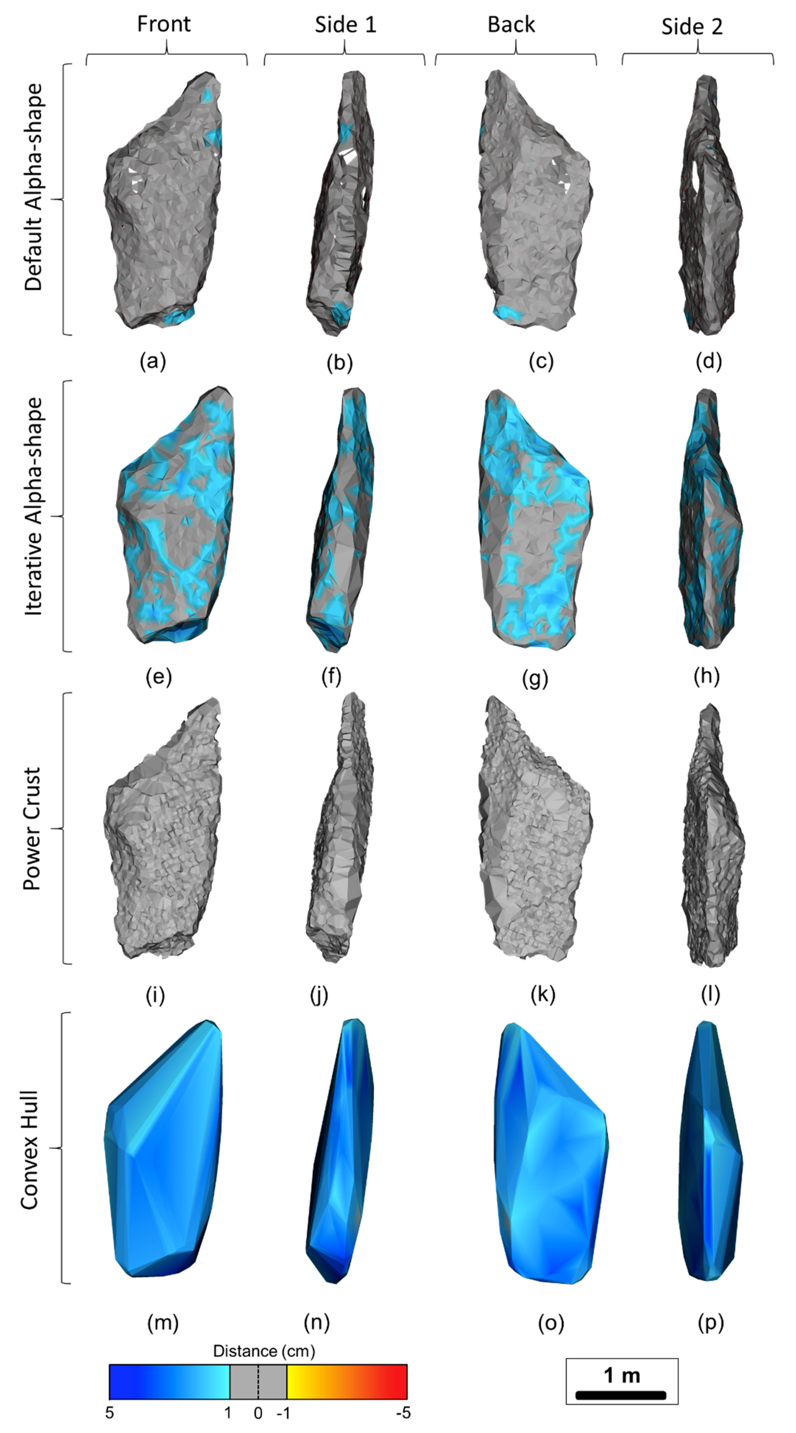
Figure 11.
Distance computations for Rockfall 1 using the four reconstruction methods and displaying the four sides of the rockfall objects after 90-degree clockwise rotation.
Figure 11.
Distance computations for Rockfall 1 using the four reconstruction methods and displaying the four sides of the rockfall objects after 90-degree clockwise rotation.
Figure 12.
Distance computations for Rockfall 2 using the four reconstruction methods and displaying the four sides of the rockfall objects after 90-degree clockwise rotation.
Figure 12.
Distance computations for Rockfall 2 using the four reconstruction methods and displaying the four sides of the rockfall objects after 90-degree clockwise rotation.
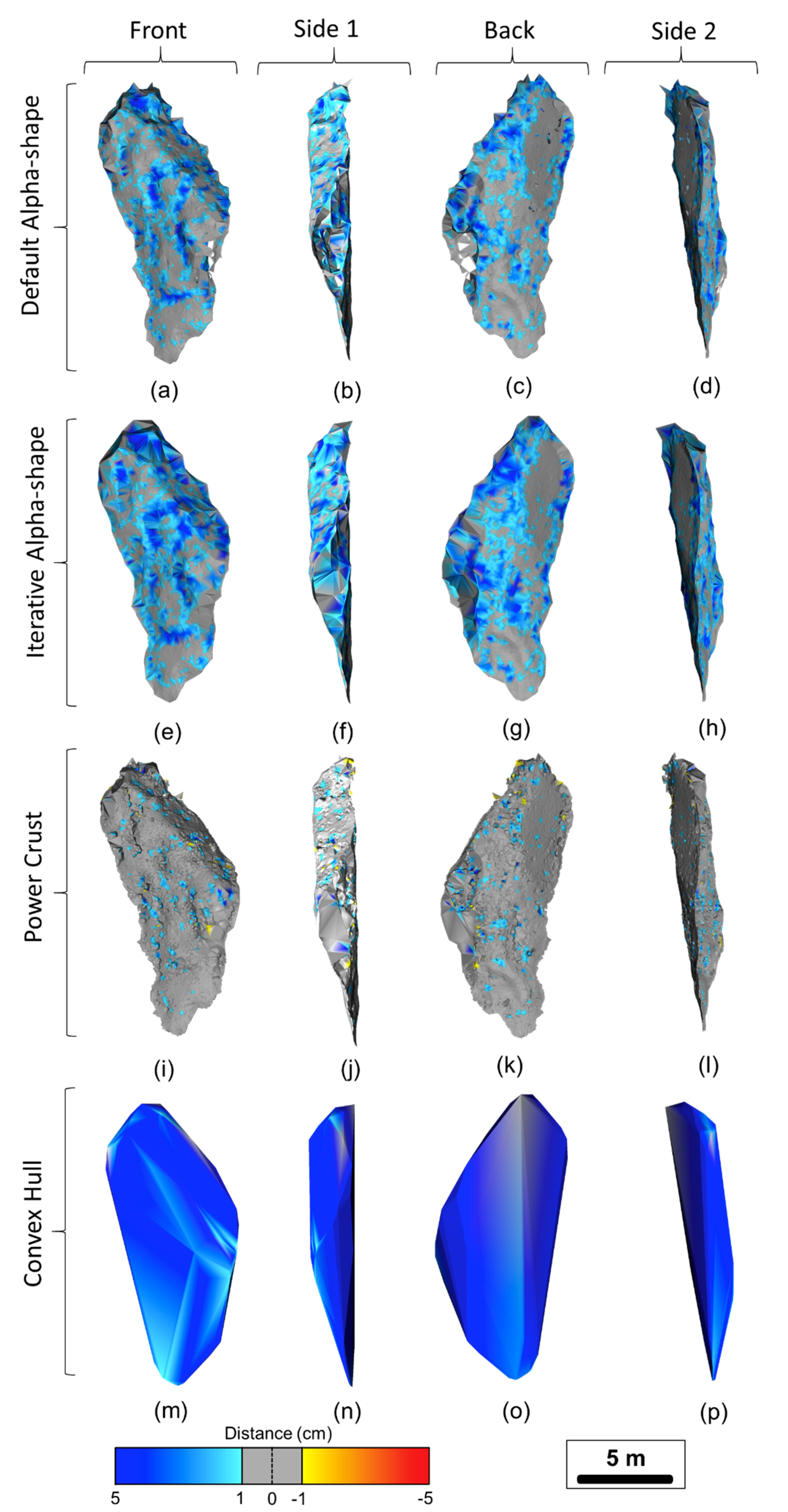
Figure 13.
Distance computations for Rockfall 3 using the four reconstruction methods and displaying the four sides of the rockfall objects after 90-degree clockwise rotation.
Figure 13.
Distance computations for Rockfall 3 using the four reconstruction methods and displaying the four sides of the rockfall objects after 90-degree clockwise rotation.
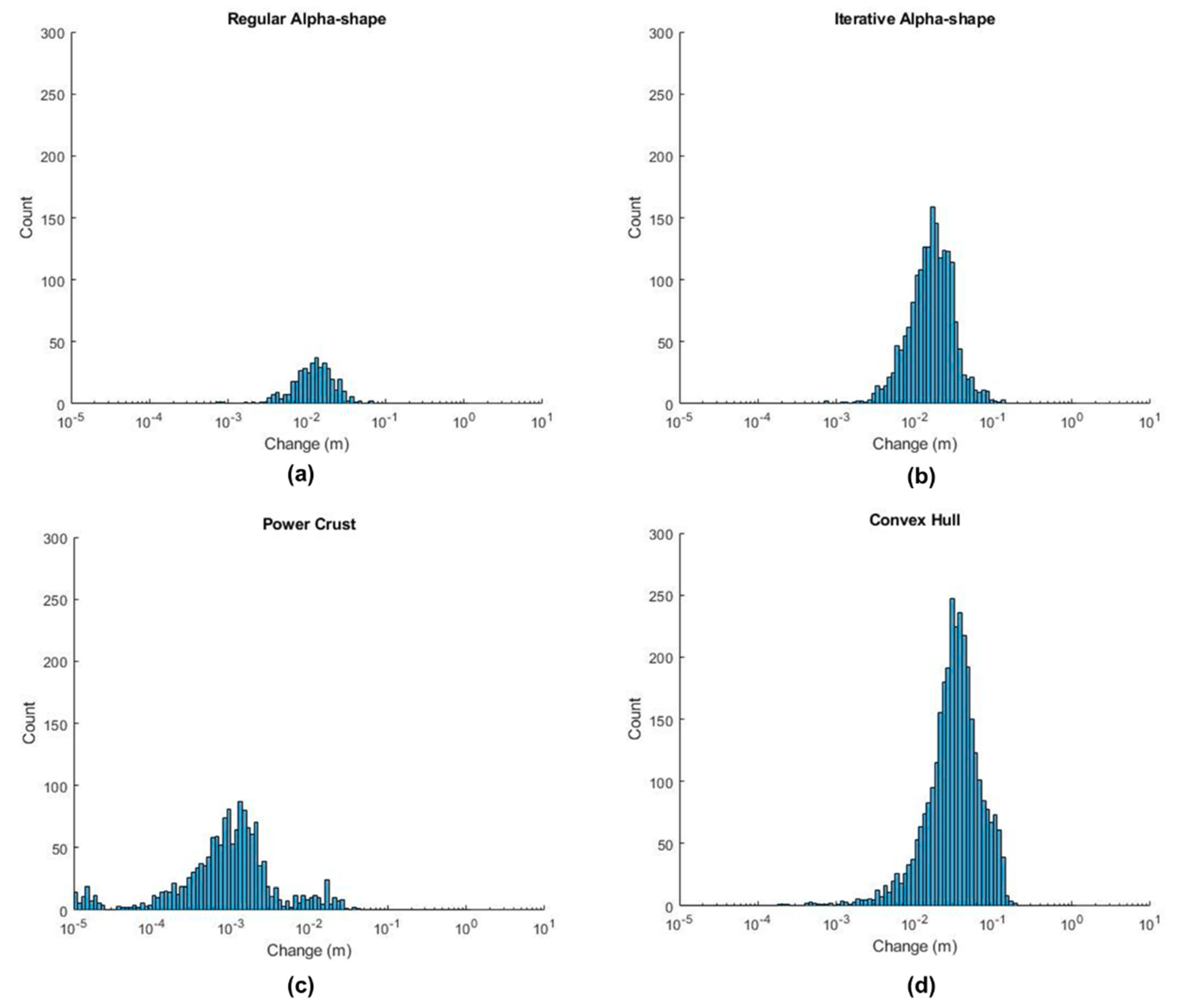
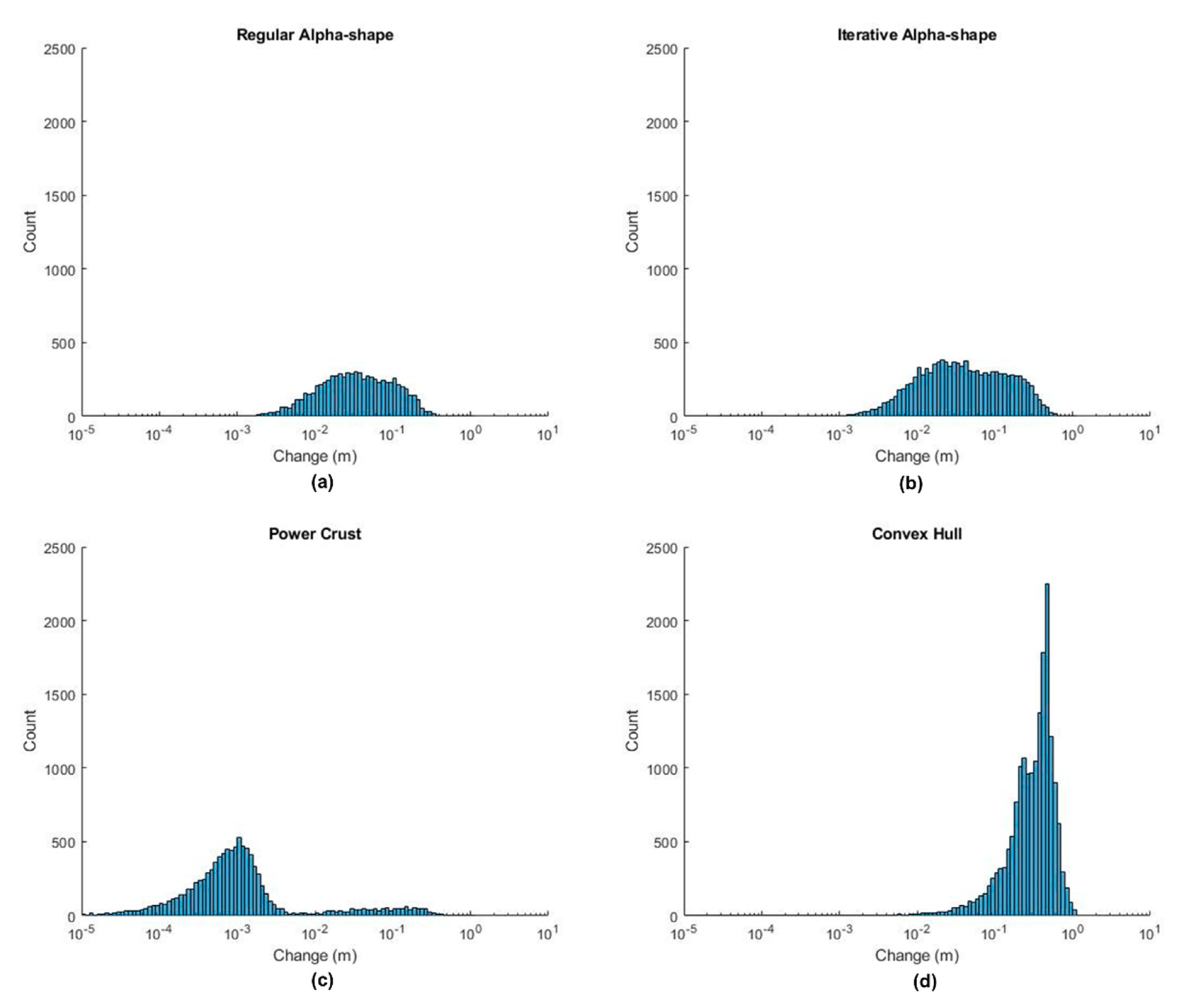
Figure 14.
Histograms displaying deviation of the mesh from the input point cloud for each of the surface reconstruction methods for Rockfall 1: (a) Regular Alpha-shape. (b) Iterative Alpha-shape. (c) Power Crust. (d) Convex Hull.
Figure 14.
Histograms displaying deviation of the mesh from the input point cloud for each of the surface reconstruction methods for Rockfall 1: (a) Regular Alpha-shape. (b) Iterative Alpha-shape. (c) Power Crust. (d) Convex Hull.
Figure 15.
Histograms displaying deviation of the mesh from the input point cloud for each of the surface reconstruction methods for Rockfall 2: (a) Regular Alpha-shape. (b) Iterative Alpha-shape. (c) Power Crust. (d) Convex Hull.
Figure 15.
Histograms displaying deviation of the mesh from the input point cloud for each of the surface reconstruction methods for Rockfall 2: (a) Regular Alpha-shape. (b) Iterative Alpha-shape. (c) Power Crust. (d) Convex Hull.
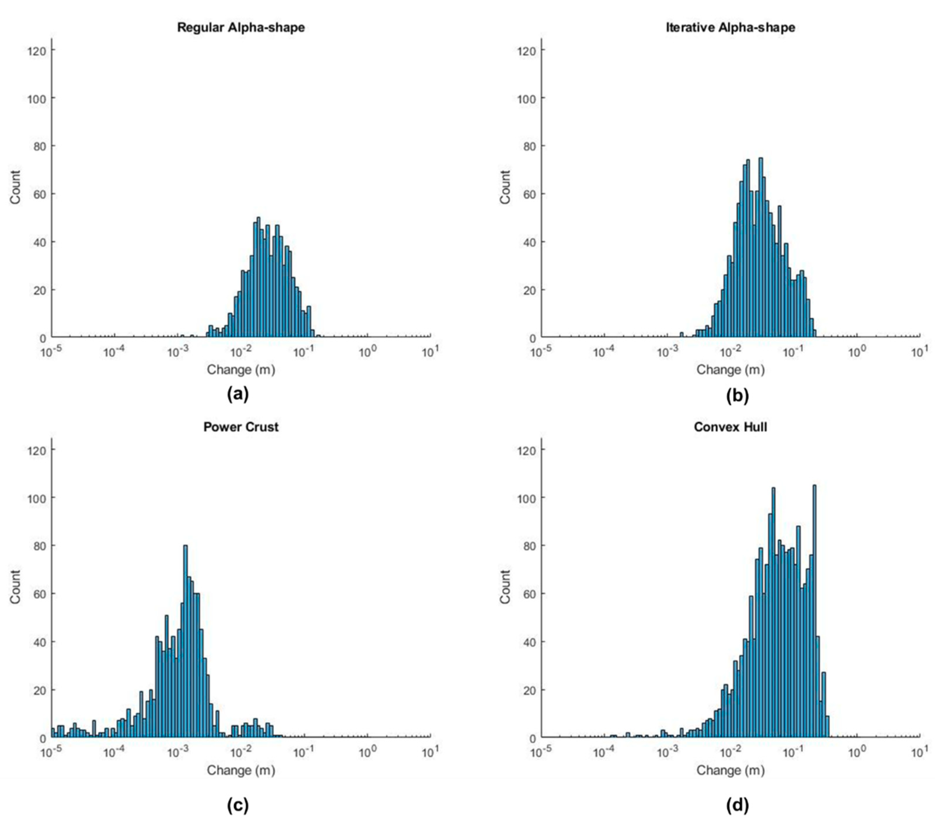
Figure 16.
Histograms displaying deviation of the mesh from the input point cloud for each of the surface reconstruction methods for Rockfall 3: (a) Regular Alpha-shape. (b) Iterative Alpha-shape. (c) Power Crust. (d) Convex Hull.
Figure 16.
Histograms displaying deviation of the mesh from the input point cloud for each of the surface reconstruction methods for Rockfall 3: (a) Regular Alpha-shape. (b) Iterative Alpha-shape. (c) Power Crust. (d) Convex Hull.
Table 1.
Comparison of the surface reconstruction results for the four different subsampled point clouds of the synthetic rockfall object.
Table 1.
Comparison of the surface reconstruction results for the four different subsampled point clouds of the synthetic rockfall object.
| Point Spacing | Surface Reconstruction Method | Faces | Vertices | Volume (m3) | Volumetric Error (%) | Alpha-Radius (m) |
|---|
| 1-cm | Default Alpha-shape | 43,110 | 20,888 | 1.69 | −63.90 | 0.3841 |
| Iterative Alpha-shape | 21,046 | 10,525 | 5.18 | 10.65 | 0.62619 |
| Power Crust | 954,648 | 464,855 | 4.68 | −0.02 | N/A |
| Convex Hull | 1182 | 593 | 5.87 | 25.39 | Inf. |
| 2-cm | Default Alpha-shape | 16,782 | 8063 | 2.08 | −55.63 | 0.4307 |
| Iterative Alpha-shape | 10,500 | 5244 | 4.54 | −2.93 | 0.56824 |
| Power Crust | 338,322 | 166,774 | 4.68 | −0.01 | N/A |
| Convex Hull | 782 | 393 | 5.83 | 24.57 | Inf. |
| 5-cm | Default Alpha-shape | 5940 | 2866 | 2.86 | −38.82 | 0.493 |
| Iterative Alpha-shape | 4392 | 2198 | 5.06 | 8.09 | 0.59193 |
| Power Crust | 71,822 | 35,646 | 4.68 | −0.09 | N/A |
| Convex Hull | 514 | 259 | 5.74 | 22.69 | Inf. |
| 10-cm | Default Alpha-shape | 2354 | 1157 | 3.62 | −22.73 | 0.5377 |
| Iterative Alpha-shape | 2070 | 1035 | 4.75 | 1.40 | 0.58245 |
| Power Crust | 18,644 | 9261 | 4.66 | −0.40 | N/A |
| Convex Hull | 364 | 184 | 5.62 | 20.00 | Inf. |
Table 2.
Surface reconstruction results for Rockfall 1.
Table 2.
Surface reconstruction results for Rockfall 1.
| Surface Reconstruction Method | Faces | Vertices | Holes | Volume (m3) |
|---|
| Default Alpha-shape | 6746 | 2937 | 30 | 0.25 |
| Iterative Alpha-shape | 2922 | 1464 | 0 | 1.34 |
| Power Crust | 37,412 | 18,597 | 0 | 1.45 |
| Convex Hull | 310 | 157 | 0 | 1.82 |
Table 3.
Surface reconstruction results for Rockfall 2.
Table 3.
Surface reconstruction results for Rockfall 2.
| Surface Reconstruction Method | Faces | Vertices | Holes | Volume (m3) |
|---|
| Default Alpha-shape | 2848 | 1337 | 11 | 0.94 |
| Iterative Alpha-shape | 1668 | 836 | 0 | 1.63 |
| Power Crust | 28,704 | 14,076 | 0 | 1.39 |
| Convex Hull | 222 | 113 | 0 | 2.44 |
Table 4.
Surface reconstruction results for Rockfall 3.
Table 4.
Surface reconstruction results for Rockfall 3.
| Surface Reconstruction Method | Faces | Vertices | Holes | Volume (m3) |
|---|
| Default Alpha-shape | 21,640 | 10,492 | 46 | 57.20 |
| Iterative Alpha-shape | 13,368 | 6688 | 0 | 129.63 |
| Power Crust | 183,044 | 90,359 | 0 | 123.81 |
| Convex Hull | 226 | 115 | 0 | 211.77 |
Table 5.
Descriptive statistics for the distance computations for each surface reconstruction method for Rockfall 3.
Table 5.
Descriptive statistics for the distance computations for each surface reconstruction method for Rockfall 3.
| Surface Reconstruction Method | Mean (m) | Standard Deviation (m) | Variance (m) | Skewness |
|---|
| Default Alpha-shape | 0.0017 | 0.0055 | 3.02 * 10−5 | 4.22 |
| Iterative Alpha-shape | 0.011 | 0.015 | 2.12 * 10−4 | 2.36 |
| Power Crust | 4.8 * 10−5 | 0.0047 | 2.22 * 10−5 | 0.10 |
| Convex Hull | 0.038 | 0.029 | 8.62 * 10−4 | 1.39 |
Table 6.
Descriptive statistics for the distance computations for each surface reconstruction method for Rockfall 2.
Table 6.
Descriptive statistics for the distance computations for each surface reconstruction method for Rockfall 2.
| Surface Reconstruction Method | Mean (m) | Standard Deviation (m) | Variance (m) | Skewness |
|---|
| Default Alpha-shape | 0.013 | 0.023 | 5.3 * 10−4 | 2.32 |
| Iterative Alpha-shape | 0.025 | 0.036 | 0.0013 | 2.12 |
| Power Crust | −5.1 * 10−5 | 0.0060 | 3.6 * 10−5 | −2.35 |
| Convex Hull | 0.078 | 0.072 | 0.0052 | 1.17 |
Table 7.
Descriptive statistics for the distance computations for each surface reconstruction method for Rockfall 3.
Table 7.
Descriptive statistics for the distance computations for each surface reconstruction method for Rockfall 3.
| Surface Reconstruction Method | Mean (m) | Standard Deviation (m) | Variance (m) | Skewness |
|---|
| Default Alpha-shape | 0.024 | 0.048 | 0.0023 | 2.97 |
| Iterative Alpha-shape | 0.051 | 0.088 | 0.0078 | 2.74 |
| Power Crust | 0.0062 | 0.040 | 0.0016 | 6.0056 |
| Convex Hull | 0.35 | 0.19 | 0.036 | 0.52 |


