Abstract
Law enforcement agencies (LEA) have long attempted to determine crime patterns, determinants of crime, and ways to improve security. For several years, LEAs have utilized geographic information systems (GISs) to better understand the spatial nature of crimes and possible spatiotemporal patterns. While previous analyses have yielded spatial clusters of high crime areas (i.e., hot spots), these analyses have lacked specificity at the street level. This research builds on the concept of a hot spot area and creates linear statistically significant spatial crime clusters at the street level, namely hot streets. The identification of hot streets has the potential to assist LEAs in reducing crime through increased patrolling and refocusing efforts at the street level. This study created a GIS-based geoprocessing model to analyze different crime types at varying temporal scales and in different cities (Atlanta, Georgia and Houston, Texas), classifying streets based on four crime cluster confidence levels. The research found that the geoprocessing model successfully streamlined the creation of crime hot streets in the two study areas, led to the development of multi-scale hot street maps, and can be used and edited by anyone who wants to perform linear cluster analysis in other topics.
1. Introduction
Crime, like any other event, always occurs at a particular place and time. Geographic information systems (GISs) have been used by law enforcement agencies (LEAs) to help their crime analysis divisions visually represent and understand crime patterns over space and time. Currently, there is a two-part classification of crimes, but only Part I offenses were used for this research since they include spatial information on where they occurred. Part I offenses include eight crime types, namely criminal homicide, rape, robbery, aggravated assault, burglary, larceny, auto theft, and arson. Based on a variety of crime theories, there are several methods that one can employ for crime analysis which aid in crime reduction efforts by LEAs, especially within high crime areas. Brantingham’s crime pattern theory deals with crime–place association that leads to the generation of these high crime areas. The theory explains that crimes are not random, and they do not occur uniformly in time, space, or society [1]. This has led geospatial crime analysts to use spatial analysis and statistic tools to perform crime analysis and determine the high crime areas and spatial or temporal patterns. Using the Part I crimes, studies have mainly concentrated on mapping crime point density, kernel density, hot spot, and heat maps while finding correlations with the help of R and R-ArcGIS Bridge, or other statistical software [2,3,4]. One of the most popular methods of the listed techniques is hot spot analysis. Hot spots are defined as smaller areas that suffer from statistically significant clusters of crime.
Hot spot policing has become a common way for police departments to prevent crime [5]. Recently, results of studies have supported the assertion that focused police efforts on hot spots can be effective in preventing crime [5,6,7,8,9,10]. In a national survey sample of police departments with over 100 officers, 62% reported using crime mapping to identify crime hot spots for concentrated efforts [11]. In 2016, 17 systematic reviews of policing performed for more than 13 years concluded that most of the effective policing strategies regarding crime control concentrated on small geographic areas [12]. Systematic reviews are relevant because they provide an assured test of strategy effectiveness, which is an essential resource in academia, criminology, and police practitioner interests [12]. Though current neighborhood hot spot methods fulfill their goal of visually representing crime occurrences and helping LEAs and civilians be aware of what is happening around them, they lack an accurate representation at the street level. This is because crime concentrates and is stable at a micro-scale/minimal units of geography [13,14,15], and there is an increased chance to miss important crime variation in higher geographic units [14]. When crime concentrates at certain places to form hot spots on the micro-scale such as streets, these high crime segments are called hot streets. Hot street creation often happens at the neighborhood level to provide the missing degree of high precision for observing crimes [16]. The criminology of a place has reveals many times that there are high crime streets in low-crime neighborhoods and low crime streets in high-crime neighborhoods [17]. As a few streets contain the majority of crime, studies have shown that patrols of hot spots in those neighborhoods and the remainder of the city have resulted in reductions in crime [5,18]. Since there has been no easy way of delineating linear hot spots, also known as hot streets [19], this research provides a way to efficiently replicate the creation of hot spots at a street-level as hot streets.
Currently, there are several techniques used for the identification of hot streets for policing, as no single method is sufficient and a majority of the methods are not straight forward [19]. As seen in several examples [4,14,19,20], most of the current street analyses of crime patterns include the use of total crime count by street symbolized in several ways including point density raster attachment. There are several ways to use statistics to find spatial clusters, e.g., Moran’s I, local Moran’s I, Geary’s C, Getis Ord Gi, and Getis Ord Gi* [3]. For a hot street analysis to be a significant measure of crime clusters like the hot spot analysis tool, it has to utilize a GIS and apply spatial statistical tests to ensure that the clustering is not a result of random chance [21]. Currently, the local Moran’s I approach has been used to find the spatial autocorrelation between streets in order to display hot streets [14]. This research delves into the creation of a model that uses a different correlation method called the Getis Ord Gi* statistic. The Getis Ord Gi* is a very popular statistic used in finding hot spots between polygon and point features. Both the Gi* statistic and the local Moran’s I are significant measures of local spatial clusters, but they vary in how they are calculated [22]. For the local Moran’s I, the value for the feature (street) being analyzed is not included in the analysis, as only the value of the nearby features determine the result. The Getis Ord Gi* takes account the value of each feature, including the feature being analyzed, to find the clusters. Both methods are expected to have some similarities in the results, but there are also a few differences. By developing a method to use the Gi* statistic in this research, future work can be performed to see which methods of correlation will yield the best micro-scale results.
Though the Gi* statistic is widely used for hot spots, there are a lack of publications that utilize the statistic on the street level. There is only one methodology [23] that describes how to utilize the Gi* statistic on the street level. This work fills the knowledge gap of hot street development through the addition of a Gi* clustering algorithm that that adds spatial statistical values. The Getis Ord Gi* statistic is used in this research because it takes account of the feature being analyzed, as well as the neighboring features, to locate where high (hot street) and low (cold street) values spatially cluster and show local dependence [24]. In addition to previous work, this study uses modified procedures and provides a model for others.
The primary research goal is to further studies on the creation of hot streets within a GIS through the development of an efficient model that uses the Getis Ord Gi* statistic. The Getis Ord Gi* delineates statistically significant spatial clusters once the crimes are attached to the nearest streets. This method should provide LEAs with a more in-depth and geographically localized result. The hot streets model created in this work is used at multiple scales within the study areas of Atlanta, Georgia and Houston, Texas to examine street-level relationships of crime. Clusters of high and low values were visualized and statistical significance was determined through the z-scores and p-values that display spatial clusters of streets with high and low occurrences of crime. This research presents an automated model for achieving the set goal, enabling people of all experiences and levels to perform analysis. The resulting method could lead to safer travel for civilians, reduced crime along the streets within those hot spot areas, and more precise street segments within regions for police intervention, and better allocation of police resources [14].
2. Materials and Methods
The modeling of crime hot streets incorporates established methods and newer analysis techniques that require a wide variety of geoprocessing tools. These methods were formulated after a critical review of relevant literature and informed the development of the model outlined in this section. While the model described here is based in ArcGIS Pro v2.2, the processes can be modified and applied within any geographic information system that supports the described geospatial analyses.
2.1. Study Area
This research developed its model and performed the analysis in the cities of Atlanta, Georgia, and Houston, Texas (see Figure 1). The city of Atlanta is the capital of the state of Georgia and consists of 498,000 people [25]; it currently has over 2000 sworn police officers [26], making Atlanta’s police department the largest law enforcement agency in the state of Georgia. The city of Houston has the fourth largest population in the USA with 2.3 million people and approximately 5000 sworn police officers in the department [25,27], making it one of the largest police departments in the United States.
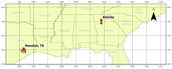
Figure 1.
Map showing study areas.
2.2. Data Selection and Sources
The data were acquired from government and public sector sources such as the Atlanta police department, Houston police department, Atlanta Regional Commission, OpenStreetMap (OSM), and the U.S Census Bureau [28,29,30,31,32]. The data include city limits and street shapefiles [32], as well as spreadsheets containing crime data from the police departments [29,30]. The crime data for Atlanta contain 26,000 records for the calendar year of 2017, while that of Houston were samples from July and August in 2018, with a total of 8742 records. Spatial data on rape were not provided because of security reasons. The crime data tables include the offense/incident number, report date, occurrence date, occurrence time, beat (specific areas that police officers patrol), address, coordinates, uniform crime report (ucr) number, and offense type.
The determining factor in the fitness-for-use of crime data is the ability to integrate it within a GIS for quick automated spatial processing. The crimes already have latitude and longitude positions, which provide a means to quickly integrate the data into a model. The data are credible, as they were provided by the police department, but there have been concerns about spatial accuracy and where the crimes were reported to occur when snapped to the streets. Performing a random sampling of the dataset to nearest street connections provided a numeric value of accuracy to address the connection concerns in using personally non-geocoded data. A random sampling of all crimes at 95% confidence level with a 4% interval needs a sample size of 579. The random sampling showed an over 81% match rate based on addresses of the streets and crimes, but the data were still used because the priority in this model is to join the crime to the closest street of its occurrence. The model successfully matched the crimes to the correct streets based on proximity. The addresses did not match between some of the crimes and streets, because some of the crimes occurred in parking lots and alleys that were given the address of the building they belonged to. Thus, the model places the crime on the street that runs through the alleys, but the crime address is still the same. It would be worthwhile to geocode the data in future studies to ensure that crimes are placed on the correct properties/parcels.
2.3. Research Design
Early crime street mapping techniques, the results of previous research, and case studies of point-to-polyline mapping were the building blocks of this research design. The flow chart in Figure 2 summarizes the seven major steps of the process, which are expanded upon below. The first step of this project is the combination of the crime points to the street segments. One recommended option is to plot crime incident locations on a map and match them to the nearest street layouts based on an approximate distance [9,33]. Other crime-to-street matching techniques may include a direct match between street names, but this might be a problem if the street names in the crime address do not match. This research plotted the crime incident locations and matched them to the nearest streets. Joining the points to the street segments yields a count of points per street segment. This research took this approach a step further by calculating total crime count per mile of the street to account for different street lengths. Afterwards, the hot spot analysis tool was run.
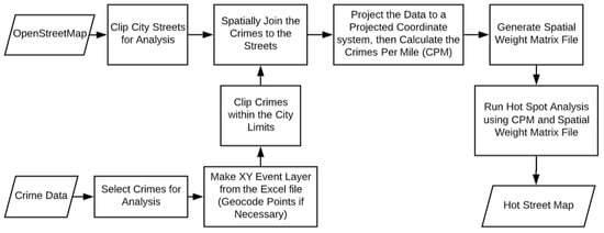
Figure 2.
Flowchart of the hot street model.
The hot spot tool operates based on the null hypothesis of complete spatial randomness and presents results that reject the null hypothesis and show the spatial patterns of crime. The creation of the spatial weights matrix file is essential to determine the scale of analysis and calculating the spatial autocorrelation of the data is compulsory before calculating the Getis Ord Gi* statistic via the hot spot analysis. The scale of analysis for each street in this study included only the intersecting streets, but it has the potential to include streets connected by drive time, walk time, or proximity. The spatial autocorrelation was performed using the Moran’s I statistic to ensure the data show results that indicate clustering that is not a result of random chance.
2.4. Model Procedures
After gathering a general understanding of the appropriate approaches, this section expatiates on three steps from the flowchart (Figure 2).
2.4.1. Select City Streets Excluding Expressways
The extraction of the needed street layer within the study area was the first step of the analysis and made the first sub-model. Following the creation of the street layer within the study area was the removal of expressways and exit ramps. Expressways are patrolled differently, only a handful of crimes occur on them, and they are not connected to neighboring streets. The crimes that occur on the expressways were also removed from the crime data.
2.4.2. Generate Spatial Weight Matrix (SWM) File
A spatial weight matrix (SWM) file is what holds the number of neighboring streets and the amount of influence the streets will have on the final hot street calculation. Depending on the size of the study area, this file can be manually created or with the aid of tools within a GIS. Within ArcGIS ModelBuilder, this portion of the model runs seven different tools to generate the SWM file, each described below and each that can be programmed separately within a GIS. Without this spatial weight matrix that tells the hot spot tool the neighboring streets, the hot spot tool may select roads that do not intersect. The neighboring issue often arises for several GIS users, because the hot spot tool is dominantly used on point and polygon layers.
The first function performed is the generation of a table of connected streets. If it is a small study area consisting of only a few blocks, this can be done manually. First, assign each street a unique number (we can call this FID). Then, duplicate the FIDs within the column based on the number of neighbors. After that, start a column next to the FID and place the FID of the neighboring streets you desire to be used for the Gi* calculation. Then the last column holds a number between 0 and 1 to show how much influence the street has on the hot street calculation. Manually creating this file becomes more difficult with increasing street numbers and neighbors, and it is therefore more efficient to use a tool within a GIS. Within open source software like QGIS, tools like the Nearest Neighbor Analysis can help create this file. For other software’s such as ArcGIS, the SWM file can be created with the Generate Near Table or the Summarize Nearby tool. The Summarize Nearby tool was tested but not used in the final model because of the 20 min run time for this geoprocessing tool alone, and the Generate Near Table is a tool that has functions that can be found in several GISs. Within the Summarize Nearby tool, all distance types except straight-line distance use ArcGIS Online routing and network services. The distance measurement types include: (1) driving distance; (2) driving time; (3) straight line; (4) trucking distance; (5) trucking time; (6) walking distance; and (7) walking time. After generating the table, make sure that columns are titled correctly so that the GIS software can able to read the data for the spatial statistics.
2.4.3. Spatial Statistics
After creating the SWM file with the weighted neighboring features to consider in the analysis, the Moran’s I statistic is used to ensure that there is perfect randomness in the data. The next step is to apply the Gi* statistic to the data. This can be done multiple ways in different GISs, and it is important to use the SWM file with the desired neighbors. The hot spot tool takes both the SWM file containing all the neighbors and the street file to identify statistically significant spatial clusters of high (hot spots) and low (cold spots) street crimes values with the Getis Ord Gi* statistic. The analysis creates a new output feature class with a z-score, p-value, number of neighbors, and confidence level bin (Gi_Bin) for each street. To be shown as a significant hot street, the street has to have a high value and be surrounded by high values compared to the study area. When there is a large difference to the study area and the difference is not a result of random chance, the street has a significant z-score. This creates the possibility of having a street with high values that is not a significant hot street based on the statistics.
2.5. Runs and Runtime
Several model runs selecting for different crime types and days/times were made to ensure that the model ran smoothly. These use case examples are summarized in Table 1, along with the total run times for each model. As can be observed, the median runtime was 4 min 31 s, and the number of crimes selected did not have much influence on the runtime.

Table 1.
List of different runs, crime counts, and run times.
3. Results
3.1. Hot Street Model
The goal of this project was to develop a standardized and automated process for the geospatial analysis of crime at the street level. After performing over 20 trials, this was accomplished, and a workflow of the generic model is presented below (Figure 3); the detailed ModelBuilder workflow from ArcGIS Pro is presented in Appendix A. There are a total of eleven sub-models (see Appendix A) that execute different functions in the model. The input parameters are displayed in blue for the layers and grey for the expressions. The tools are presented in yellow, while the outputs from the tools are shown in green. The first sub-model consisted of the model parameters and expression for the crime selection, which also appeared when the model is run as a tool within a GIS. Preconditions were set because a single feature class could be used with multiple tools and errors often appeared after a few runs without restrictions.
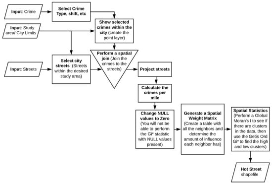
Figure 3.
Hot street sub-model flowchart.
3.2. Spatial Autocorrelation
To ensure the spatial weight matrix contained a minimum of one neighbor in the scale of analysis and the data were randomly dispersed, the Moran’s I tool was run. The Moran’s I spatial autocorrelation tool was used to measure the spatial clustering of both the high values and low values. The results showed high z-scores, which indicates there was clustering and a less than 1% likelihood that the pattern was a result of random chance. The Moran’s I values close to 0 for all runs also indicate that the data were truly randomly dispersed.
3.3. Hot Street Result
After creating the final model, all eight runs displayed different hot streets. The resultant hot streets were categorized into three different confidence levels (CLs) at 90%, 95%, and 99% based on the z-scores and p-values. A 90% confidence level had a p-value < 0.10 and a z-score < −1.65 or > +1.65; a 95% confidence level had a p-value < 0.05 and a z-score < −1.96 or > +1.96; and the 99% confidence level had a p-value < 0.01 and a z-score < −2.58 or > +2.58.
Table 2 shows the total number of hot streets generated from each model run for different street classes and CLs. Service roads had the highest number of hot streets for every run in Atlanta, followed by residential and then tertiary or secondary roads. However, the city of Houston had most of the crimes occur closer to the secondary roads. The hot street maps (see Figure 4, Figure 5, Figure 6 and Figure 7) were placed over kernel density results (Figure 8, Figure 9 and Figure 10) and show that hot streets mostly overlap with high crime kernel density classes (generated using Jenks normal break classification).
Table 2.
Number of hot streets generated from the model.
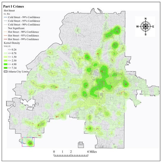
Figure 4.
Hot street map of Part I crimes.
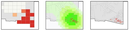
Figure 5.
Zoomed in SW section of the Part I hot street map.
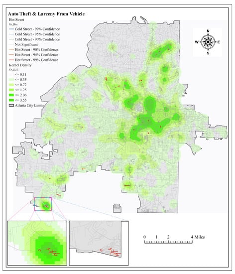
Figure 6.
Hot Street map of auto theft and vehicle larceny.
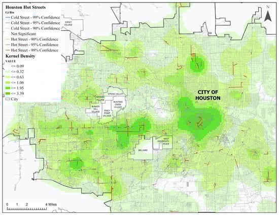
Figure 7.
Part I hot street of western Houston, Texas.
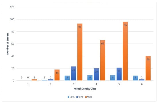
Figure 8.
Part 1 crimes in Atlanta, Georgia.
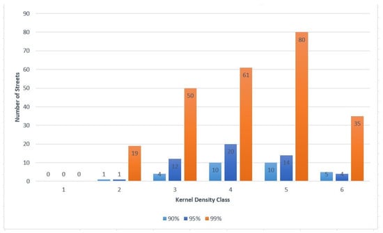
Figure 9.
Auto theft and vehicle larceny.
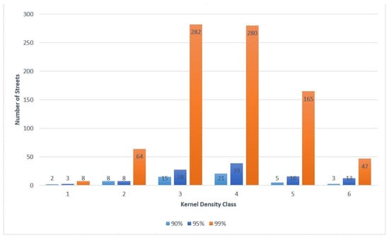
Figure 10.
Part 1 crimes in Houston, Texas.
The results of the hot street analysis of Part 1 crimes in Atlanta showed significant clusters within the highest density classes in Midtown, Downtown, Edgewood, and Princeton Lakes neighborhoods (see Figure 4). It was easier to distinguish hot streets located in the southwest region (Princeton Lakes neighborhood) of Atlanta and the overlap of the hot streets with both a hot spot analysis and kernel density analysis (see Figure 8). The hot street analysis of auto-related crimes in Atlanta yielded significant clusters of hot streets within the Downtown and Princeton lakes neighborhood (Figure 6). An analysis of Part 1 crimes in Houston resulted in significant hot streets Downtown, Midtown, Montrose, Greater Uptown, and Midwest neighborhoods (Figure 7). Figure 8, Figure 9 and Figure 10 show the number of hot streets per kernel density class; most hot streets were found to occur in the higher three density classes in both the city of Atlanta and Houston. Auto-related crimes also showed a higher percentage of hot streets in the in the higher density classes than Part 1 Crimes in Atlanta, and this is discussed further in the next section.
4. Discussion
The model was successful in providing an effective way to evaluate linear spatial clusters and hot streets. The modifiable areal unit problem (MAUP) must be considered here because different aggregation schemes yield different results despite using the same analysis and data [34]. Results that are valid for the street-level crime study may be more accurate than broader area aggregation techniques. Despite the MAUP problem, different results are often valid because different analyses seek to answer different questions on a variety of scales. Hence, practitioners should be aware of this issue and select an appropriate scale of analysis for their analysis when utilizing this model.
4.1. Model
Through the course of developing this model, it was discovered that it could easily be replicated at different scales within different GISs by using the model flowcharts as a guide. After the initial run, the model can be optimized by removing processes that will produce the same result. The sub-model that can be changed is the Generate Spatial Weight Matrix (SWM) sub-model. The sub-model can be removed once the SWM file is created because the table will remain the same if the street layer and the scale of analysis is the same.
The full hot street model can take a considerable amount of time to run, depending on the input parameters of each sub-model. The streets appear to be the primary input that determines the run time of the model. The city of Atlanta had approximately 40,000 streets in the data, and the city of Houston had approximately 120,000 streets. Houston had about three times the number of streets in Atlanta, and the run time from Table 1 shows a three-times increase in the run time. The streets took time to process when linking them with crimes and calculating the crimes per street segment. Overall, within ModelBuilder, the median time of the entire model when using the Generate Near Table tool to create the spatial weight matrix (SWM) file was 4 min 31 s. When the Summarize Nearby tool was used to create the spatial weight input table, the runtime for the same scale of analysis was increased by approximately 25 min to bring the full model runtime to an average of 30 min. When more complex distance units such as the travel time were used, the time could scale up to an hour or more for the first run. It is recommended that if the Summarize Nearby tool is used, the spatial weight matrix should be prebuilt using ranges of drive time or distance, e.g., 5, 15, or 30 min.
If an error occurs, two processes in two separate sub-models would most likely be the source. The first is properly locating the data points via the Make XY Event Layer found within the Show Selected Crimes Within the City sub-model (see Appendix A). The crime data might not have the proper field name, and the GIS thus may not be able to create the point layers for future tasks. The next process is joining the crime data points to the streets via the Spatial Join tool within the Spatial Join sub-model (see Appendix A). The Spatial Join tool should be cross-checked to ensure that the output fields that sum the count of crimes per street layer is connected to the proper fields in the data layer.
4.2. Hot Streets Results
The model was run multiple times, but only seven runs were described here. Most of the crime points appear to be clustered at the eastern part of downtown Atlanta, north-east of the city, and the southwest. At the current scale of analysis, which included only intersecting streets, no cold streets were found. Other runs performed at the early stages of the model, which did not take account of street connectivity and used only Euclidean distance, did display cold spots. Thus, it is safe to anticipate that cold spots will appear once the scale of analysis is increased. Additionally, no cold spots existed for some of the runs when using the Optimized Hot Spot tool, which picks the best aggregation levels to show maximum clustering. Therefore, the authors are not overtly concerned that at the current scale of analysis no cold streets were delineated.
4.2.1. Hot Street Overlap with Kernel Density
For all the hot street maps created, there was an overlay with the kernel density raster layer. The kernel densities were created used the default bandwidth, which was computed with the spatial variant of Silverman’s rule of thumb [35]. The kernel density was divided into six classes similar to the hot streets, and, before the model was run, it was expected that most of the hot streets would fall within high crime density areas. After analyzing the results from multiple runs, it appears that most of the hot streets appeared in higher density classes. The top three density classes had the most hot streets. In the lowest density class, hot streets hardly occurred. A total of 15 out of 1751 hot streets for all combined runs coincided with the lowest density class, but these streets were occasionally close to the next density class or had multiple crimes at the same street location.
4.2.2. Atlanta Part 1 vs. Auto Theft and Vehicle Larceny
The Part I crimes were compared with street auto-related crimes to see the difference in associated street incidents. Starting with auto theft and larceny from vehicle, crimes had an 83% match accuracy of crimes to streets, instead of the 81% match seen from Part I crimes. Using the hot street mapping for auto theft and larceny from vehicle provided 8% more hot streets in the three highest density classes than Part I crimes. The increased percentage of hot streets in the higher density classes was significant because this may mean that mapping street related crimes might be the best use of the hot street model. More studies have to be performed to confirm if this holds true in multiple study areas.
4.2.3. Atlanta Part 1 vs. Houston Part 1
Atlanta and Houston Part I crimes were compared to see if there were similarities between the street classes the hot streets occur mostly in. After the analysis, the city of Atlanta had most of the hot streets within the service street class, followed by the residential street class, secondary, tertiary, and finally the primary street class. For the city of Houston, most of the crimes occurred in the secondary streets class, followed by the service, primary, tertiary, and finally the residential streets in order from the highest to lowest number of hot streets. This exemplified the issue of not being able to generalize spatial crime patterns. The same crime analysis in different cities resulted in unique spatial patterns for each locale. Crime analysts can determine particular spatial patterns and the associated street classes, and, subsequently, they are able to present more information to an administrative crime analysis unit to aid the decision-making process.
4.3. Limitations
One of the most significant limitations of this analysis was the accuracy (geographic and attribute) of the crime data provided by the police department. Most of the issues from mismatched crimes to streets resulted from crimes at intersection points or neighboring streets of buildings with exits to both roads, where the crime occurred closer to a different street than the street name given to the crime. Additionally, street segments sometimes did not have names attached to old and newer routes that may appear in police reports. There was also an issue with streets that do not intersect with any other linear feature because the street layer still needs to be properly connected.
4.4. Future Research and Recommendations
Though this model fulfilled the goal of creating an effective means to depict crime patterns for intersecting streets, there are still several improvements that can be made to the methodology. One of the recommended improvements is a larger study area than the intended focus. The study area should be increased beyond the city limits because sometimes the police respond as backup to crimes outside of, but very close to, the city limit boundary. Under this circumstance, the officer might be responsible for filing a report because no hard lines show the boundaries, especially for properties on the border. Increasing the clipped area beyond the initially intended study area or city limits and adding crimes of nearby cities associated with the street segments that cross city limits can represent more accurate patterns on the edge of town. The extent of this increase of the study area depends on the number of neighbors in the study. The streets at the edge of the initial study area should have their neighbors and associated crime included in the analysis, even if those neighbors are beyond the original study area limits.
Second, for this tool to be efficiently used by crime analysts around the United States, it needs to be integrated into the records management system (RMS) currently used by the police so that the analysis can be automated and continuously added to the automatically developed map layers. Finally, the model may also have potential applications in point-to-polyline studies such as car accident patterns. The spatial joins would be more accurate since most of the accidents occur on the road, and the model will show precisely which streets need more safety restrictions for drivers.
5. Conclusions
This study created a standardized model that police departments and civilians in different cities can adopt. This model has proven to be an efficient methodology for the identification of micro-clustering of crime, as it provides a workflow that saves time and is easily manipulated for different desired studies. Additionally, the model results provide an increased chance of catching important crime variation in smaller geographic units. In comparison to kernel density, the hot street analysis model successfully delivers a high level of precision for observing crime patterns on each street. The increased precision pinpoints the streets needed for intervention within the high crime density areas. The model also offers an increased flexibility for crime analysis teams, as it can work on several scales and in different study areas. It is important to note that broadening the number of street neighbors will lead to an increase in analysis run time. Most of the hot streets per area appeared within the higher crime densities in all study areas and presented hot streets in different street classes. Auto-related crimes displayed an increased percentage of streets in higher kernel density classes than Part I crimes. This may support the idea that the model provides more accurate results when studying auto-related events, but future tests will have to be carried out to be certain.
In the city of Atlanta, the service roads class contains over 80% of all the identified hot streets. Service roads include alleys, parking aisles, and other access roads. Based on this finding, a possible approach that can be taken by the police department is crime prevention through environmental design combined with police patrols. For the city of Houston, most crimes occur on the secondary roads. This shows that different cities display different patterns, and after crime analysts find out patterns and associated street classes, they can present more information to the administrative crime analysis unit to aid the decision-making process.
Author Contributions
Quincy T. Tom-Jack is the main author who conducted the analysis that was done as a requirement for completion of the Masters of Science (MS) in Geographic Information Science and Technology at the Spatial Science Institute; Jennifer M. Bernstein contributed to early development of the project through supervision and writing. Laura C. Loyola served as MS advisor and contributed to the project and writing throughout the process.
Funding
This research received no external funding.
Acknowledgments
I appreciate the guidance provided by my thesis committee members John Wilson and Yao-Yi Chiang. I am thankful to my parents Sir Engr Erefaa and Queen Tom-Jack for providing support for this research. I would also like to thank the tactical crime analysts Glenn Grana who conferenced with me regarding this model when it was still in development.
Conflicts of Interest
The authors declare no conflict of interest
Appendix A
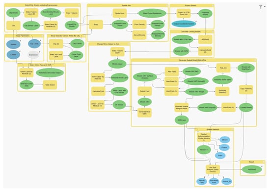
Figure A1.
Hot Street Model within ModelBuilder.
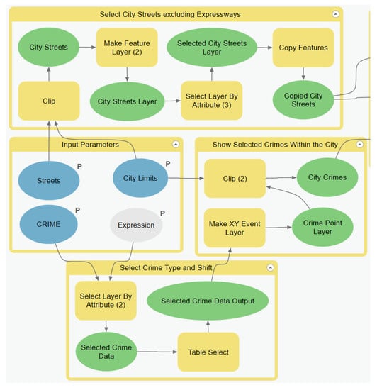
Figure A2.
First four sub-models.
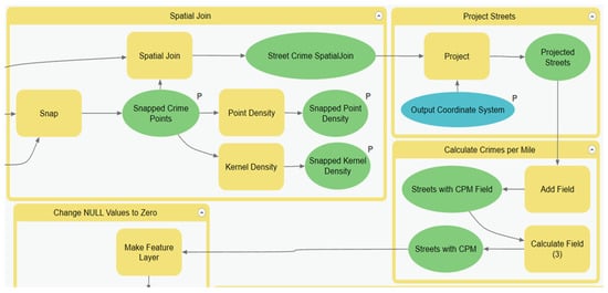
Figure A3.
Central model.
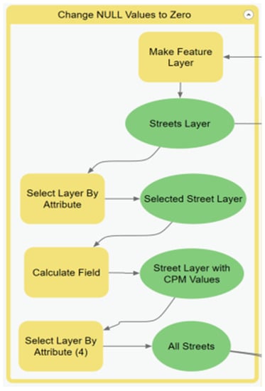
Figure A4.
Change Null Values to Zero sub-model.
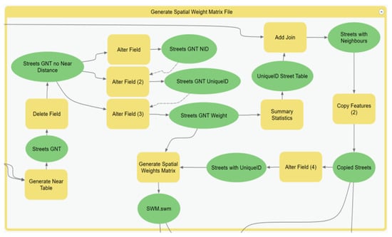
Figure A5.
Generate Spatial Weight Matrix sub-model.
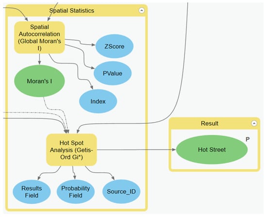
Figure A6.
Spatial Statistics sub-model.
References
- Brantingham, P.L.; Brantingham, P.J. Environment, Routine, and Situation: Toward a Pattern Theory of Crime. In Routine Activity and Rational Choice; Clark, R.V., Felson, M., Eds.; Transaction: Piscataway, NJ, USA, 1993; Volume 5, pp. 259–294. [Google Scholar]
- Scott, L.; Warmerdam, N. Extend crime analysis with ArcGIS spatial statistics tools. Arcuser Online 2005, 8, 2. [Google Scholar]
- Bruce, C.W.; Smith, S.C. Spatial Statistics in Crime Analysis: Using CrimeStatIII, 2nd ed.; National Institute of Justice: Washington, DC, USA, 2011; pp. 1–151.
- Santos, R.B. Crime Analysis with Crime Mapping, 4th ed.; SAGE: Thousand Oaks, CA, USA, 2016. [Google Scholar]
- Braga, A.; Papachristos, A.; Hureau, D. Hot spots policing effects on crime. Campbell Syst. Rev. 2012, 8, 1–96. [Google Scholar] [CrossRef]
- Braga, A.A. Problem-Oriented Policing and Crime Prevention, 2nd ed.; Criminal Justice Press: Monsey, NJ, USA, 2008. [Google Scholar]
- Eck, J.E. Preventing crime at places. In Evidence-Based Crime Prevention; Farrington, D.P., MacKenzie, D.L., Sherman, L.W., Welsh, B.C., Eds.; Routledge: New York, NY, USA, 2002. [Google Scholar]
- Grana, G.; Windell, J.O. Crime and Intelligence Analysis: An Integrated Real-Time Approach; CRC Press/Taylor & Francis Group: Boca Raton, FL, USA, 2017. [Google Scholar]
- National Research Council. Fairness and Effectiveness in Policing: The Evidence; Skogan, W., Frydl, K., Eds.; National Academies Press: Washington, DC, USA, 2004; p. 250. [Google Scholar]
- Weisburd, D.; Eck, J.E. What can police do to reduce crime, disorder, and fear? Ann. Am. Acad. Political Soc. Sci. 2004, 593, 42–65. [Google Scholar] [CrossRef]
- Weisburd, D.; Lum, C. The diffusion of computerized crime mapping in policing: Linking research and practice. Police Pract. Res. 2005, 6, 419–434. [Google Scholar] [CrossRef]
- Telep, C.W.; Weisburd, D. Policing. In What Works in Crime Prevention and Rehabilitation; Springer: New York, NY, USA, 2016; pp. 137–168. [Google Scholar]
- Andresen, M.A.; Malleson, N. Testing the Stability of Crime Patterns: Implications for Theory and Policy. J. Res. Crime Delinq. 2011, 48, 58–82. [Google Scholar] [CrossRef]
- Weisburd, D.; Groff, E.; Yang, S.-M. The Criminology of Place: Street Segments and Our Understanding of the Crime Problem; Oxford University Press: Oxford, UK; New York, NY, USA, 2012; ISBN 9780199928637. [Google Scholar]
- Weisburd, D. The Law of Crime Concentration and the Criminology of Place*. Criminology 2015, 53, 133–157. [Google Scholar] [CrossRef]
- Gwinn, S.L.; Bruce, C.W.; Hick, S.R.; Cooper, J.P. Exploring Crime Analysis: Readings on Essential Skills, 2nd ed.; International Association of Crime Analysts: Overland Park, KS, USA, 2008. [Google Scholar]
- O’Brien, D.T. The Action Is Everywhere, But Greater at More Localized Spatial Scales: Comparing Concentrations of Crime across Addresses, Streets, and Neighborhoods. J. Res. Crime Delinq. 2019, 56, 339–377. [Google Scholar] [CrossRef]
- Schnell, C.; Braga, A.A.; Piza, E.L. The influence of community areas, neighborhood clusters, and street segments on the spatial variability of violent crime in Chicago. J. Quant. Criminol. 2017, 33, 469–496. [Google Scholar] [CrossRef]
- Eck, J.; Chainey, S.; Cameron, J.; Wilson, R. Mapping Crime: Understanding Hotspots. USA: National Institute of Justice. Available online: http://www.ojp.usdoj (accessed on 4 November 2017).
- Trepanier, E. Identifying High Crime Areas Using Spatial Analysis. In Proceedings of the Thinking Matters Symposium, Portland, OR, USA, 24 May 2014; p. 2. [Google Scholar]
- National Institute of Justice. How to Identify Hot Spots and Read a Crime Map. 2010. Available online: http://nij.ojp.gov/topics/articles/how-identify-hot-spots-and-read-crime-map (accessed on 27 September 2019).
- Anselin, L. Local Indicators of Spatial Association-LISA. Geogr. Anal. 1995, 27, 93–115. [Google Scholar] [CrossRef]
- Brazil, N.; MacDonald, B.; Wilson, J.; Mitchell, I.; Ngo, L.; Windisch, R.; Qian, Y.; Schoonover, K.; Franke, R. A Spatial Analysis of Street-level Crime Trends in Los Angeles. In Proceedings of the Los Angeles Geospatial Summit, Los Angeles, CA, USA, 24 February 2017; pp. 1–52. [Google Scholar]
- Getis, A.; Ord, J.K. The Analysis of Spatial Association by Use of Distance Statistics. Geogr. Anal. 1992, 24, 189–206. [Google Scholar] [CrossRef]
- U.S Census Bureau. Available online: https://www.census.gov/quickfacts/fact/table (accessed on 27 September 2019).
- City of Atlanta. Police. Available online: https://www.atlantaga.gov/government/departments/police (accessed on 17 September 2019).
- Houston Police Department. Available online: https://www.houstontx.gov/police/chief/ (accessed on 27 September 2019).
- U.S Census Bureau. TIGER/Line Shapefiles. Available online: https://www.census.gov/geographies/mapping-files/time-series/geo/tiger-line-file.html (accessed on 23 August 2018).
- Police Department. Crime Data Downloads. Available online: http://www.atlantapd.org/i-want-to/crime-data-downloads (accessed on 27 January 2018).
- Houston Police Department. Monthly Crime Data by Street and Police Beat. Available online: https://www.houstontx.gov/police/cs/Monthly_Crime_Data_by_Street_and_Police_Beat.htm (accessed on 23 August 2018).
- Regional Commission. Atlanta City Limits. Available online: http://opendata.atlantaregional.com/datasets/coaplangis:atlanta-city-limits (accessed on 26 October 2017).
- OpenStreetMap Contributors. Planet Dump. Available online: www.openstreetmap.org (accessed on 1 August 2018).
- International Association of Crime Analysts. Identifying High Crime Areas. White Paper, 2013. Available online: https://iaca.net/white-papers/ (accessed on 30 October 2019).
- Openshaw, S. The Modifiable Areal Unit Problem; Geo Books: Norwich, UK, 1983; pp. 3–5. [Google Scholar]
- Silverman, B.W. Density Estimation for Statistics and Data Analysis; Springer: Boston, MA, USA, 1986; ISBN 9780412246203. [Google Scholar]
© 2019 by the authors. Licensee MDPI, Basel, Switzerland. This article is an open access article distributed under the terms and conditions of the Creative Commons Attribution (CC BY) license (http://creativecommons.org/licenses/by/4.0/).