Abstract
The paper proposes a method supported by MATLAB for detection and measurement of missing point regions (MPR) which may cause severe road information loss in mobile laser scanning (MLS) point clouds. First, the scan-angle thresholds are used to segment the road area for MPR detection. Second, the segmented part is mapped onto a binary image with a pixel size of ε through rasterization. Then, MPR featuring connected 1-pixels are identified and measured via image processing techniques. Finally, the parameters regarding MPR in the image space are reparametrized in relation to the vehicle path recorded in MLS data for a better understanding of MPR properties on the geodetic plane. Tests on two MLS datasets show that the output of the proposed approach can effectively detect and assess MPR in the dataset. The ε parameter exerts a substantial influence on the performance of the method, and it is recommended that its value should be optimized for accurate MPR detections.
1. Introduction
Mobile light detection and ranging (LiDAR) systems, also known as Mobile Mapping Systems (MMSs), are an emerging survey technology that enable quick and accurate depiction of real-world three-dimensional (3D) road environments in the form of dense point clouds. The LiDAR comprises the Global Navigation Satellite System (GNSS), Inertial Measurement Unit (IMU), and laser scanning system. Due to their realistic representation of real-life objects, mobile laser scanning (MLS) data provide an ideal virtual environment for various computerized estimations, in which dangerous and cumbersome field measurements, such as sight distance [1], can be avoided. Moreover, rich information, such as intensity, scan angle, and trajectory of the inspection vehicle, is included in MLS data, which aids the recognition and segmentation of different objects. Given these remarkable advantages, MLS data have received ever-increasing attention from transportation researchers over the past years [2].
Existing MLS data-based studies in road engineering can be generally categorized into three types: road-geometry feature extraction, road-surface condition assessment, and road-asset inventory [3,4,5]. Though the specific objective of each category is different, the general concept of using MLS data is similar: that is, to automatically extract certain road information whose measurement is costly, time-consuming, and labor-intensive in the real-world.
Although MLS data have great potential in this area, its quality may be susceptible to missing point regions (MPR) [6,7]. As shown in Figure 1, the beams emitted from the laser scanner may be obstructed by obstacles (either static or mobile) and thus creating MPR [6]. These missing regions may cause severe information loss and data gaps. For instance, if road lamps completely fall within an MPR, they cannot be detected by algorithms, which causes an adverse effect on the inventory accuracy of road features. When objects are partially inside the MPR, the missing point issue may also increase the difficulty of object detection and segmentation [7]. In some cases when the mobile obstacle is small or travels reversely in the direction of the measuring vehicle, the generated MPR may not cause substantial data gap (see the area marked in red in Figure 1).
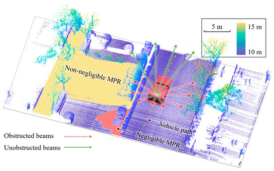
Figure 1.
Generation of MPR.
Whether an MPR causes non-negligible data gaps depends on its features (e.g., location, area, orientation). These features are associated with the obstacle attributes (e.g., position, dimension, speed of mobile vehicles in the traffic) at the time of capturing the points. Stationary obstructions are constantly fixed at their positions, so their impacts on MPR generation are relatively predictable. However, the traffic condition around the inspection vehicle at the data collection stage is hard to control, especially in busy cities, making the distribution of MPR along the road corridor difficult to predict. Therefore, it is meaningful to detect MPR in MLS data, which is a prerequisite for checking whether the road information loss (RIL) in the dataset is substantial.
Generally, detection of MPR on roads in MLS data involves two main steps: delineating the road area and segmenting MPR therein. Road area defines the search range for MPR while segmentation emphasizes MPR identification. In spite of the few studies that directly focus on detecting MPR, much attention in the literature was given to road-surface (or ground) extraction and road-boundary identification from MLS point clouds, both of which are related to road-area delineation.
Road-surface extraction is commonly a prerequisite for effective detection and classification of on-road objects in MLS data [3,4]. According to the review by Che et al. [3], existing methods of organizing MLS data for road-surface extraction can be generally categorized into three types: (1) rasterization, (2) 3D point, and (3) scanline methods.
Rasterization methods organize point clouds onto an image with a user-defined pixel size. The quality of the generated image is closely associated with the pixel size. Large pixel size may cause several points to fall within the same pixel and thus causing a substantial loss of details, while small pixel results in intensive computations. In the case where several points fall within the same pixel, the pixel-value is commonly represented by four different parameters: (a) the maximum elevation, (b) the minimum elevation, (c) the elevation difference, and (d) the number of points inside the pixel [8]. Assuming a planar segment as the road surface, rasterization methods use certain pixel-value difference as a threshold to segment surface from the generated image [9,10,11].
Compared with rasterization methods, the 3D point-based approaches can preserve the 3D nature of MLS point clouds. Nevertheless, due to the large volume of MLS data and the complexity of 3D calculations, 3D point-based methods are usually computationally intensive [3]. There exist various 3D point-based methods for ground filtering: (a) grid cell-based methods which partition points into grid cells and find points representing road surface in each cell [12,13,14], (b) triangulated irregular networks (TIN)-based methods which construct TIN from MLS points and use the features related to triangle elements to segment road surface [15,16], and (c) density-based approaches which calculate the number of neighboring points around each point within certain range and use a specific density value as a threshold to distinguish non-ground from ground points [17].
Both rasterization and 3D point-based methods partition MLS data into several vertical profiles. Unlike the preceding methods, the scanline methods first extract scanline profiles using the GPS time registered at the data collection stage. Then, in the scanning profile the road surface can be efficiently extracted using the scan angle and the height thresholds [18,19,20]. Some studies slice the cross-section profiles that are perpendicular to the vehicle path in MLS data and then extract the road surface using similar rules to the scanline methods [21,22].
However, extracting the road surface points may not contribute to accurate MPR detection. Figure 2 presents an example of a road surface extracted from highly noisy MLS data. As noted, due to the existence of MPR, it is a challenging task to recover the shape of the road corridor from the extracted road surface. In this case, the delineated road area would not be accurate.
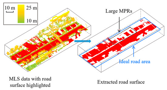
Figure 2.
Sample of extracted road surface in noisy MLS data.
Compared with ground filtering, more effort has been devoted in the literature to road boundary identification in MLS data [23,24,25,26,27,28]. However, the methods of organizing MLS data for identifying road boundaries are still similar to those of filtering ground points [3]. Besides, most existing methods for road boundary detection assume that road edges are higher than the road surface, which may fail in situations where road curbs are unavailable [12].
There are three main issues with respect to road area delineation using detected road boundaries in MLS data. First, as mentioned by Ma et al. [4], the existence of vehicle noises may degrade the performance of existing methods for road edge/curb identification. Second, the missing point regions in MLS data may cause substantial discontinuity in the identified road edges [6], which increases the difficulty in accurately delineating the road area. Third, some roadside features (e.g., road lamps) are located outside the road edges. In this case, only detecting MPR within the road boundaries cannot help determine whether such road features are missing in MLS data. Although the state-of-the-art methods may accurately extract road surface or detect road edges from MLS data, the severe MPR issue can make it challenging for those approaches to accurately delineate an ideal road area for MPR detection.
Despite the scarcity of studies that shed light on how to segment MPR from MLS data, some studies have recognized the MPR issue and proposed methods to automatically fill holes in the MLS point clouds. Hernández and Marcotegui [9] treated holes of an image as sets of pixels whose minima are not connected to the image border. Then, they removed all minima which are not connected to the border using the morphological reconstruction by erosion. The algorithm operated on the entire image and did not segment any specific MPR. In addition, the hole-filling algorithm may omit some large MPR according to their test results [9]. Doria and Radke [29] combined concepts from patch-based image inpainting and gradient–domain image editing to fill hole-structures in LiDAR data. However, their method was only tested for some typical scenes and did not involve detection of MPR.
Currently, a method for automatic detection and estimation of MPR in MLS data is still lacking. To fill the gap, this study aims to propose a post-processing pipeline for automated detection and measurement of MPR within the road area in MLS point cloud. Detection refers to the identification of MPR in the dataset, while measurement refers to quantitatively estimating the morphological features of MPR. Both processes are indispensable to assessing the extent of RIL in MLS data.
The following parts are structured as follows: Section 2 presents the material and method section which describes the MLS datasets used in this study and the MMS for collecting the data. Section 3 presents the algorithm description section which elaborates on the method developed for detecting MPR in MLS point cloud. Section 4 presents an application where the developed method was used to detect MPR in two MLS datasets. Finally, Section 5 presents our conclusions and the study limitations.
2. Materials and Methods
2.1. MLS Datasets
Two datasets containing scanning data of two different urban road sections shown in Figure 3a are used to test the method proposed for MPR detection in MLS point clouds. Both sections are situated in Qinhuai district, Nanjing, Jiangsu Province, P.R. China (N31°14′-N32°37′, E118°22′-E119°14′). The Hongwu road segment in Dataset 1 is 836.0 m long and 30.75 m wide with six lanes. The Zhongshan road segment in Dataset 2 is 562.0 m long and 27.70 m wide with six lanes. There are 10512319 and 8508372 points in Datasets 1 and 2, respectively. The point cloud resolution near the MLS trajectory is approximately 0.06 m in both datasets. The positioning accuracy of the two datasets is 1 cm + 1 ppm (horizontal) and 2 cm + 1 ppm (vertical). Figure 3b,c display different views of two road sections. There were many moving vehicles around the measuring car during the scanning of both road segments, so each dataset contains considerable MPR for the testing of the proposed method.
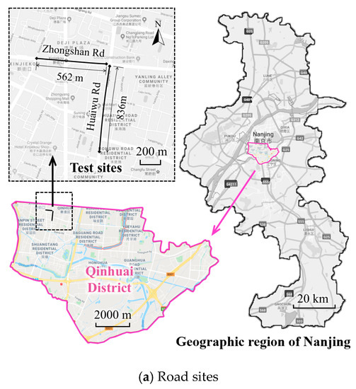
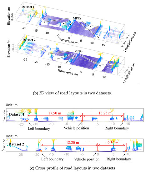
Figure 3.
Basic information regarding two road sections.
2.2. Mobile LiDAR System
The mobile LiDAR system used for collecting point cloud data is the Hi-Scan MMS from HI-TAGET [30]. The Hi-Scan MMS consists of three main parts: a SPAN® GNSS+IMU Combined System produced by Novatel [31], a single Z+F® laser scanner [32], and five high-quality digital cameras for capturing 360° views around the measuring vehicle. During the measuring process, the laser sensor emits high-frequency laser beams continuously. Every time a beam reaches an object, it returns to the laser mirror. Combining the time of flight data, the scan angle of laser beams, and the position information of the laser sensor recorded by the positioning system, the Hi-Scan can determine the 3D coordinates of each point in the coordinate system of the mapping frame. In this case, the
positioning information of points obtained through Hi-Scan MMS is in the World Geodetic System (WGS) 84 frame (E 120°, Gauss-Kruger Projection).
The mechanism of geo-referencing of Hi-Scan MMS is graphically shown in Figure 4a. As the scan angle and the scanning range of a point is determined, its position in the LiDAR scanner system can be obtained. Then, the position of in the coordinate system of the mapping frame is calculated as [4]:
where and are the positions of and the GNSS antenna in the mapping system, respectively; is the relative position of in the LiDAR scanner coordinate system; is the transformation information that aligns the IMU with the mapping frame where are roll, pitch, and yaw details of IMU in the mapping coordinate system; and is the transformation matrix that aligns the LiDAR scanner with the IMU. Other parameters involved in the geo-reference transformation and their values in the Hi-Scan MMS are summarized in Table 1. Figure 4b also presents different views of the Hi-Scan MMS component which help to understand the calibration parameters.
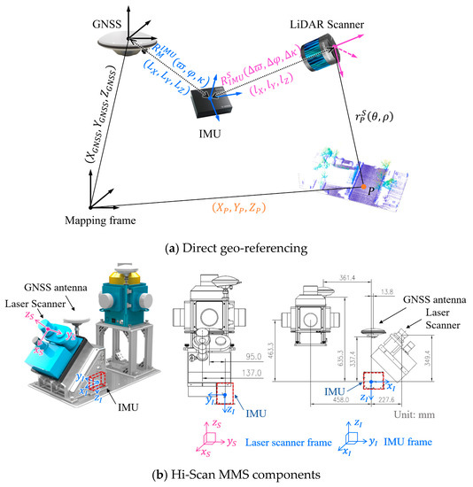
Figure 4.
Mechanism of direct geo-referencing.

Table 1.
Parameters in the geo-referencing transformation.
Detailed technical information regarding the Hi-Scan MMS is presented in Table 2. In this study, the highest scan frequency 200 Hz was selected to obtain denser point clouds. During the scanning process, the Hi-Scan MMS components were mounted 1.9 m high from the ground, and the inspection vehicle traveled along the same lane constantly at a speed less than 60 km/h.
Table 2.
Parameters regarding the Hi-Scan MMS.
3. Algorithm Description
3.1. Overview
The working flow of the developed method is graphically presented in Figure 5 and comprises four steps: (1) segmentation, (2) rasterization, (3) detection and measurement of MPR in the image and (4) parameterization of MPR on the geodetic plane. Specifically, in Step 1 using MLS data as input, the points within the road area are automatically extracted using the scan-angle thresholds. In Step 2, the obtained points are arranged onto the x-y plane in a grid manner to create a binary image. Then, the connected pixels labeled with 1 in the binary mask, which correspond to MPR in MLS data, are automatically detected and measured using a series of image processing algorithms in Step 3. Finally, in Step 4 the properties of MPR on the geodetic plane (e.g., location and area) are obtained via necessary parameterization and thereby the detection of MPR in LiDAR data is achieved. The entire method is implemented in the MATLAB environment.
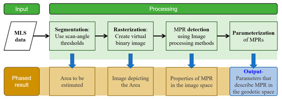
Figure 5.
Working flow of the proposed method.
3.2. Segmentation
Since this paper focuses on the estimation of MPR on roads, the points outside the road area are filtered out. In this study, the removal of points is realized using the scan-angle thresholds which have been successfully applied in several studies [18,19,20]. Figure 6a presents a cross-section view of the laser scan lines. The MLS point cloud is composed of numerous two-dimensional (2D) profiles that correspond to each rotation of the LiDAR scanner. Each point from a 2D profile (i.e., the scan plane in Figure 6a) has an angle value relative to the laser sensor. It is worth noting that Figure 6a is simply used for illustration as the scan plane of MMS is not necessarily parallel to the cross profile [4]. For instance, the angle between the scan plane (i.e., the plane in Figure 4b) of the Hi-Scan MMS and the cross profile (that is perpendicular to the forward direction) is 45° [30].
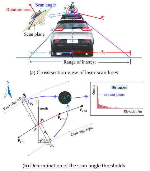
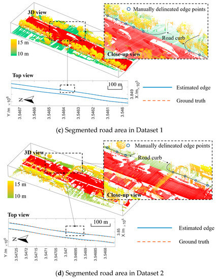
Figure 6.
Segmentation of point cloud.
The vertical offset of the laser scanner from the road surface is constant during the field survey. Therefore, there is a relatively stable geometrical relationship between the scan angle and the horizontal distance from the laser sensor to every point captured [19]. In the mobile LiDAR system, all sensors are aligned with the positioning system and linked through the time stamp [4], so each point recorded in the MLS dataset is relative to the inspection vehicle trajectory. Hence, in this study, and , which are the horizontal offsets from the vehicle path to the left and right road edges, respectively, are used to obtain the scan-angle thresholds. Because some road features are located outside the road edges, it is advisable to adjust and to extract different regions of interest (ROI) for MPR estimations.
The determination of the scan-angle thresholds was done manually in the literature [18,19,20], which is not flexible to address different ROI. Therefore, an algorithm for automated estimation of the scan-angle thresholds, illustrated graphically in Figure 6b, is developed in this phase. First, let and (, is the number of vehicle path points) be two consecutive points along vehicle trajectory which can be viewed as a good representation of the road axis [33]. The tangential vector at is . In this case, the azimuth of the vehicle path at is calculated as:
where and are plane coordinates of and , respectively, and is the horizontal distance between and . This distance is associated with the inspection vehicle speed and the selected output rate of the GNSS receiver during the data collection stage [34]. To achieve a smooth representation of the road alignment, especially on curved segments, this distance is recommended to be controlled as less than 5 m [33].
Second, calculate the plane coordinates of the respective points on the left and right road boundaries as follows:
where and are the plane coordinates of the left () and the right () boundary points at , respectively.
Third, as shown in Figure 6b, find neighbors within the radius of r around and separately in the MLS point cloud using the kd-tree algorithm [35], where, any point in the dataset whose horizontal distance from or is less than is obtained. In this study, is adopted as for and for . The empirical results regarding the influence of on the scan-angle threshold are presented in Appendix A. Then, for each boundary point, a histogram along the elevation of the points inside the circle is established with bin size empirically set as 0.05 m. The highest bin in the histogram normally corresponds to the surface points [36]. Hence, the points with elevation exceeding the right edge of the bin and containing the peak in the histogram are excluded. Subsequently, the scan-angle thresholds are determined as:
where () and () are the scan angle of the remaining points in the left and right circles, respectively. If , , otherwise and if , , otherwise . The variables and are the number of points in the respective ranges.
The algorithm starts from a random selection of a path point and then calculates and using Equations (6) and (7). If or falls inside an MPR, where the thresholds obtained are incorrect, once the algorithm detects that there is no point in either circle, a new path point will be selected to calculate the scan-angle thresholds. Using the proposed algorithm, the scan-angle thresholds can be determined without knowing the orientation of the rotation axis of the LiDAR scanner. Let be scan angle of each point in the MLS dataset. Depending on whether is an acute angle, there are two cases regarding the segmentation based on the scan-angle thresholds. Case 1: If , only the points with are retained while the other points are omitted. Case 2: If is a small acute angle, the points with and are retained.
As shown in Figure 6c,d, to validate the results of the segmentation, the points on the road edges in both Datasets 1 and 2 were manually selected. Continuous lines that connect the selected points on the two sides were viewed as the ground truth. The points along the left and right edges of the segmented ROI (points marked in red in Figure 6c,d) were also manually delineated and taken as the estimated boundaries. Then, these boundaries were compared with the ground truth. In Dataset 1, the algorithm produced desirable results as the estimated boundaries overlap substantially with the ground truth.
However, as marked with a rectangle in Figure 6d, the estimated boundaries in Dataset 2 show obvious deviation from the ground truth. The estimated boundaries are associated with the vehicle path. During the data collection, although the inspection vehicle is expected to strictly trace the lane centerline constantly, the surrounding vehicles may encroach into its travel lane and force it to shift transversely. This can explain why the estimated ROI boundaries did not overlap with the ground truth in Dataset 2 at some positions. The issue in Dataset 2 can be mitigated by slightly lengthening and , ensuring that the road area is included in the ROI.
3.3. Rasterization
With respect to the MPR measurement, the 2D parameters (e.g., area) can provide a clearer understanding of the MPR features in comparison with the 3D features. Moreover, implied by existing studies [25,26], analyzing MPR on the x-y plane helps reduce the dimension of the point cloud, making it more manageable and thus decreasing the computational time. Therefore, the MPR detection and measurement were performed on the horizontal plane in the study.
In Figure 6c or Figure 6d, it can be observed that there is an obvious contrast between an MPR and its adjoining regions. In this case, some well-established image processing algorithms can help identify MPR if the points are transformed into pixels. In addition, the removal of points with θ-value outside the angle range in the previous phase helps eliminate objects higher than the laser sensor. As such, objects like tree crown will not affect the accurate detection of MPR. Therefore, a rasterization method is applied to convert the point cloud data into a 2D binary image. Similar methods have been proved as effective for processing point cloud [37].
First, the remaining points are organized onto the x-y plane to create a 2D grid representation of the road area as follows:
where represent any point in and is a function for rounding a number to an integer. The and -values of the residual points are rounded to integral multiples of . The resolution of the generated model is closely associated with the grid size . Finer grids can result in a more accurate representation of the original point cloud. However, a small also causes disconnected pixels in an MPR, which may produce the adverse effects on the detection of MPR in the following steps. For simplicity, is used to represent the gridded point cloud data in the coordinate format.
Suppose a large bounding box fully encloses , as shown in Figure 7a. Let and be plane coordinates of the upper-left and lower-right corners, respectively. Let be the unit length. In this case, the horizontal and vertical distances from any point (gridded) to are both positive integers. Based on this feature, each 2D point in can be transformed into an element (or pixel) in a matrix (or image) as shown in Figure 7a. Taking for an illustration, the process of rasterization includes the following steps:
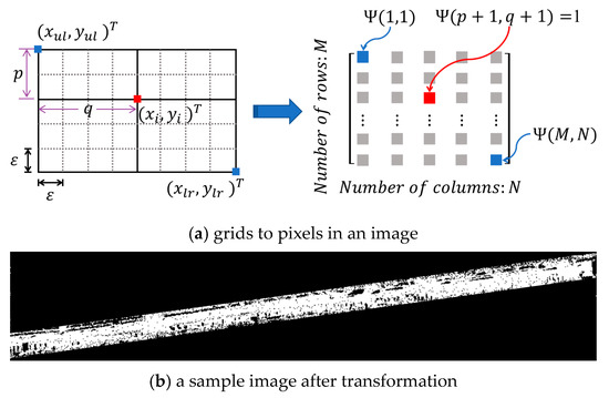
Figure 7.
The process of rasterization.
Step 1: Construct an matrix with all elements equal to zero, as follows:
where and are the number of rows and columns, respectively, and is the unit length.
Step 2: Calculate the vertical distance and the horizontal distance from to .
Step 3: Make the element in the )-th row and )-th column equal to 1, that is, .
A binary mask that corresponds with the gridded point cloud can be constructed by converting all points in . Figure 7b displays a sample image after the conversion. In this phase, the measurement of MPR in is equivalent to estimating the areas that feature connected pixels with 0-value within the road range in the binary image (i.e., ).
Usually, the inverted distance weighting (IDW) or the natural neighborhood interpolation (NNI) methods are used to rasterize the MLS points. However, when the pixel (grid) size is small, the IDW and NNI rasterization methods are computationally intensive. On the contrary, although the rasterization process in this study may cause a small shift of the MLS points, it can generate the binary image more efficiently without compromising the accuracy of the MPR detection. The comparison results of the rasterization methods on processing time and accuracy are presented in Appendix B.
3.4. Measurement of MPR in the Image
After years of development, the image processing algorithms for automatically detecting connected pixels with 1-value in a binary image are well established, which helps to quickly identify the MPR. The pixel-based complement can reverse the pixel value (i.e., 0 to 1 or 1 to 0) in the binary map, in which case the MPR is converted to connected pixels with 1-value. Nevertheless, the areas outside the road in the image also contains pixels with 1-value after the complementation, which causes adverse effects on the accurate detection of the MPR. Therefore, several image processing techniques are sequentially applied to address this issue and thereby improving the accuracy of MPR estimation. Figure 8 shows the general procedure for eliminating the impact of the areas outside the road on MPR detection. The image processing functions entailed are also presented.
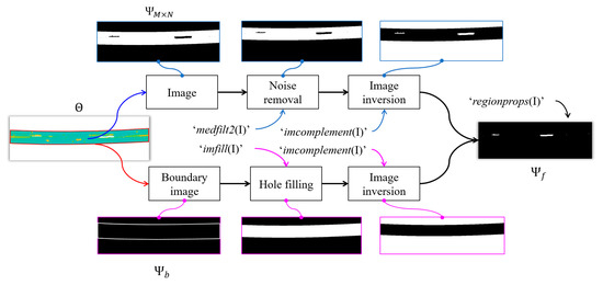
Figure 8.
Sequential application of image processing methods.
Let be the matrix representing the boundary image illustrated in Figure 8. Then the procedure for obtaining the final image for MPR detection can be expressed as:
where conducts the median filtering of the image to remove potential noises (isolated pixels with 1-value), outputs the pixel-based complement of the inputted image, and fills the areas enclosed by continuous pixels with 1-value in an image. These functions are all mature algorithms embedded in MATLAB [38].
Because has been obtained in the previous stage, the gap is for the purpose of obtaining . is transformed from points bounding , so the kernel is to calculate the coordinates of points in boundaries of . As previously described in the segmentation part, and , which are used to calculate the scan-angle thresholds from the MLS data, separately indicate the boundary positions on the two sides. Therefore, the boundary points can be derived from vehicle path coordinates using Equations (4) and (5). The function works only when it detects fully connected and loop-like pixels with 1-value, as shown in Figure 8. Nonetheless, the interval of boundary points is related to the gap of the vehicle path points, which may be larger than , causing disconnection between pixels that represent the boundary points, thus disabling the function. To resolve this issue, natural cubic splines (NCS) were used to fit the boundary points and then partitioned them into narrower and more uniform points.
Given a set of knots, the function is available to construct an NCS [39], yet an algorithm for adding knots on NCS is lacking in MATLAB. The concept of the algorithm for uniformly dividing the NCS is illustrated in Figure 9a, in which and are three consecutive points (i.e., knots or nodes) that constitute the NCS. The curves between each two adjacent knots are in the piecewise polynomial form. To illustrate, consider the curve between and for example. The coordinates of each point on the curve passing through and are given by:
where and are polynomial coefficients, is the square root of the chord length [40], and is given by:
where is the Euclidean distance between .
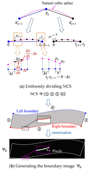
Figure 9.
Adding points on an NCS.
Equations (13)–(15) indicate that each curve between two sequential knots maps onto a curve along the -axis. In order to obtain the curve length between and , the -axis is discretized into points with a small interval of , where is computed as:
where is the length of line segment on NCS which corresponds to on the -axis, is the aliquot part of , and (which corresponds to the remainder part of on the -axis) is the Euclidean distance between and .
To obtain dense points with a gap of on NCS, the algorithm originates at and proceeds along the NCS at a pace of . Once the cumulative length reaches , it is reset to zero and the point is recorded and the algorithm continues until the end point () is reached. If cannot be exactly divided by , the remainder () will affect point acquisition in the curve between and as shown in Figure 9a, guaranteeing that the new knots are evenly distributed along the whole curve. The code of the algorithm is presented in Appendix B.
As shown in Figure 9b, there are four boundary lines including left (④) and right (②) boundaries as well as two line-segments (① and ③) that connect the vertices of the two boundaries for a given road section. NCS were separately applied to add points on each boundary line. Then, the that contains 1-value pixels corresponding with the boundary points can then be generated through the previously described rasterization method. Note that the size of should be consistent with in this step.
If is not exactly bounded by , the function is recommended to remove potential isolated 1-pixels in before MPR assessment. As seen from Figure 8, only the missing point regions remain after the processing, which aids the estimation of the MPR in the final image. Then, an efficient function , implemented in MATLAB [38], is used to quantify the properties of the regions formed by the connected 1-pixels (i.e., MPR). Considering the potential impacts on RIL, five properties illustrated in Figure 10 are empirically chosen for MPR assessment in this study: (1) in the image coordinate system , the centroid denotes the position of MPR, (2) the major axis length and (3) the minor axis lengths of the bounding ellipse approximately reflect the shape of the MPR, (4) the angle between the major axis of the bounding ellipse and the -axis shows the orientation of MPR, and (5) the area indicates the size of MPR. These parameters can quantitatively describe the missing point regions and help understand their features in the dataset.
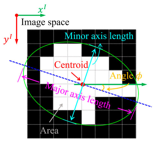
Figure 10.
Properties of MPR in the image.
The preceding properties may provide a comprehensive understanding of the MPR, but most of them are measured in pixels. To boost their value in real-world cases, further parametrization on the geodetic plane is necessary, as described next.
3.5. Parameterization of MPR on Geodetic Plane
At this stage, a coordinate transformation is first conducted to convert pixel positions in the binary image to 2D coordinates on the geodetic plane as follows:
Subsequently, each MPR feature measured in the binary image is transformed into a parameter in the geo-referenced MLS data. Table 3 shows the MPR parameters in two different spaces. Methods for mathematically transforming each feature are also shown.
Table 3.
MPR Parameters in two different spaces.
Because represents the pixel size in the real world, the area, and the minor and major axes lengths can be simply scaled by multiplying them by or as shown in Table 3. As previously mentioned, MPR detection is a prerequisite for estimating RIL on roads. In the civil engineering field, most road information, such as geometric parameters, road lamps, and traffic signs is registered in relation to the road axis (e.g., indexed with station). In this case, linking MPR features with the road axis is beneficial for understanding their effects on road-attribute extraction in future research. Therefore, the angle and centroid are re-parameterized in relation to the road axis.
Nonetheless, accurate extraction of the road centerline from MLS data is a challenging task and may depend on the quality of point cloud data [18], which is not the focus of this work. Hence, the vehicle trajectory that traces the centerline is used in this study to represent the road axis.
3.5.1. Offset from Vehicle Trajectory
Figure 11 illustrates the MPR corresponding to Figure 10 in the point cloud form. The offset from the vehicle trajectory is calculated by obtaining the distance between A and B in Figure 11, where A is the centroid of the MPR and B is the vehicle track point which makes the line segment AB perpendicular to the vehicle trajectory. The coordinate of A is available via Equation (17), so the kernel of calculating the offset from the vehicle trajectory aims at finding B.
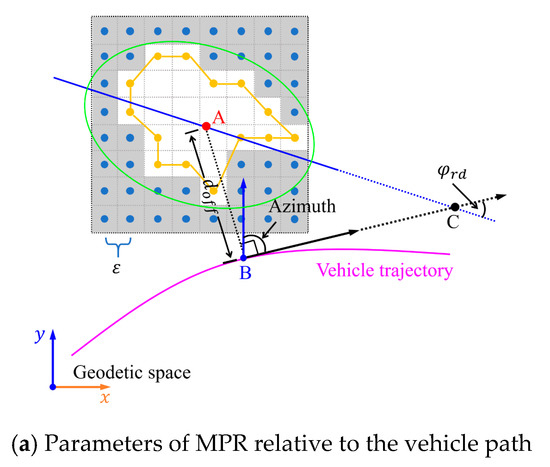
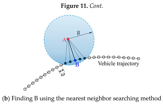
Figure 11.
Calculation of offset from the vehicle trajectory.
The interval of the path points can be narrowed to using the algorithm in Figure 9, making the discretized points a good representation of the continuous vehicle trajectory. Under this circumstance, B can be approximated using a nearest neighbor searching method. Specifically, as shown in Figure 11b, a virtual circle centered at A is established using the function in MATLAB to find neighbors around A within a radius of . The point therein with the smallest distance to A is determined as B.
As the interval of dense path points is known, the distance from the starting point (of vehicle path) to B along the vehicle trajectory can be calculated, where the centroid is located as (). To make it easier for the users to understand which side of the vehicle trajectory the MPR is situated, is set as negative for the right-side MPR, and positive for the left-side MPR.
3.5.2. Angle between Major Axis and Vehicle Trajectory
With the position of B determined, the angular relationship between the major axis of the ellipse enclosing the MPR and the vehicle path can be estimated. Let C be the point where the major axis intersects with the tangential direction of the vehicle trajectory at B. Then, the angle of concern is between the vectors and (Figure 11a).
In the binary map, the angle between the major axis and the axis (see Figure 10) is negative when the axis demands clockwise rotation around the centroid to arrive at the major axis, otherwise it is positive. The criterion remains unchanged in the computation of except that the axis is substituted with the tangential vector . Under this condition, there exist four cases with respect to the calculation of (see Figure 12a–d):
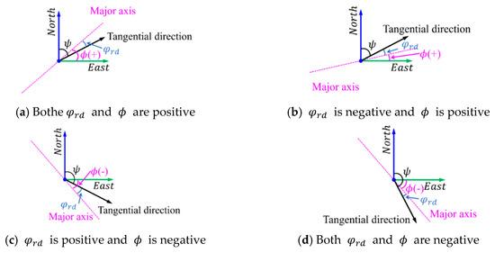
Figure 12.
Calculation of .
Case A (Figure 12a): Both and are positive, and is given by:
where is the azimuth of the horizontal vehicle path at B.
Case B (Figure 12b): is negative and is positive, and is given by:
Case C (Figure 12c): is positive and is negative, and is given by:
Case D (Figure 12d): Both and are negative, and is given by:
Clearly, according to Equations (18) to (21), equals in all cases.
4. Application
In this section, the developed method was applied to detect the MPR in the two MLS datasets previously mentioned. The variables involved in the method were specified as shown in Table 4. In this case, was set as 0.10 m for accurate detection of the MPR. The effect of on MPR measurement is discussed later.
Table 4.
Values of the variables adopted in the method.
4.1. MPR Detection Test
In addition to the measurement of the MPR, connected 1-pixels which represent the MPR in the binary image were converted to points in the Cartesian coordinates using Equation (17). In this way, the MPR identified by the algorithm can be visualized in the point cloud environment as displayed in Figure 13.
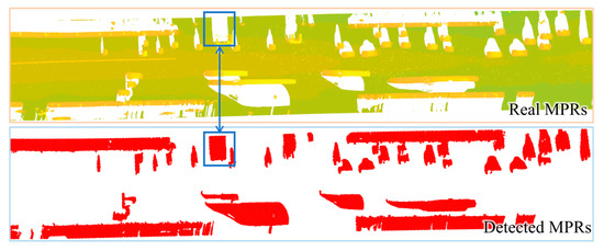
Figure 13.
Comparison of real and detected MPR in the point cloud environment (ε = 0.1 m).
In this case, it is viable to visually examine the false positives and negatives that are detected by the method. Different -values (from 0.04 to 0.26 with an interval of 0.02) were separately applied to produce different estimations of the MPR. Then, using different values, stepwise comparisons between real and detected MPR were manually made for each dataset (Figure 13), finding that every MPR was correctly identified and located when . Regarding other -values, although some small MPR were neglected by the algorithm, all the identified ones were correct with respect to their positions. These findings demonstrate that the proposed method is effective for MPR detection. For a better performance of the algorithm, was used in the subsequent assessment of MPR.
4.2. MPR Mesurement in Two Datasets
The numerical parameters that describe MPR in each MLS dataset can be obtained via the proposed method. To make it easier for the users to understand MPR in the given MLS data, five parameters (area, offset, major axis length, minor axis length, and angle) were all indexed to the distance () from the starting point, so that these parameters can be developed into graphics like Figure 14 and Figure 15.
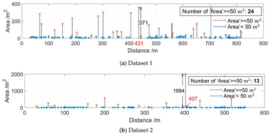
Figure 14.
Stem diagrams regarding the MPR area.
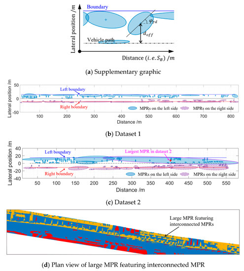
Figure 15.
Visualization of MPR properties.
The generated areas of MPR along each road section are shown in Figure 14, where the height of every stem in each figure represents the scale of the MPR area. Figure 14 helps understand the positions along the road where it suffers large MPR that may cause severe RIL. For instance, the positions where the MPR area exceeds 50 are highlighted in both Figure 14a,b. There are 24 MPR whose area is larger than 50 in Dataset 1 while only 13 counterparts are observed in Dataset 2. The number of large MPR in Dataset 1 outstrip that in Dataset 2. However, the maximum area of MPR in Dataset 2 is 1994 at 407 , which is far larger than that of 371 at 431 in Dataset 1.
A preliminary knowledge of MPR can be learned from Figure 14, yet it only contains area information. Hence, a supplementary graphic illustrated in Figure 15a is used to provide a better understanding of the MPR results. Each MPR inside the ROI is represented by its bounding ellipse. The centroid is located at () and the angle between the major axis of the ellipse and the distance axis is . The boundary lines that delineate the borders of ROI are also shown.
Features like size, orientation, and distribution of MPR along the road can be directly appreciated from Figure 15b,c, albeit no numerical data were provided. The ellipses on the right and left sides of the vehicle trajectory are distinctly marked, so that it is possible for the users to compare which side may suffer MPR more. For example, the MPR on the left side of the vehicle path are larger than those on the right in Figure 15c, implying that the RIL issue on the left side in Dataset 2 may be more severe. Figure 15c also demonstrates the existence of the extremely large MPR at 407 m (see Figure 14b). The immense MPR in Dataset 2 can be understood by referring to its shape in the point cloud environment, as illustrated in Figure 15d. For the case when the traffic was heavy at the time of the laser scanning, small MPR may connect to form a larger MPR.
4.3. Sensitivity Analysis
The variable plays a crucial role in establishing the binary map and is closely associated with the image resolution, which may substantially affect accurate measurement of MPR. Therefore, the effect of on MPR measurement was evaluated in this study. Different -values from 0.04 to 0.26 with an interval of 0.02 were used to generate different MPR estimations. As previously mentioned, the proposed method achieved satisfactory performance on detecting MPR in MLS data when , so the MPR estimations generated using other -values were all compared with the results of this value through one-way analysis of variance (ANOVA) tests. Specifically, for each -value, the difference between the five estimated MPR features and those of were separately examined. The test results are summarized in Table 5. The P-value lower than 0.05 indicates a statistically significant difference between two samples at the 95% confidence level. In this case, P < 0.05 means the results concerning a specific parameter measured are unreliable.
Table 5.
Statistical analysis of MPR measurements a.
It can be drawn from Table 5 that exerts a significant effect on the MPR detection and measurement. As shown in the second column of Table 5, either an increase or a decrease in the -value may reduce the number of identified MPR in both datasets. As the -value increases, the resolution of the binary image decreases, in which case some details in the original LiDAR data may be omitted due to the rough rasterization and thereby causing neglect of some small MPR. On the contrary, a smaller can better represent the original data but may also lead to disconnection between pixels inside the MPR. A main drawback to rasterization lies in the fact that the point cloud resolution is highly variable with MLS data and greatly further degrades from the vehicle path. The operation in the method would exclude isolated pixels. Hence, the MPR in which the pixels are not fully connected cannot be correctly detected. Therefore, the number of MPR detected by the method can serve as an indicator that shows whether the MPR are adequately identified.
There is no fixed pattern regarding the influence of on the reliability of the measured parameters. The five parameters showed different susceptibilities to the change in and the ANOVA results varied between the datasets. However, it can be concluded that the MPR estimations become unreliable when the deviation from of 0.10 reached a certain extent. These findings indicate that there exists an optimal -value with respect to the MPR detection and measurement using the developed approach. Therefore, for a more accurate MPR measurement, it is recommended to adjust the -values using partial data extracted from the entire MLS dataset to determine the optimal -value before the final MPR estimations.
5. Concluding Remarks
This paper has proposed a solution for automated detection and measurement of road’s missing point regions in mobile laser scanning data. The effectiveness of the method was demonstrated using tests on two MLS datasets. The results show that the method can identify and locate MPR correctly within ROI. In addition, five properties of MPR were quantitatively measured and developed into graphics using the proposed approach, which helps better understand morphological features of MPR and paves the way for future investigation into how MPR features are related to the RIL issue. The ANOVA tests suggest that there is an optimal ε-value regarding detection of MPR in MLS data using the proposed approach.
Some issues remain to be addressed in future research. The developed approach relies on vehicle trajectory data. In this study, the measuring vehicle traces the road axis carefully by remaining in the same lane during data collection, but there is a possibility that the vehicle must shift to another lane for turning or passing maneuvers. In these cases, the extracted ROI may not be exactly the road area. Further research to estimate the adverse effect of using vehicle path as a substitute for the road axis is needed. Also, the proposed method extracted the road area from the MLS point cloud using the scan-angle thresholds, while in some MMS, more than one laser scanners are used (e.g., Trimble MX-9), which may degrade the accuracy of the extracted road area. A more robust method for delineating the road area in MLS data for MPR detections is expected to be developed in the future.
As previously mentioned, the detection of MPR in MLS data is a first step for investigating the relationship between MPR properties and RIL. Although the RIL issue can be estimated by determining whether important road features fall inside MPR in some contexts, when the road furniture data are missing or road information concerned is a parameter (e.g., road curve radius), such an estimation is impracticable. Therefore, it is meaningful to find the specific parameters that can serve as effective indicators of RIL in future research. This would help to directly determine from MPR parameters whether RIL is significant.
Author Contributions
Conceptualization, Yang Ma; Methodology, Yang Ma, Yubing Zheng; Validation, Yang Ma, Yubing Zheng; Formal Analysis, Yang Ma, Yubing Zheng, Said Easa; Writing-Original Draft Preparation, Yang Ma, Yubing Zheng, Said Easa; Writing-Review & Editing, Said Easa, Mingyu Hou; Visualization, Yang Ma; Funding Acquisition, Yang Ma, Jianchuan Cheng; Supervision: Jianchuan Cheng.
Funding
This research was jointly supported by National Natural Science Foundation of China (grant number: 51478115), Postgraduate Research & Practice Innovation Program of Jiangsu Province (grant number: KYCX19_0107), and Scientific Research Foundation of Graduate School of Southeast University.
Acknowledgments
The authors would like to express special thanks to Wenquan Han from Nanjing Institute of Surveying, Mapping & Geotechnical Investigation, Corp. Ltd. for providing data used in this study and the anonymous reviewers for their valuable and most helpful comments.
Conflicts of Interest
The authors declare no conflict of interest. The funders had no role in the design of the study; in the collection, analyses, or interpretation of data; in the writing of the manuscript, or in the decision to publish the results.
Notations
The following notations are used in this paper:
| Left boundary point | |
| Right boundary point | |
| Offsets between the GNSS origin and the IMU origin | |
| , | Three consecutive nodes that constitute the NCS |
| M | Number of rows of the matrix |
| Number of columns of the matrix | |
| , | Two consecutive points along the vehicle trajectory |
| Radius that helps determine | |
| Transformation matrix that aligns the LiDAR scanner with the IMU | |
| Transformation information that aligns the IMU with the mapping | |
| Distance that is measured along the vehicle path from the starting point | |
| Polynomial coefficients | |
| Horizontal offset from the vehicle path to the left road edge | |
| Horizontal offset from the vehicle path to the right road edge | |
| Offset from the vehicle path to the centroid of MPR | |
| Function that outputs the pixel-based complement of the inputted image | |
| Function for filling the areas enclosed by continuous 1-value pixels in an image | |
| Offsets between the IMU origin and the LiDAR scanner origin | |
| Function for the median filtering of the image to remove potential noises | |
| Number of vehicle path points | |
| Vertical distance from to | |
| Remainder part of on the -axis | |
| Horizontal distance from to | |
| Radius around or | |
| Function for rounding a number to an integer | |
| Relative position of in the LiDAR scanner coordinate system frame | |
| Curve length between | |
| Square root of the chord length | |
| Any point in | |
| Image space | |
| Plane coordinates of the left () boundary points at | |
| Plane coordinates of the right () boundary points at | |
| Position of GNSS antenna in the mapping system | |
| Plane coordinates of | |
| Plane coordinates of | |
| Plane coordinates of the lower-right corner of the bounding box enclosing | |
| Coordinates of each point on the curve passing through and | |
| Position of in the mapping system | |
| Plane coordinates of the upper-left corner of the bounding box enclosing | |
| Length of line segment on NCS which corresponds to on the -axis | |
| Interval along the -axis | |
| Bore sight angles that align the LiDAR scanner with the IMU | |
| Gridded point cloud data in the coordinate format | |
| Matrix representing boundary image | |
| Matrix representing the final image for the MPR detection | |
| Gridded point cloud data in the matrix format | |
| Scan angle of the left boundary point | |
| Scan angle of the remaining points in the left circle | |
| Scan angle of the right boundary point | |
| Scan angle of the remaining points in the right circles | |
| Pixel size | |
| Number in the range for | |
| Number in the range for | |
| Scan angle of each point in the MLS dataset | |
| Variables in the calculation of | |
| Yaw angle of IMU in the mapping coordinate system | |
| Roll angle of IMU in the mapping coordinate system | |
| Remainder on the NCS between and | |
| Scanning range in the LiDAR scanner system | |
| Pitch angle of IMU in the mapping coordinate system | |
| Angle between major axis of bounding ellipse and axis | |
| Angle between major axis of bounding ellipse and axis in the image space | |
| Azimuth of the horizontal vehicle path at B | |
| Azimuth of the horizontal vehicle path at | |
| Gap between points on an NCS |
Appendix A. Effect of on Scan-Angle Thresholds
In each dataset, two positions (that do not suffer MPR issues) are selected to investigate the influence of on the scan-angle thresholds. For each position, the distance from the path point (along the normal direction) is and the radius of the circle is . In the tests, five -values (2.0, 4.0, 6.0, 8.0 10.0 m) are used. For each -value, five -values are applied to determine the scan-angle thresholds. The accurate scan angle is manually determined for each -value. Then, the absolute error (ASE = ) is used to measure the difference between the accurate scan angle and that determined by the algorithm. The results are summarized Table A1 and Table A2.
Table A1.
Test results of Dataset 1.
Table A1.
Test results of Dataset 1.
| (m) a | Absolute Error, ASE (°) | |||||
|---|---|---|---|---|---|---|
| Position 1 | 2.0 | 0.53 | 0.46 | - b | - | - |
| 4.0 | 0.15 | 0.36 | 0.35 | 0.50 | - | |
| 6.0 | 0.27 | 0.17 | 0.20 | 0.37 | - | |
| 8.0 | 0.35 | <0.10 | <0.10 | 0.19 | 0.24 | |
| 10.0 | 0.62 | <0.10 | 0.16 | 0.27 | 0.38 | |
| Position 2 | −2.0 | 0.45 | 0.36 | - | - | - |
| −4.0 | 0.23 | 0.24 | 0.56 | 0.57 | - | |
| −6.0 | 0.26 | 0.11 | 0.25 | 0.33 | 0.43 | |
| −8.0 | 0.24 | 0.15 | <0.10 | 0.36 | 0.27 | |
| −10.0 | 0.22 | 0.17 | <0.10 | 0.13 | 0.26 | |
a A negative value of d means the point is on the left, a positive value means the point is on the right. b A dash means there is no points in the circle.
Table A2.
Test results of Dataset 2.
Table A2.
Test results of Dataset 2.
| (m) a | Absolute Error, ASE (°) | |||||
|---|---|---|---|---|---|---|
| Position 1 | 2.0 | 0.23 | 0.15 | - b | - | - |
| 4.0 | 0.32 | 0.12 | 0.17 | 0.23 | - | |
| 6.0 | 0.22 | 0.15 | 0.23 | 0.22 | 0.28 | |
| 8.0 | 0.25 | 0.18 | 0.14 | 0.21 | 0.25 | |
| 10.0 | 0.12 | <0.10 | <0.10 | 0.10 | 0.13 | |
| Position 2 | −2.0 | 0.36 | 0.23 | 0.13 | - | - |
| −4.0 | 0.25 | 0.14 | 0.30 | 0.55 | - | |
| −6.0 | 0.38 | 0.14 | 0.11 | 0.16 | 0.22 | |
| −8.0 | 0.33 | 0.20 | 0.11 | 0.33 | 0.37 | |
| −10.0 | 0.34 | <0.10 | 0.27 | 0.31 | 0.29 | |
a A negative value of d means the point is on the left, a positive value means the point is on the right. b A dash means there is no points in the circle.
Appendix B. Comparison of Rasterization Methods
The inverse distance weighting (IDW) is a type of deterministic method for multivariate interpolation with a known scattered set of points [41]. The assigned values to the unknown points are calculated with a weighted average of the values available at the known points. In this case, the horizontal distance between each known point to the unknown point is used to calculate the weight. Figure A1 illustrates the concept of the IDW method. The rasterization process using the IDW method involves the following steps:
Step 1: Create many cells where each cell center corresponds to the pixel position in the final image. The cell size corresponds to the pixel size.
Step 2: Find the LiDAR points inside each cell using a nearest neighbor searching method (e.g., kd-tree searcher)
Step 3: Select a cell. If there is no point in the cell, the height value of the cell center is void, otherwise, go to Step 4
Step 4: Calculate the height of the cell center as follows
where is the distance from each LiDAR point in the cell to the cell center, is the calculated weight of each point, is the coordinate of the cell center, and are the coordinates of LiDAR points in the cell. Note that is adopted as 1.
Step 5: if is void, the pixel value is 0, otherwise the pixel value is 1.
Step 6: If all cells are calculated, the process is terminated. Otherwise, go to Step 3.
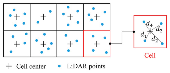
Figure A1.
Illustration of the IDW method.
The natural neighborhood interpolation (NNI) is another well-established method that can be invoked using the ‘griddata (.)’ function in MATLAB. It has been widely applied in 2D or 3D interpolation with a large set of unordered points [42]. However, the ‘griddata (.)’ function is inappropriate for direct application in this case because it may arbitrarily fill holes (i.e., MPR) in the MLS dataset [43]. To perform the rasterization without filling MPR, the rasterization process with the NNI method is similar to that using the IDW approach, except that the height in Step 4 is calculated with the ‘griddata (.)’ function instead of the IDW method.
Three rasterization methods are separately applied to generate the binary image. The processing time of different methods are summarized in Table A3. It can be observed from Table A3 that the simple method used in the study outperforms the other two methods with respect to computational efficiency for both MLS datasets. The MPR detection results in the two MLS datasets, using different pixel size, are shown in Figure A2. The horizontal axis in each figure refers to the distance to the starting point along the vehicle path, while the vertical axis represents different MPR features. From Figure A2a,b, it can be concluded that the difference between the rasterization method employed in the study and the other two methods is negligible because most points overlapped in the figures. Accordingly, it is advisable to use the simple method for rasterization of this study when the pixel size is relatively small (<0.3 m). However, it is not recommended to use this simple method when the pixel size is large because the operation may cause a large shift of points and thereby adversely affect the accuracy.
Table A3.
Processing time of different rasterization methods (a) Dataset 1 (2) Dataset 2.
Table A3.
Processing time of different rasterization methods (a) Dataset 1 (2) Dataset 2.
| Pixel (cell) Size (m) | Processing Time (s) | ||
|---|---|---|---|
| IDW | NNI | Method of This Study | |
| (a) Dataset 1 | |||
| 0.1 | 89.42 | 69.43 | 0.27 |
| 0.2 | 27.14 | 20.98 | 0.23 |
| 0.3 | 15.17 | 14.58 | 0.22 |
| (b) Dataset 2 | |||
| 0.1 | 54.71 | 27.98 | 0.24 |
| 0.2 | 17.77 | 15.56 | 0.19 |
| 0.3 | 15.17 | 13.58 | 0.18 |
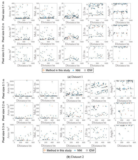
Figure A2.
MPR detection results using different rasterization methods.
Appendix C. MATLAB Source Code for Adding Uniformly Distributed Points on NCS
The code uses MATLAB syntax. The content following ‘%’ in the same line is annotation. ncs is a ‘struct’ type data output by . The symbol ‘.’ following ncs allows access to elements in ncs: ncs.pieces stores the number of line segments connecting two original sequential knots, ncs.breaks stores the cumulative -value along the spline, ncs.coefs stores the coefficients of piecewise polynomials. Details about MATLAB syntax can be found in the MATLAB official website [39]. The testing results generated by the algorithm are presented in Figure A3.
| Algorithm A1. Adding Uniformly Distributed Points on NCS |
| function points = uniformKnots (ncs,delta_t,w) |
| % ncs refers to the output of cscvn(.) |
| % delta_t (∆t) is a user-defined value (<=0.01) |
| % the output of uniformKnots(.) is denser points on NCS in the coordinate format |
| points = []; |
| d_res = 0; |
| for i=1:1:ncs.pieces |
| T = ncs.breaks(i+1) - ncs.breaks(i); |
| % T is the chord length |
| x = ppmak ([0 T],ncs.coefs(2*i-1,:)); |
| y = ppmak ([0 T],ncs.coefs(2*i,:)); |
| t = 0:delta_t:T; |
| p1 = [ppval(x,t(end)) ppval(y,t(end))]; |
| p2 = [ppval(x,T) ppval(y,T)]; |
| % p1 and p2 are last two points with gap less than delta_t |
| g = @(p) ncs.coefs(2*i-1,1)*3*p.^2 + ncs.coefs(2*i-1,2)*2*p + ... |
| ncs.coefs(2*i-1,3); |
| f = @(p) ncs.coefs(2*i,1)*3*p.^2 + ncs.coefs(2*i,2)*2*p + ... |
| ncs.coefs(2*i,3); |
| s = sqrt(f(t).^2 + g(t).^2) * delta_t; |
| num = length(t)-1; |
| lengthOfNcs = sum(s(1:end-1)) + norm(p1-p2); |
| % lengthOfNcs is s in Figure 9 |
| remOft = rem(lengthOfNcs + d_res,w); |
| % remOft is τ in Figure 9 |
| delta_d = 0; |
| for j = 1:1:num |
| delta_d = delta_d + s(j); |
| indicator = sign(delta_d - (w-d_res)); |
| lengthOfNcs = lengthOfNcs - s(j); |
| if indicator >= 0 |
| points = [points;ppval(x,t(j+1)) ppval(y,t(j+1))]; |
| delta_d = 0; |
| d_res = 0; |
| else |
| continue; |
| end |
| if lengthOfNcs <= remOft |
| d_res = lengthOfNcs; |
| break; |
| end |
| end |
| end |
| end |
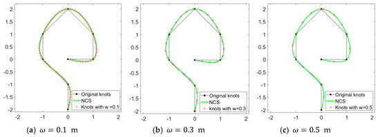
Figure A3.
Application of the algorithm for adding points on NCS.
References
- Ma, Y.; Zheng, Y.; Cheng, J.; Zhang, Y.; Han, W. A Convolutional Neural Network Method to Improve Efficiency and Visualization in Modeling Driver’s Visual Field on Roads Using MLS Data. Transp. Res. Part C Emerg. Technol. 2019, 106, 317–344. [Google Scholar] [CrossRef]
- National Cooperative Highway Research Program 748 Report: Guidelines for the Use of Mobile LiDAR in Transportation. Available online: http://onlinepubs.trb.org/onlinepubs/nchrp/nchrp_rpt_748.pdf (accessed on 4 October 2018).
- Che, E.; Jung, J.; Olsen, M. Object Recognition, Segmentation, and Classification of Mobile Laser Scanning Point Clouds: A State-of-the-Art Review. Sensors 2019, 19, 810. [Google Scholar] [CrossRef] [PubMed]
- Ma, L.; Li, Y.; Li, J.; Wang, C.; Wang, R.; Chapman, M. Mobile laser scanned point-clouds for road object detection and extraction: A review. Remote Sens. 2018, 10, 1531. [Google Scholar] [CrossRef]
- Gargoum, S.A.; El Basyouny, K. A literature synthesis of lidar applications in transportation: Feature extraction and geometric assessments of highways. GISci. Remote Sens. 2019, 56, 864–893. [Google Scholar] [CrossRef]
- Rodríguez-Cuenca, B.; García-Cortés, S.; Ordóñez, C.; Maria, A. Automatic detection and classification of pole-like, objects in urban point cloud data using an anomaly detection algorithm. Remote Sens. 2015, 7, 12680–12703. [Google Scholar] [CrossRef]
- Zelener, A.; Stamos, I. CNN-Based Object Segmentation in Urban LiDAR with Missing Points. In Proceedings of the Fourth International Conference on 3D Vision (3DV), Stanford, CA, USA, 25–28 October 2016; pp. 417–425. [Google Scholar] [CrossRef]
- Serna, A.; Marcotegui, B. Detection, segmentation and classification of 3D urban objects using mathematical morphology and supervised learning. ISPRS J. Photogramm. Remote Sens. 2014, 93, 243–255. [Google Scholar] [CrossRef]
- Hernández, J.; Marcotegui, B. Point cloud segmentation towards urban ground modeling. In Proceedings of the 2009 Joint Urban Remote Sensing Event, Shanghai, China, 20–22 May 2009; pp. 1–5. [Google Scholar]
- Hernández, J.; Marcotegui, B. Filtering of artifacts and pavement segmentation from mobile lidar data. In Proceedings of the 2009 ISPRS Workshop on Laser Scanning, Paris, France, 1–2 September 2009. [Google Scholar]
- Serna, A.; Marcotegui, B. Urban accessibility diagnosis from mobile laser scanning data. ISPRS J. Photogramm. Remote Sens. 2013, 84, 23–32. [Google Scholar] [CrossRef]
- Yadav, M.; Singh, A.K. Rural road surface extraction using mobile lidar point cloud data. J. Indian Soc. Remote Sens. 2018, 46, 531–538. [Google Scholar] [CrossRef]
- Yadav, M.; Singh, A.K.; Lohani, B. Extraction of road surface from mobile LiDAR data of complex road environment. Int. J. Remote Sens. 2017, 38, 4655–4682. [Google Scholar] [CrossRef]
- Husain, A.; Vaishya, R. A time efficient algorithm for ground point filtering from mobile LiDAR data. In Proceedings of the 2016 International Conference on Control, Computing, Communication and Materials (ICCCCM), Allahabad, India, 21–22 October 2016; pp. 1–5. [Google Scholar]
- Lin, X.; Zhang, J. Segmentation-based ground points detection from mobile laser scanning point cloud. Int. Arch. Photogramm. Remote Sens. Spat. Inf. Sci. 2015, 40, 99. [Google Scholar] [CrossRef]
- Guo, J.; Tsai, M.J.; Han, J.Y. Automatic reconstruction of road surface features by using terrestrial mobile lidar. Autom. Constr. 2015, 58, 165–175. [Google Scholar] [CrossRef]
- Ibrahim, S.; Lichti, D. Curb-based street floor extraction from mobile terrestrial LiDAR point cloud. Int. Arch. Photogramm. Remote Sens. Spat. Inf. Sci. 2012, 39, B5. [Google Scholar] [CrossRef]
- Holgado-Barco, A.; González-Aguilera, D.; Arias-Sanchez, P.; Martinez-Sanchez, J. Semiautomatic extraction of road horizontal alignment from a mobile LiDAR system. Comput. Aided Civ. Infrastruct. Eng. 2015, 30, 217–228. [Google Scholar] [CrossRef]
- Díaz-Vilariño, L.; González-Jorge, H.; Esposito, M.; Arias, P.; Puente, I. Automatic classification of urban pavements using mobile LiDAR data and roughness descriptors. Constr. Build. Mater. 2016, 102, 208–215. [Google Scholar] [CrossRef]
- Teo, T.-A.; Yu, H.-L. Empirical radiometric normalization of road points from terrestrial mobile LiDAR system. Remote Sens. 2015, 7, 6336–6357. [Google Scholar] [CrossRef]
- Wang, H.; Cai, Z.; Luo, H.; Wang, C.; Li, J. Automatic road extraction from mobile laser scanning data. In Proceedings of the 2012 International Conference on Computer Vision in Remote Sensing (CVRS), Xiamen, China, 16–18 December 2012; pp. 136–139. [Google Scholar]
- Guan, H.; Li, J.; Yu, Y.; Chapman, M.; Wang, C. Automated road information extraction from mobile laser scanning data. IEEE Trans. Intell. Transp. Syst. 2015, 16, 194–205. [Google Scholar] [CrossRef]
- Xu, S.; Wang, R.; Zheng, H. Road curb extraction from mobile lidar point clouds. IEEE Trans. Geosci. Remote Sens. 2016, 55, 996–1009. [Google Scholar] [CrossRef]
- Duan, J.; Valentyna, A. Road Edge Detection Based on Lidar Laser. In Proceedings of the International Conference on Control, Automation and Information Sciences (ICCAIS), Changshu, China, 29–31 October 2015; pp. 137–142. [Google Scholar]
- Rodríguez-Cuenca, B.; García-Cortés, S.; Ordóñez, C.; Alonso, M. An approach to detect and delineate street curbs from MLS 3D point cloud data. Autom. Constr. 2015, 51, 103–112. [Google Scholar] [CrossRef]
- Rodríguez-Cuenca, B.; García-Cortés, S.; Ordóñez, C.; Alonso, M. Morphological operations to extract urban curbs in 3D MLS point clouds. ISPRS Int. J. Geo-Inf. 2016, 5, 93. [Google Scholar] [CrossRef]
- Kumar, P.; Mcelhinney, C.P.; Lewis, P.; Mccarthy, T. An automated algorithm for extracting road edges from terrestrial mobile lidar data. ISPRS J. Photogramm. Remote Sens. 2013, 85, 44–55. [Google Scholar] [CrossRef]
- Hervieu, A.; Soheilian, B. Roadside Detection and Reconstruction Using LIDAR Sensor. In Proceedings of the IEEE Intelligent Vehicles Symposium, Gold Coast, Australia, 23–26 June 2013; pp. 1247–1252. [Google Scholar] [CrossRef]
- Doria, D.; Radke, R.J. Filling large holes in LiDAR data by inpainting depth gradients. In Proceedings of the IEEE Computer Society Conference on Computer Vision and Pattern Recognition Workshops (CVPRW), Providence, RI, USA, 16–21 June 2012; pp. 65–72. [Google Scholar] [CrossRef]
- HITAGET: HiScan-S Mobile Mapping System. Available online: http://en.hi-target.com.cn/support/downdetail.aspx?id=100000130711157&catid=181 (accessed on 3 January 2019).
- Novatel: SPAN® GNSS Inertial Navigation Systems. Available online: https://www.novatel.com/products/span-gnss-inertial-systems (accessed on 21 December 2018).
- ZOLLER+FRÖHLICH: Z+F PROFILER® 9012, 2D Laser Scanner. Available online: https://www.zf-laser.com/Z-F-PROFILER-R-9012.2d_laserscanner.0.html (accessed on 27 November 2018).
- Gargoum, S.A.; El-Basyouny, K.; Froese, K.; Gadowski, A. A fully automated approach to extract and assess road cross sections from mobile LiDAR data. IEEE Trans. Intell. Transp. Syst. 2018, 19, 3507–3516. [Google Scholar] [CrossRef]
- Ma, Y.; Zheng, Y.; Cheng, J.; Easa, S. Real-Time Visualization Method for Estimating 3D Highway Sight Distance Using LiDAR Data. J. Transp. Eng. Part A Syst. 2019, 145, 04019006. [Google Scholar] [CrossRef]
- Bentley, J. Decomposable searching problems. Inf. Process. Lett. 1979, 8, 244–251. [Google Scholar] [CrossRef]
- Jung, J.; Olsen, M.; Hurwitz, D.; Kashani, A.; Buker, K. 3d virtual intersection sight distance analysis using LiDAR data. Transp. Res. Pt. C-Emerg. Technol. 2018, 86, 563–579. [Google Scholar] [CrossRef]
- Jung, J.; Cyrill, S.; Changjae, K. Automatic room segmentation of 3d laser data using morphological processing. ISPRS Int. J. Geo-Inf. 2017, 6, 206. [Google Scholar] [CrossRef]
- MATLAB: Image Processing Toolbox. Available online: https://ww2.mathworks.cn/help/images/index.html?s_tid=CRUX_lftnav (accessed on 24 November 2018).
- MATLAB: Curve Fitting Toolbox. Available online: https://ww2.mathworks.cn/help/curvefit/index.html?s_tid=CRUX_lftnav (accessed on 21 November 2018).
- Lee, E. Choosing nodes in parametric curve interpolation. Comput. Aided Des. 1989, 21, 363–370. [Google Scholar] [CrossRef]
- Bartier, P.M.; Keller, C.P. Multivariate interpolation to incorporate thematic surface data using inverse distance weighting (IDW). Comput. Geosci. 1996, 22, 795–799. [Google Scholar] [CrossRef]
- Auchincloss, A.H.; Diez Roux, A.V.; Brown, D.G.; Raghunathan, T.E.; Erdmann, C.A. Filling the gaps: Spatial interpolation of residential survey data in the estimation of neighborhood characteristics. Epidemiology 2007, 18, 469–478. [Google Scholar] [CrossRef]
- MATLAB. Griddata. Available online: https://ww2.mathworks.cn/help/matlab/ref/griddata.html?lang=en (accessed on 27 September 2019).
© 2019 by the authors. Licensee MDPI, Basel, Switzerland. This article is an open access article distributed under the terms and conditions of the Creative Commons Attribution (CC BY) license (http://creativecommons.org/licenses/by/4.0/).