Indoor Location Prediction Method for Shopping Malls Based on Location Sequence Similarity


Abstract
1. Introduction
- (1)
- A novel spatial-semantic similarity (SSS) method is defined. It combines spatial and semantic information to calculate the similarity between location sequences and find similarity groups of indoor users.
- (2)
- Long short-term memory (LSTM) is used to model each group of users to improve the accuracy of indoor location prediction.
- (3)
- The performance of the Indoor-WhereNext is evaluated using real indoor trajectories. The results demonstrate the advantages of our approach compared with baselines.
2. Related Work
3. Methodology
3.1. Location Sequence Detection Method
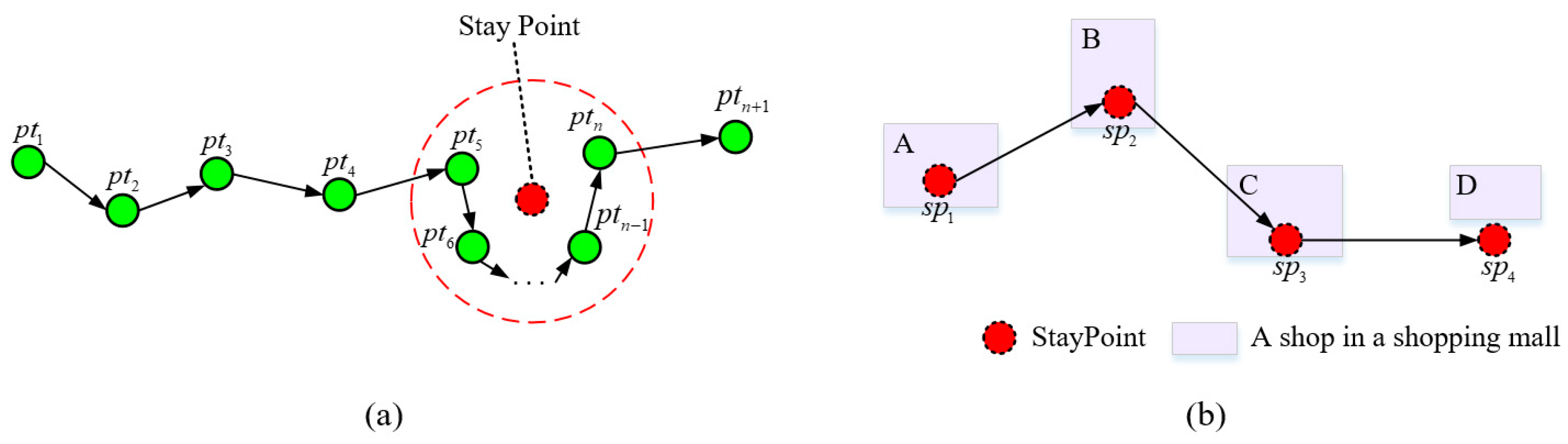
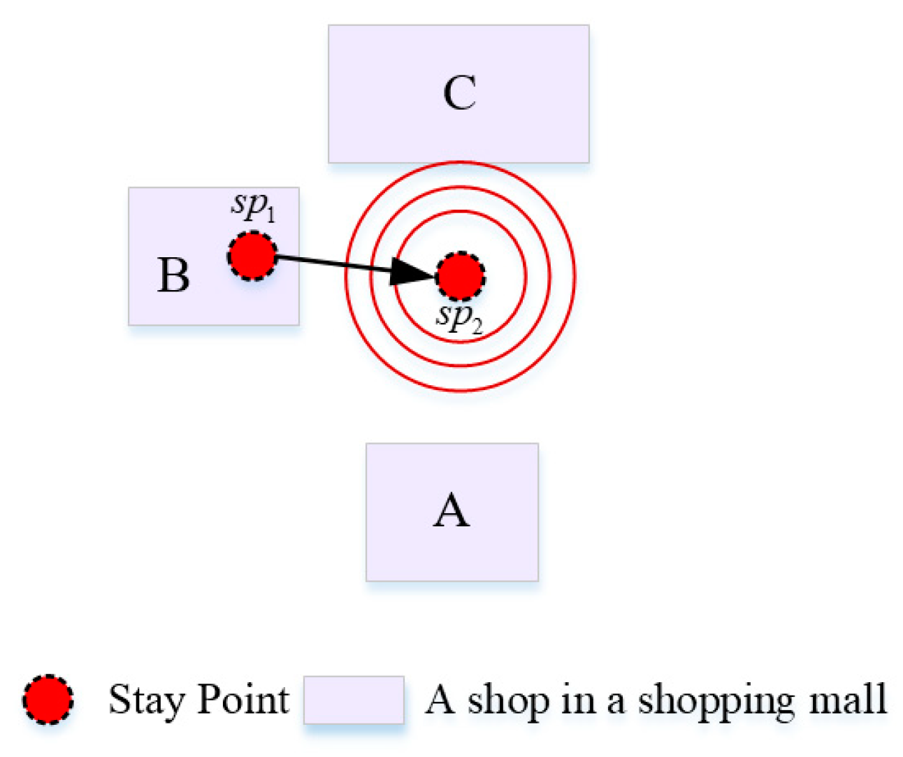
3.1.1. Stay Point Detection
| Algorithm 1. Indoor trajectory stay point detection algorithm. |
| Require: Individual trajectory: Radius: Time window: Neighborhood density threshold: Ensure: Individual stay point sequence: 1: function Indoor-STDBSCAN () 2: 3: for next unprocessed do 4: if then 5: continue 6: 7: if then 8: 9: 10: 11: for next do 12: 13: 14: if then 15: 16: 17: 18: for next do 19: 20: 21: 22: 23: return |
3.1.2. Location Sequence Conversion
3.2. Location Sequence Similarity Calculation Method
3.3. Indoor User Location Prediction Framework
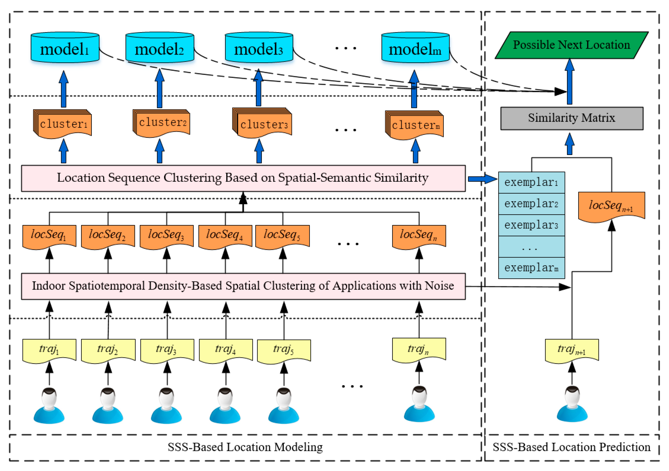
3.3.1. SSS-Based Location Modeling
| Algorithm 2. Training process of Indoor-WhereNext framework. |
| Require: Trajectories of All Users: Hyperparameters of Indoor-STDBSCAN: Weight coefficient: Ensure: Prediction models: Cluster centers: 1: for next do 2: 3: 4: 5: 6: 7: for do 8: 9: 10: return |
3.3.2. SSS-Based Location Prediction
| Algorithm 3. Prediction process of Indoor-WhereNext framework. |
| Require: New user trajectory: Hyperparameters of Indoor-STDBSCAN: Weight coefficient: α Prediction models: Cluster centers: Ensure: 1: 2: 3: 4: 5: 6: 7: return |
4. Experimental Results and Analysis
4.1. Data Preparation
4.1.1. Data Sources
4.1.2. Data Preprocessing
- (1)
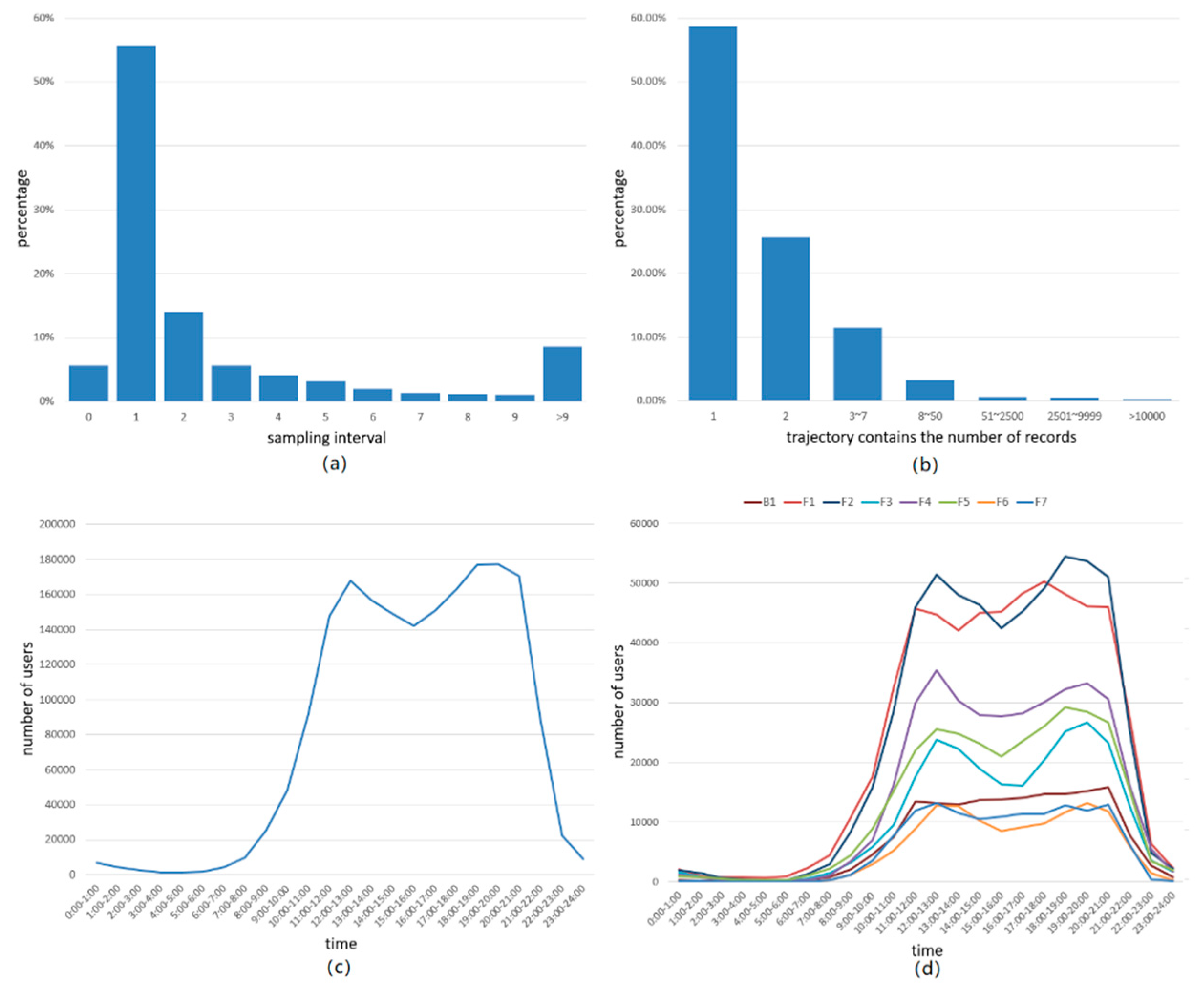
- The sampling interval for trajectory points was mostly concentrated between 1 and 5 s, accounting for approximately 82.5%, but there still were abnormal data with large sampling intervals and sampling intervals of 0 s. For example, trajectory points with sampling intervals of 0 s accounted for approximately 7.3%.
- (2)
- The number of trajectory points contained in a trajectory was between 1 and 7 in most sets, accounting for more than 97%. In other words, a large number of trajectories contained only a few trajectory points and could not be used to train the model. In our work, trajectories where the number of trajectory points was less than 50 were deleted.
- (3)
- The time span for trajectory points recorded in the shopping mall was 24 h—that is, there were records generated even during nonbusiness hours for the shopping mall, and the records generated in this process were invalid.
4.2. Evaluation Metrics
4.3. Variable Estimation
4.3.1. Calibrating the Parameters of Indoor-STDBSCAN
4.3.2. Calibrating the Weight Coefficient
4.4. Performance of Indoor-WhereNext
- (1)
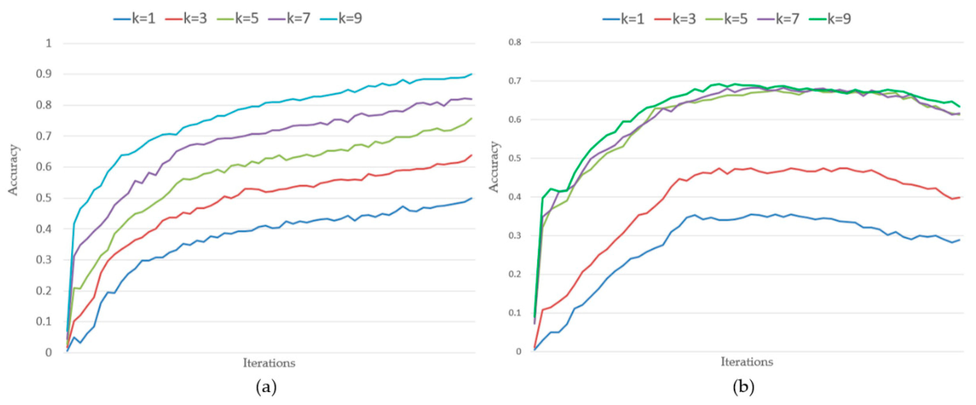
- For the training dataset, the prediction accuracy showed a continuous upward trend with the increase in the number of iterations.
- (2)
- For the test dataset, the prediction accuracy increased initially, then remained constant and finally decreased as the number of iterations increased. The framework tended to overfit as the number of iterations increased, improving the prediction accuracy of the model in the training dataset while worsening the prediction accuracy in the test dataset.
- (3)
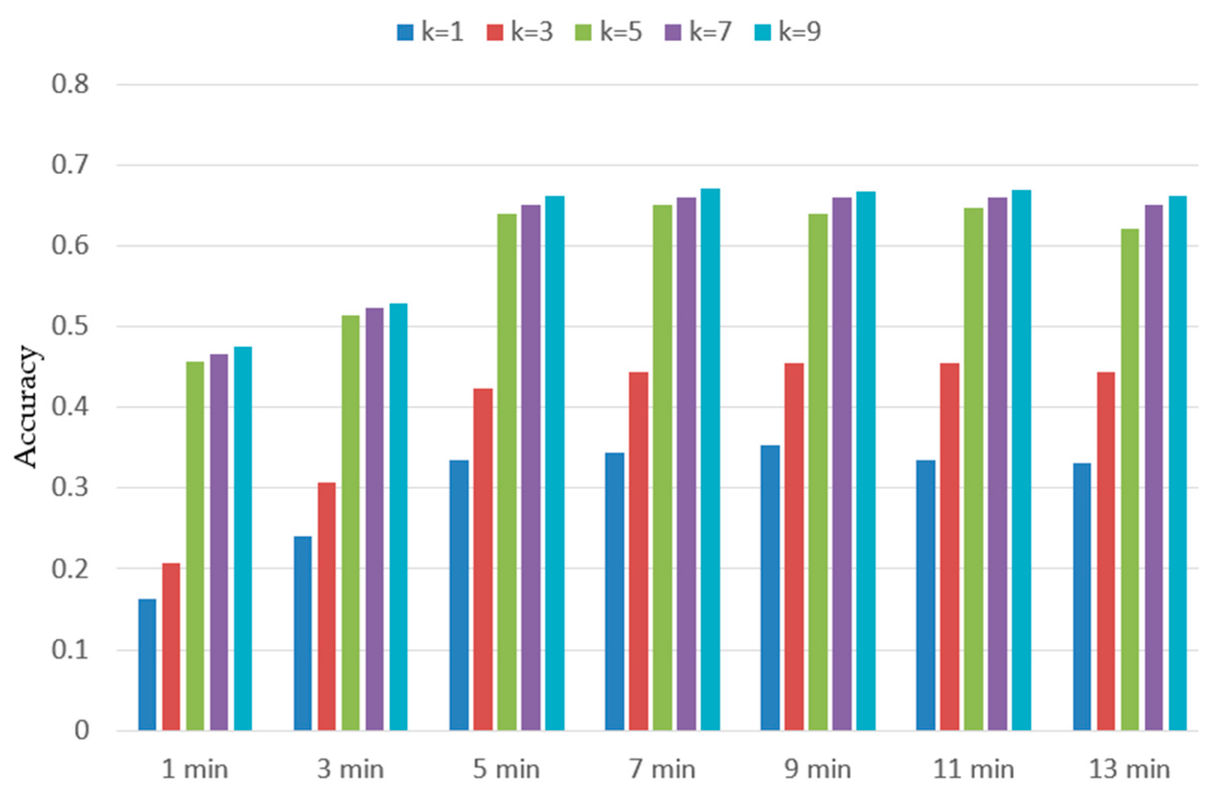
- Comparing on the test dataset, when , the prediction accuracy of the model was greatly improved; at , the prediction accuracy was 67.6%. Compared with and , the prediction accuracy increased by 32.5% and 22.1%, respectively. However, as continued to increase, the prediction accuracy of the model increased slowly. Compared with , and only increased by 0.9% and 1.5%, respectively, because the shop that the next user visits in the mall is often a collection of shops rather than a specific shop. In the predicted set of shops, the user destination has a certain randomness.
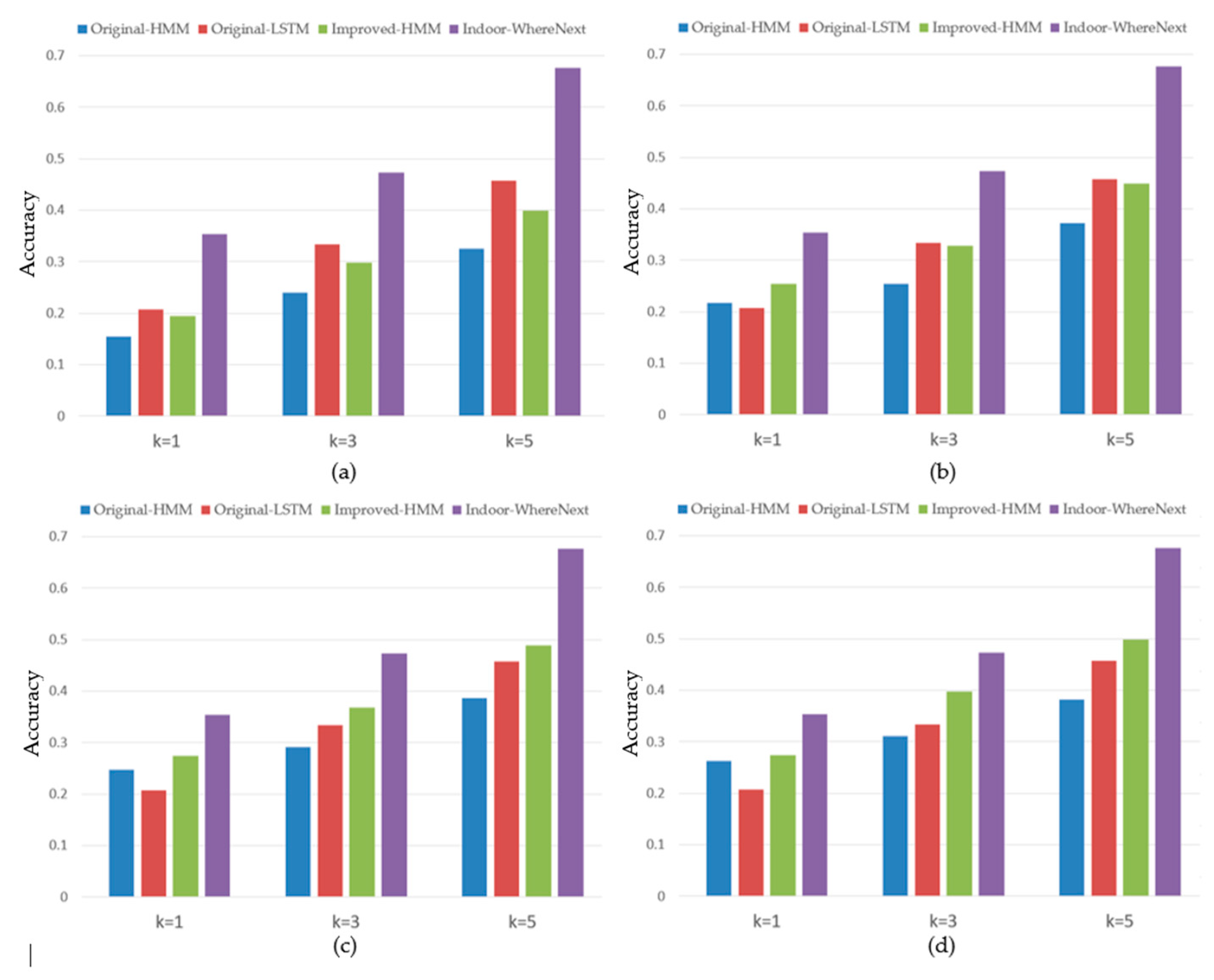
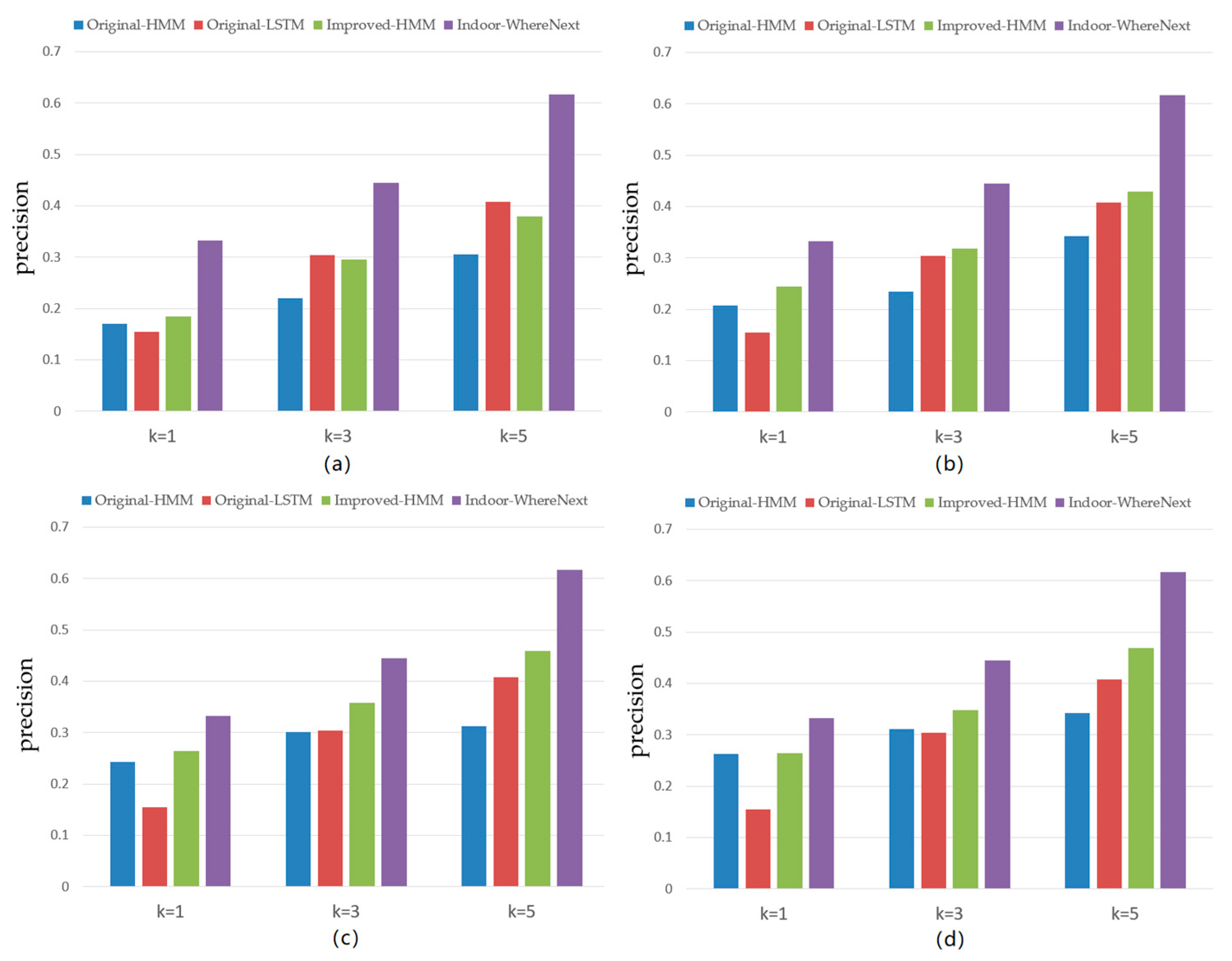
4.5. Comparison with Baselines
5. Conclusions and Future Work
Supplementary Materials
Supplementary File 1Author Contributions
Funding
Acknowledgments
Conflicts of Interest
References
- Wang, Y.-S.; Lin, S.-J.; Li, C.-R.; Tseng, T.; Li, H.-T.; Lee, J.-Y. Developing and validating a physical product e-tailing systems success model. Inf. Technol. Manag. 2018, 19, 245–257. [Google Scholar] [CrossRef]
- Hajli, N.; Featherman, M.S. Social commerce and new development in e-commerce technologies. Int. J. Inf. Manag. 2017, 37, 177–178. [Google Scholar] [CrossRef]
- Liu, Y.; Cheng, D.; Pei, T.; Shu, H.; Ge, X.; Ma, T.; Du, Y.; Ou, Y.; Wang, M.; Xu, L. Inferring gender and age of customers in shopping malls via indoor positioning data. Environ. Plan. Urban Anal. City Sci. 2019. [Google Scholar] [CrossRef]
- Zhang, H.; Wang, Z.; Chen, S.; Guo, C. Product recommendation in online social networking communities: An empirical study of antecedents and a mediator. Inf. Manag. 2018, 56. [Google Scholar] [CrossRef]
- Dixit, V.S.; Gupta, S.; Jain, P. A Propound Hybrid Approach for Personalized Online Product Recommendations. Appl. Artif. Intell. 2018, 32, 785–801. [Google Scholar] [CrossRef]
- Chan, N.N.; Gaaloul, W.; Tata, S. A recommender system based on historical usage data for web service discovery. Serv. Oriented Comput. Appl. 2012, 6, 51–63. [Google Scholar] [CrossRef]
- Tomazic, S.; Dovzan, D.; Škrjanc, I. Confidence-Interval-Fuzzy-Model-Based Indoor Localization. IEEE Trans. Ind. Electron. 2018, 66, 2015–2024. [Google Scholar] [CrossRef]
- Li, H.; Lu, H.; Shou, L.; Chen, G.; Chen, K. In Search of Indoor Dense Regions: An Approach Using Indoor Positioning Data. IEEE Trans. Knowl. Data Eng. 2018, 30, 1481–1495. [Google Scholar] [CrossRef]
- Guo, S.; Xiong, H.; Zheng, X.; Zhou, Y. Activity Recognition and Semantic Description for Indoor Mobile Localization. Sensors 2017, 17, 649. [Google Scholar] [CrossRef]
- Koehler, C.; Banovic, N.; Oakley, I.; Mankoff, J.; Dey, A.K. Indoor-ALPS:an adaptive indoor location prediction system. In Proceedings of the 2014 ACM International Joint Conference on Pervasive and Ubiquitous Computing, Seattle, WA, USA, 13–17 September 2014; ACM: New York, NY, USA, 2014; pp. 171–181. [Google Scholar] [CrossRef]
- Song, C.; Qu, Z.; Blumm, N.; Barabási, A.-L. Limits of Predictability in Human Mobility. Science 2010, 327, 1018–1021. [Google Scholar] [CrossRef]
- Lu, X.; Wetter, E.; Bharti, N.; Tatem, A.J.; Bengtsson, L. Approaching the Limit of Predictability in Human Mobility. Sci. Rep. 2013, 3, 2923. [Google Scholar] [CrossRef] [PubMed]
- Mingxiao, L.; Song, G.; Feng, L.; Hengcai, Z. Reconstruction of human movement trajectories from large-scale low-frequency mobile phone data. Comput. Environ. Urban Syst. 2019, 77, 101346. [Google Scholar] [CrossRef]
- Ye, M.; Yin, P.; Lee, W.-C. Location recommendation for location-based social networks. In Proceedings of the 18th SIGSPATIAL international conference on advances in geographic information systems, San Jose, CA, USA, 2–5 November 2010; ACM: New York, NY, USA, 2010; pp. 458–461. [Google Scholar] [CrossRef]
- Kuang, L.; Yu, L.; Huang, L.; Wang, Y.; Ma, P.; Li, C.; Zhu, Y. A Personalized QoS Prediction Approach for CPS Service Recommendation Based on Reputation and Location-Aware Collaborative Filtering. Sensors 2018, 18, 1556. [Google Scholar] [CrossRef] [PubMed]
- Bao, J.; Zheng, Y.; Mokbel, M.F. Location-based and preference-aware recommendation using sparse geo-social networking data. In GIS: Proceedings of the ACM International Symposium on Advances in Geographic Information Systems; ACM: New York, NY, USA, 2012; pp. 199–208. [Google Scholar] [CrossRef]
- Zhang, X.; Zhao, Z.; Zheng, Y.; Li, J. Prediction of Taxi Destinations Using a Novel Data Embedding Method and Ensemble Learning. IEEE Trans. Intell. Transp. Syst. 2019, 1–11. [Google Scholar] [CrossRef]
- Li, X.; Li, M.; Gong, Y.-J.; Zhang, X.-L.; Yin, J. T-DesP: Destination Prediction Based on Big Trajectory Data. IEEE Trans. Intell. Transp. Syst. 2016, 17, 2344–2354. [Google Scholar] [CrossRef]
- Bogomolov, A.; Lepri, B.; Staiano, J.; Oliver, N.; Pianesi, F.; Pentland, A. Once Upon a Crime: Towards Crime Prediction from Demographics and Mobile Data. In Proceedings of the 16th International Conference on Multimodal Interaction, Istanbul, Turkey, 12–16 November 2014; ACM: New York, NY, USA, 2014. [Google Scholar]
- Zhao, Z.; Koutsopoulos, H.N.; Zhao, J. Individual mobility prediction using transit smart card data. Transp. Res. Part Emerg. Technol. 2018, 89, 19–34. [Google Scholar] [CrossRef]
- Monreale, A.; Pinelli, F.; Trasarti, R.; Giannotti, F. WhereNext: A location predictor on trajectory pattern mining. In Proceedings of the Acm Sigkdd International Conference on Knowledge Discovery & Data Mining, Paris, France, 28 June–1 July 2009; ACM: New York, NY, USA, 2009; pp. 637–646. [Google Scholar] [CrossRef]
- Lee, S.; Lim, J.; Park, J.; Kim, K. Next Place Prediction Based on Spatiotemporal Pattern Mining of Mobile Device Logs. Sensors 2016, 16, 145. [Google Scholar] [CrossRef]
- Ying, J.C.; Lee, W.C.; Tseng, V.S. Mining Geographic-Temporal-Semantic Patterns in Trajectories for Location Prediction. ACM Trans. Intell. Syst. Technol. 2014, 5, 1–33. [Google Scholar] [CrossRef]
- Wu, R.; Luo, G.; Yang, Q.; Shao, J. Learning Individual Moving Preference and Social Interaction for Location Prediction. IEEE Access 2018, 6, 10675–10687. [Google Scholar] [CrossRef]
- Gambs, S.; Killijian, M.-O.; del Prado Cortez, M.N. Next Place Prediction using Mobility Markov Chains. In Proceedings of the 1st Workshop on Measurement, Privacy, and Mobility, MPM’12, Bern, Switzerland, 10 April 2012; ACM: New York, NY, USA, 2012. [Google Scholar] [CrossRef]
- Hawelka, B.; Sitko, I.; Kazakopoulos, P.; Beinat, E. Collective Prediction of Individual Mobility Traces for Users with Short Data History. PLoS ONE 2017, 12, e0170907. [Google Scholar] [CrossRef]
- Keles, T.I.; Ozer, M.; Toroslu, I.; Karagoz, P. Location prediction of mobile phone users using apriori-based sequence mining with multiple support. In Lecture Notes in Artificial Intelligence (Subseries of Lecture Notes in Computer Science); Springer: Berlin/Heidelberg, Germany, 2014; Volume 8983, pp. 179–193. [Google Scholar] [CrossRef]
- Morzy, M. Prediction of Moving Object Location Based on Frequent Trajectories; Springer: Berlin/Heidelberg, Germany, 2006; pp. 583–592. [Google Scholar] [CrossRef]
- Mathew, W.; Raposo, R.; Martins, B. Predicting future locations with hidden Markov models. In Proceedings of the UbiComp’12—2012 ACM Conference on Ubiquitous Computing, Pittsburgh, Pennsylvania, 5–8 September 2012; ACM: New York, NY, USA, 2012; pp. 911–918. [Google Scholar] [CrossRef]
- Qiang, L.; Shu, W.; Liang, W.; Tan, T. Predicting the next location: a recurrent model with spatial and temporal contexts. In Proceedings of the Thirtieth AAAI Conference on Artificial Intelligence, Phoenix, AZ, USA, 12–17 February 2016; AAAI Press: Palo Alto, CA, USA, 2016; pp. 194–200. [Google Scholar]
- Di, Y.; Chao, Z.; Huang, J.; Bi, J. SERM: A Recurrent Model for Next Location Prediction in Semantic Trajectories; ACM: New York, NY, USA, 2017; pp. 2411–2414. [Google Scholar] [CrossRef]
- Ye, Y.; Zheng, Y.; Chen, Y.; Feng, J.; Xie, X. Mining Individual Life Pattern Based on Location History. In Proceedings of the IEEE International Conference on Mobile Data Management, Taipei, Taiwan, 18–21 May 2009; pp. 1–10. [Google Scholar]
- Vu, L.; Do, Q.; Nahrstedt, K. Jyotish: Constructive approach for context predictions of people movement from joint Wifi/Bluetooth trace. Pervasive Mob. Comput. 2011, 7, 690–704. [Google Scholar] [CrossRef]
- Vu, L.; Nguyen, P.; Nahrstedt, K.; Richerzhagen, B. Characterizing and modeling people movement from mobile phone sensing traces. Pervasive Mob. Comput. 2015, 17, 220–235. [Google Scholar] [CrossRef]
- Do, T.M.T.; Dousse, O.; Miettinen, M.; Gatica-Perez, D. A Probabilistic Kernel Method for Human Mobility Prediction with Smartphones. Pervasive Mobile Comput. 2014, 20, 13–28. [Google Scholar] [CrossRef]
- Wu, F.; Fu, K.; Wang, Y.; Xiao, Z.; Fu, X. A Spatial-Temporal-Semantic Neural Network Algorithm for Location Prediction on Moving Objects. Algorithms 2017, 10, 37. [Google Scholar] [CrossRef]
- Zhou, Y.; Sun, H.; Huang, J.; Jia, X.; Zhao, Z. Efficient Destination Prediction Based on Route Choices with Transition Matrix Optimization. IEEE Trans. Knowl. Data Eng. 2018, 14. [Google Scholar] [CrossRef]
- Ang, B.-K.; Dahlmeier, D.; Lin, Z.; Huang, J.; Seeto, M.-L.; Shi, H. Indoor Next Location Prediction with Wi-Fi. In Proceedings of the Fourth International Conference on Digital Information Processing and Communications, Kuala Lumpur, Malaysia, 18–20 March 2014. [Google Scholar]
- Sepahkar, M.; Khayyambashi, M.R. A novel collaborative approach for location prediction in mobile networks. Wirel. Netw. 2018, 24, 283–294. [Google Scholar] [CrossRef]
- Zhang, D.; Zhang, D.; Xiong, H.; Yang, L.T.; Gauthier, V. NextCell: Predicting Location Using Social Interplay from Cell Phone Traces. IEEE Trans. Comput. 2015, 64, 452–463. [Google Scholar] [CrossRef]
- Wen, L.; Shi-Xiong, X.; Feng, L.; Lei, Z. Improving Location Prediction by Exploring Spatial-Temporal-Social Ties. Math. Probl. Eng. 2014, 2014, 1–7. [Google Scholar] [CrossRef]
- Li, J.; Brugere, I.; Ziebart, B.; Bergerwolf, T.; Crofoot, M.; Farine, D. Social Information Improves Location Prediction in the Wild. In Proceedings of the Workshops at the Twenty-Ninth AAAI Conference on Artificial Intelligence, Austin, TX, USA, 25–30 January 2015. [Google Scholar] [CrossRef]
- Spaccapietra, S.; Parent, C.; Damiani, M.L.; De Macedo, J.A.; Porto, F.; Vangenot, C. A conceptual view on trajectories. Data Knowl. Eng. 2008, 65, 126–146. [Google Scholar] [CrossRef]
- Ester, M.; Kriegel, H.P.; Sander, J.; Xu, X. A Density-Based Algorithm for Discovering Clusters in Large Spatial Databases with Noise. In Proceedings of the International Conference on Knowledge Discovery & Data Mining, Portland, OR, USA, 2–4 August 1996; Volume 96, pp. 226–231. [Google Scholar]
- Birant, D.; Kut, A. ST-DBSCAN: An algorithm for clustering spatial–temporal data. Data Knowl. Eng. 2007, 60, 208–221. [Google Scholar] [CrossRef]
- Iliopoulos, C.S.; Rahman, M.S. A New Efficient Algorithm for Computing the Longest Common Subsequence. Theory Comput. Syst. 2009, 45, 355–371. [Google Scholar] [CrossRef]
- Grover, A.; Leskovec, J. node2vec: Scalable Feature Learning for Networks. In Proceedings of the KDD: International Conference on Knowledge Discovery & Data Mining, San Francisco, CA, USA, 13–17 August 2016; pp. 855–864. [Google Scholar]
- Yuan, G.; Sun, P.; Zhao, J.; Li, D.; Wang, C. A review of moving object trajectory clustering algorithms. Artif. Intell. Rev. 2016, 47, 123–144. [Google Scholar] [CrossRef]
- Chen, L.; Özsu, M.T.; Oria, V. Robust and fast similarity search for moving object trajectories. In Proceedings of the 2005 ACM SIGMOD international conference, Baltimore, MD, USA, 14–16 June 2005; p. 491. [Google Scholar]
- Sankoff, B.D.; Kruskal, J.B. Time Warps, String Edits, and Macromolecules: The Theory and Practice of Sequence Comparison. Reading, MA: Addison-Wesley. J. Logic Comput. 1983, 11, 356. [Google Scholar]
- Frey, B.J.; Dueck, D. Clustering by Passing Messages Between Data Points. Science 2007, 315, 972–976. [Google Scholar] [CrossRef] [PubMed]
- Sepp, H.; Jürgen, S. Long Short-Term Memory. Neural Comput. 1997, 9, 1735–1780. [Google Scholar] [CrossRef]


| User ID | Date and Time | X (m) | Y (m) | Floor ID |
|---|---|---|---|---|
| 0000CE *** | 2017-12-31 10:46:45 | 130,219 *** | 43,904 *** | 1 |
| 0000CE *** | 2017-12-31 10:46:57 | 130,219 *** | 43,903 *** | 1 |
| 0000CE *** | 2017-12-31 10:47:05 | 130,219 *** | 43,904 *** | 1 |
| …… | …… | …… | …… | …… |
| 0000CE *** | 2017-12-31 19:20:33 | 130,219 *** | 43,904 *** | 4 |
| 0000CE *** | 2017-12-31 19:20:45 | 130,219 *** | 43,904 *** | 4 |
| Shop ID | Shape | Name | Floor ID |
|---|---|---|---|
| 1 | Polygon | *** | 2 |
| 2 | Polygon | *** | 2 |
| 3 | Polygon | *** | 6 |
| …… | …… | …… | …… |
| 488 | Polygon | *** | 4 |
| 489 | Polygon | *** | 3 |
© 2019 by the authors. Licensee MDPI, Basel, Switzerland. This article is an open access article distributed under the terms and conditions of the Creative Commons Attribution (CC BY) license (http://creativecommons.org/licenses/by/4.0/).
Share and Cite
Wang, P.; Wu, S.; Zhang, H.; Lu, F. Indoor Location Prediction Method for Shopping Malls Based on Location Sequence Similarity. ISPRS Int. J. Geo-Inf. 2019, 8, 517. https://doi.org/10.3390/ijgi8110517
Wang P, Wu S, Zhang H, Lu F. Indoor Location Prediction Method for Shopping Malls Based on Location Sequence Similarity. ISPRS International Journal of Geo-Information. 2019; 8(11):517. https://doi.org/10.3390/ijgi8110517
Chicago/Turabian StyleWang, Peixiao, Sheng Wu, Hengcai Zhang, and Feng Lu. 2019. "Indoor Location Prediction Method for Shopping Malls Based on Location Sequence Similarity" ISPRS International Journal of Geo-Information 8, no. 11: 517. https://doi.org/10.3390/ijgi8110517
APA StyleWang, P., Wu, S., Zhang, H., & Lu, F. (2019). Indoor Location Prediction Method for Shopping Malls Based on Location Sequence Similarity. ISPRS International Journal of Geo-Information, 8(11), 517. https://doi.org/10.3390/ijgi8110517