Article

An Intersection-First Approach for Road Network Generation from Crowd-Sourced Vehicle Trajectories

1
State Key Laboratory of LIESMARS, Wuhan University, 129 Luoyu Road, Wuhan 430079, China
2
Alibaba, Building No.9 Wangjing East Garden 4th Area, Chaoyang District, Beijing 100000, China
*
Author to whom correspondence should be addressed.
ISPRS Int. J. Geo-Inf. 2019, 8(11), 473; https://doi.org/10.3390/ijgi8110473
Submission received: 29 July 2019 / Revised: 7 October 2019 / Accepted: 21 October 2019 / Published: 24 October 2019

Abstract

:
Extracting highly detailed and accurate road network information from crowd-sourced vehicle trajectory data, which has the advantages of being low cost and able to update fast, is a hot topic. With the rapid development of wireless transmission technology, spatial positioning technology, and the improvement of software and hardware computing ability, more and more researchers are focusing on the analysis of Global Positioning System (GPS) trajectories and the extraction of road information. Road intersections are an important component of roads, as they play a significant role in navigation and urban planning. Even though there have been many studies on this subject, it remains challenging to determine road intersections, especially for crowd-sourced vehicle trajectory data with lower accuracy, lower sampling frequency, and uneven distribution. Therefore, we provided a new intersection-first approach for road network generation based on low-frequency taxi trajectories. Firstly, road intersections from vector space and raster space were extracted respectively via using different methods; then, we presented an integrated identification strategy to fuse the intersection extraction results from different schemes to overcome the sparseness of vehicle trajectory sampling and its uneven distribution; finally, we adjusted road information, repaired fractured segments, and extracted the single/double direction information and the turning relationships of the road network based on the intersection results, to guarantee precise geometry and correct topology for the road networks. Compared with other methods, this method shows better results, both in terms of their visual inspections and quantitative comparisons. This approach can solve the problems mentioned above and ensure the integrity and accuracy of road intersections and road networks. Therefore, the proposed method provides a promising solution for enriching and updating navigable road networks and can be applied in intelligent transportation systems.

1. Introduction

Digital road information is a pivotal part of basic geographic information and plays an important role in urban planning, intelligent transportation, and location services [1]. In the past, the collection of road information, mostly through traditional measurement methods, had a high cost of time and manpower. With the development of remote sensing technology, many scholars have proposed road extraction methods based on remote sensing images [2,3] and Light Detection and Ranging (LIDAR) point cloud data [4]. However, due to the mixture of multiple spatial information, road extraction is susceptible to interference. Additionally, the acquisition cost of remote sensing images and point cloud data is high and has a lag problem. Although it is possible to collect and edit data via a Mobile Mapping System, this method is also expensive, and road extraction information also often lags behind the latest changes in the actual road. With the development of the Internet and the popularity of GPS technology, the methods of geographic information acquisition have undergone tremendous changes. More and more locations can be reached via GPS or hand-held devices. Additionally, data are collected and uploaded by the public. These phenomena stimulate the generation of crowd-sourced trajectory data, which are acquired by soliciting contributions from a large group of volunteers. These data are different from those obtained by traditional measurement and remote sensing methods and have the advantages of being low cost, in real-time, and on a large scale, which is more suitable for the acquisition and rapid update of large-scale rural [5] and urban [6] road networks. At the same time, these data contain a large amount of driving record information, which makes a great contribution to the extraction of road-related geometry and attribute information, such as sidewalk networks [7], implicit entities [8], road boundary information [9], road slope and aspect information [10], and other road semantic information [11,12,13]. Therefore, the big real-time traffic data from crowd-sourced data not only make it a reality to extract a low-cost, fast-updating, highly detailed, and accurate road network, but can also mine a lot of road semantic information. This is a significant research field for road information extraction.
At present, existing studies dedicated to generating road maps from vehicle GPS traces are common and have made great progress. Previous work mainly focused on the extraction of the road skeletons, which can be divided into incremental methods [14,15,16], clustering methods [17,18,19], and raster methods [20,21]. Incremental methods combine routes one-by-one to form a graph [22], which starts from an empty road network, taking the first trajectory as the benchmark, and continuously adjusts and improves the initial road network by gradually inserting the trajectory. Clustering methods use some kind of clustering algorithm, such as K-means, to form a road network by considering the position or direction characteristics of the tracking points. Raster methods first rasterize the GPS track points to form a binary map and then use image-processing techniques to extract the road network.
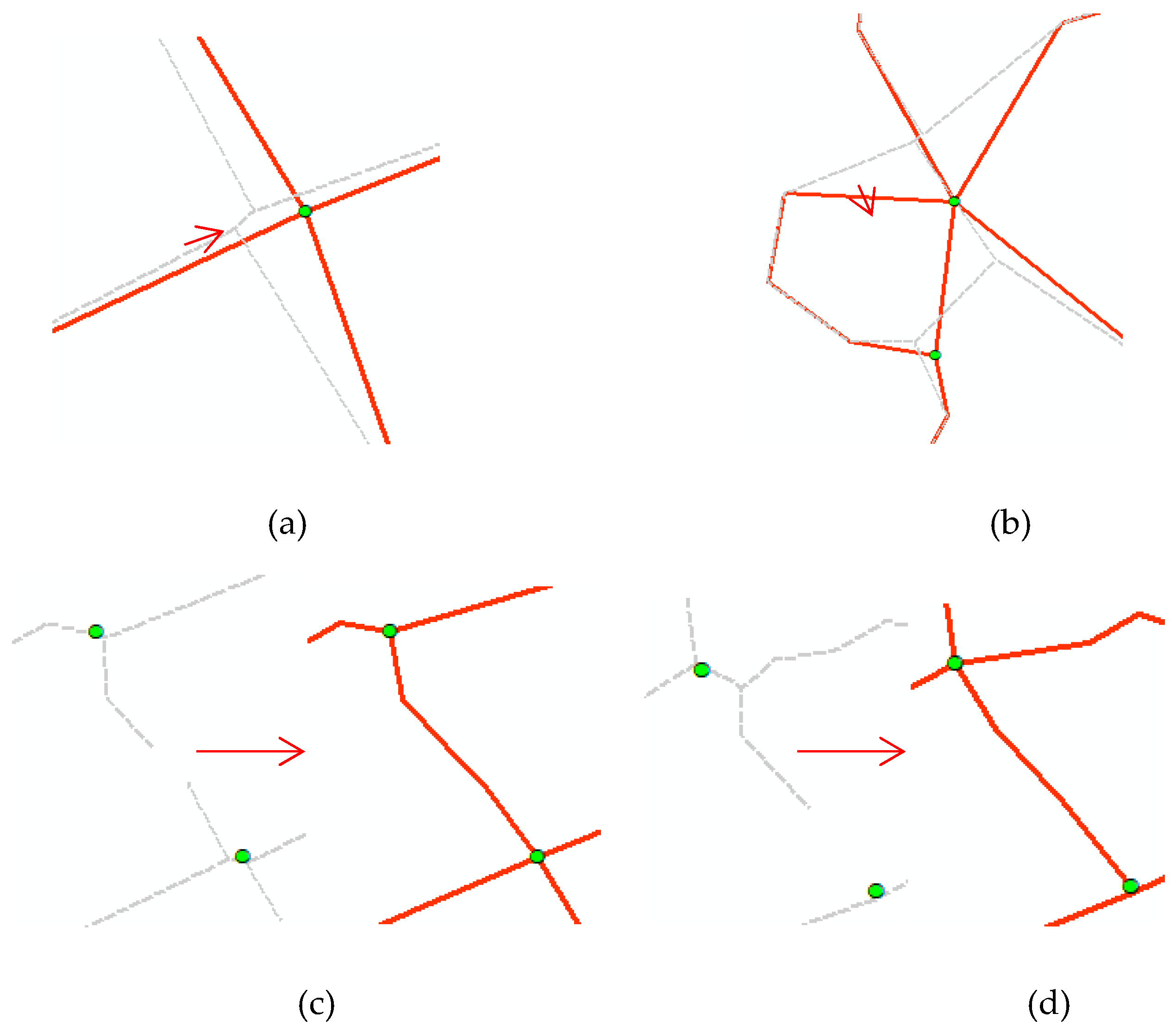
However, incremental methods are calculation-intensive and cannot determine the correct intersections. Clustering methods, on the other hand, have difficulty handling roads that are close in space. These two kinds of methods can only process high frequency, high precision, and high-density trajectories; they perform poorly for low frequency and high GPS error data. Even though the raster method can fit low-frequency trajectories, the precise geometry and correct topology of road networks cannot be guaranteed, and the morphology of a road is often distorted. As shown in Figure 1, the intersection position often deviates its right location and road segments around intersections with a few track points often distorted and broken.
To overcome the shortcomings of previous road data extraction methods based on the trajectory data, some studies argue that correct intersections can generate a high-quality road network, and some researchers have begun to do studies on the extraction of road intersections based on Longest Common Subsequence (LCSS) [23], heading direction changing [24,25,26,27], G index analysis [28,29], shape descriptors [30], etc. Additionally, some researchers [27,28,29] have attempted to extract turn rules based on clustering methods. However, the above road intersection extraction methods are either complex or inefficient [30], need to train a large number of data and build an empirical model to be viable, or are only applicable to high-frequency sampling data or high-density areas.
Therefore, there exist many challenges for road network extraction from crowd-sourced vehicle GPS trajectories, as follows:
First, high-frequency tracks are hard to obtain. Low-frequency tracks are more common, and most trajectory data are obtained by Commodity GPS devices in which the average sampling interval is more than 40 s, which means that the next points are often recorded after the vehicle passes one or more intersections. Thus, most methods mentioned above are inefficient for this kind of data.
Second, trajectory data are unevenly distributed, and road track points are intensive in traffic hub regions, while sparse in branch roads.
Third, the urban road network is extremely complex, as its intersections have multiple levels and types and may be too close to each other, meaning that the extraction of precise road segments around intersections cannot be guaranteed. Moreover, the morphology of a road is often distorted and broken for its low-frequency data properties.
In order to overcome the aforementioned challenges, a new intersection priority strategy to extract the road network using real-world vehicle GPS trajectory data was presented in this paper. We developed an integrated identification strategy focusing on the detection of road intersections and then constructed road improvement methods based on intersection results. The contributions of this paper are the following:
(1)
In grid space, we extracted the intersections by identifying the number of eight neighborhoods, per pixel, in the single-pixel “center-lines” and considered different resolutions, which can keep as many intersections as possible in our extraction method and also make the extraction results more accurate in the subsequent fusion processing.
(2)
In vector space, the clustering method to rapidly search for and find density peaks (CFDP) [31] was used to extract road intersections for the first time. Moreover, our method, which considers the distribution density of trajectory data and the traffic flow characteristic of roads, is available for both low-frequency and high-frequency trajectories, thereby solving the problem faced by other methods, such as heading and speed only being available for high-frequency trajectories.
(3)
An intersection fusion mechanism that integrates the advantages of cluster computing and image recognition was developed to overcome sampling sparseness and uneven distribution of the vehicle trajectory data. At the same time, this fusion mechanism can recognize true intersections and undetermined intersections, thereby guaranteeing the integrity of the extraction results and reducing the blindness of eliminating false intersections.
(4)
Making full use of the direct dependency between intersections and center-lines of the road can further adjust road information and repair fractured segments, thereby guaranteeing the precision of road segments around intersections. We also constructed an Intersection–Link model and used the road segment between intersections as the unit to identify single/double directional information and the turning relationships of the road network, to guarantee the precise geometry and correct topology of the road networks.
The remainder of this paper is organized as follows. 
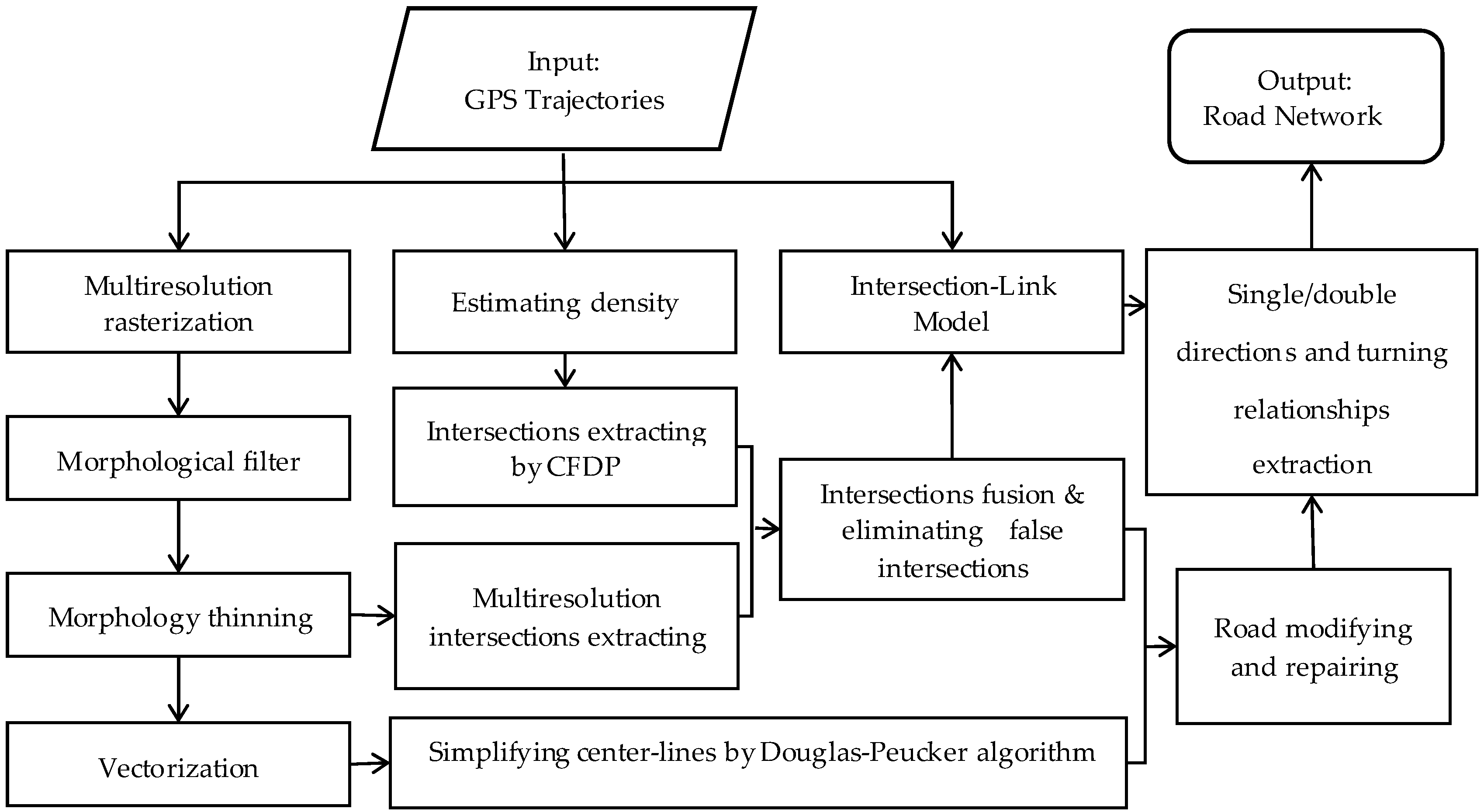
Section 2 describes the method’s flow and the strategy used to extract the intersections and build a road network. Section 3 outlines the procedure of our integrated intersection extraction method. Section 4 outlines the procedure of our method for building a road network. Section 5 presents a set of experimental analyses. Section 6 discusses the conclusions and suggestions for further work.

2. Road Network Generation Framework

On the one hand, intersections are key parts of a road network, as their effective identification is the basis of constructing a navigable road network. On the other hand, identifying road segments and turning relationships based on intersection extraction results is a divide-and-conquer method, which is helpful to reduce the difficulty of urban road network construction. However, the sampling frequency of crowd-sourced vehicle GPS trajectories is low, and its accuracy is not high. Furthermore, urban road networks are dense, and intersections are very close, so it is very challenging to construct urban road networks based on crowd-sourced vehicle GPS trajectories. This paper proposes an intersection-first approach for road network generation that uses low-frequency real-world vehicle GPS trajectories to correctly solve the above problems. According to our proposed road information extraction scheme, there are four key parts for obtaining road network information from GPS trajectories, as shown in Figure 2.
(1)
In the grid space, road intersections were extracted by identifying the number of pixels in each pixel’s eight neighborhoods from different resolution single-pixel “center-lines” to extract as many road intersections as possible. Before this, corresponding mathematical morphology processing, such as rasterization, open operation, close operation, filling holes, smoothing surfaces, and morphology thinning, needed to be done.
(2)
In the vector space, we considered the distribution density of the trajectory and extracted the road intersections via the clustering method of CFDP. In this critical part, in order to eliminate the trajectory points with large deviations caused by drift, Kernel Density Estimation (KDE) was first used to smooth the trajectory data.
(3)
In the aspect of integrated intersection extraction, a corresponding fusion mechanism was constructed. The true intersections and undetermined intersections were distinguished according to the fusion of the clustering results of the CFDP algorithm and the mathematical morphological extraction results from different resolution raster images. Finally, Principal Component Analysis (PCA) was used to analyze the undetermined intersections and detect the pseudo intersections so as to ensure the accuracy of eliminating the false intersections.
(4)
In terms of road network generation, a road improvement method was proposed to guarantee the precise geometry and correct topology of the road networks based on the above intersection extraction results. At the same time, we also designed the Intersection–Link model to identify the single/double direction information and turning relationships of the road network.

3. Integrated Intersection Extraction

Road intersections, which usually connect two or more road segments, are key parts of the road network. In this study, we extracted the road intersections first and then processed the road information. To ensure the accuracy and integrity of the result’s location, two methods were used to extract intersections. One method involves using mathematical morphology to calculate the trajectory raster images of different resolutions, and the other involves clustering the GPS trajectories to obtain the "road cluster point" via the clustering algorithm CFDP. The intersection results are obtained by fusing these two methods, so the intersection extraction is as complete as possible while the position maintains high accuracy.

3.1. Extracting Intersections under a Raster Space Using the Morphology Method

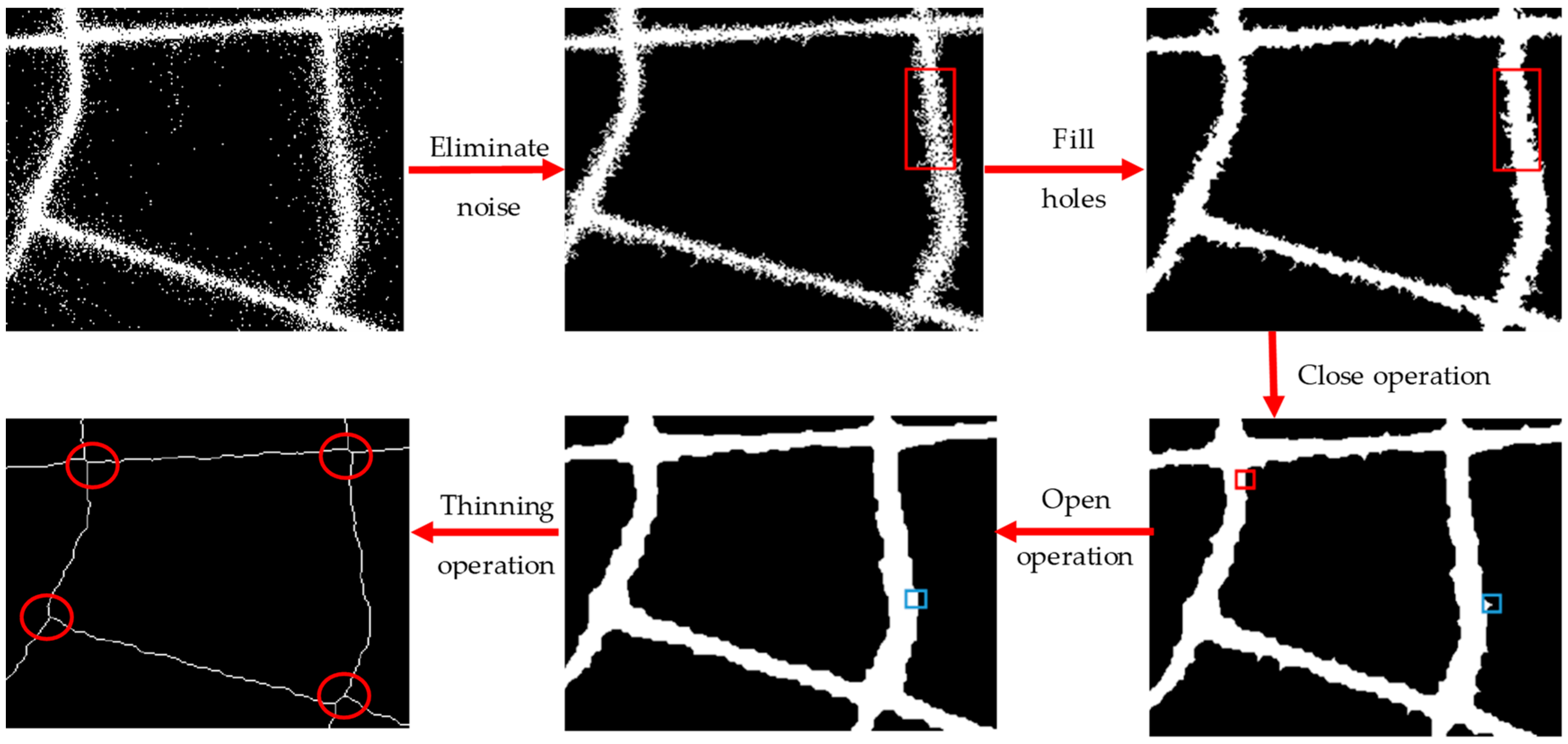
Mathematical morphology processing, which has been widely used in the road extraction of remote sensing images, is a computational method for grid space. Remote sensing images contain a variety of different spectral information, which have a great impact on road extraction, while images generated by rasterization based on taxi GPS trajectories are not interfered with by other ground information, thereby producing better results. In addition, using the mathematical morphology approach requires less time to process the trajectory data. Based on our observations, the cells in which the number of pixel points in eight neighborhoods is more than two in single-pixel “center-lines” have the greatest opportunity to be road intersections. As shown in Figure 3, cell a is an example of a road intersection, while cell b is an example of a non-intersection. In this study, we used the mathematical morphology method to obtain the single-pixel “center-lines” and extracted the intersections by identifying the number of pixels in each pixel’s eight neighborhoods.
The key steps for extracting road intersections via the morphological method are as follows:
Step 1: Rasterizing the GPS trajectories. In order to minimize the effects of noise, we set a statistical value c for each pixel based on the characteristics of a large number of track points, and specify that when a track point falls into a pixel of the raster image, the value of c for that pixel will be increased by 1. If the c value of a pixel is ultimately greater than or equal to the given threshold, the pixel value is set to 255; otherwise, the value is 0.
Step 2: Preprocessing the raster image. To accurately restore the shape of the original image, the etched image is used as the marker image and the original image as the mask image for the mathematical morphological reconstruction to eliminate outliers. At the same time, the reconstruction involves an iterative dilation process, which can ensure that holes are filled without changing the shape of the object. Operation preprocessing, such as open and close operations, can also be used to achieve image enhancement and smoothing, respectively.
Step 3: Extracting the single-pixel “center-lines” of the road by morphology thinning (shown in Figure 4).
Step 4: Calculating the number of pixels in each pixel’s eight neighborhoods in the thinning result. The pixels whose neighborhood numbers are more than two are considered as intersections.
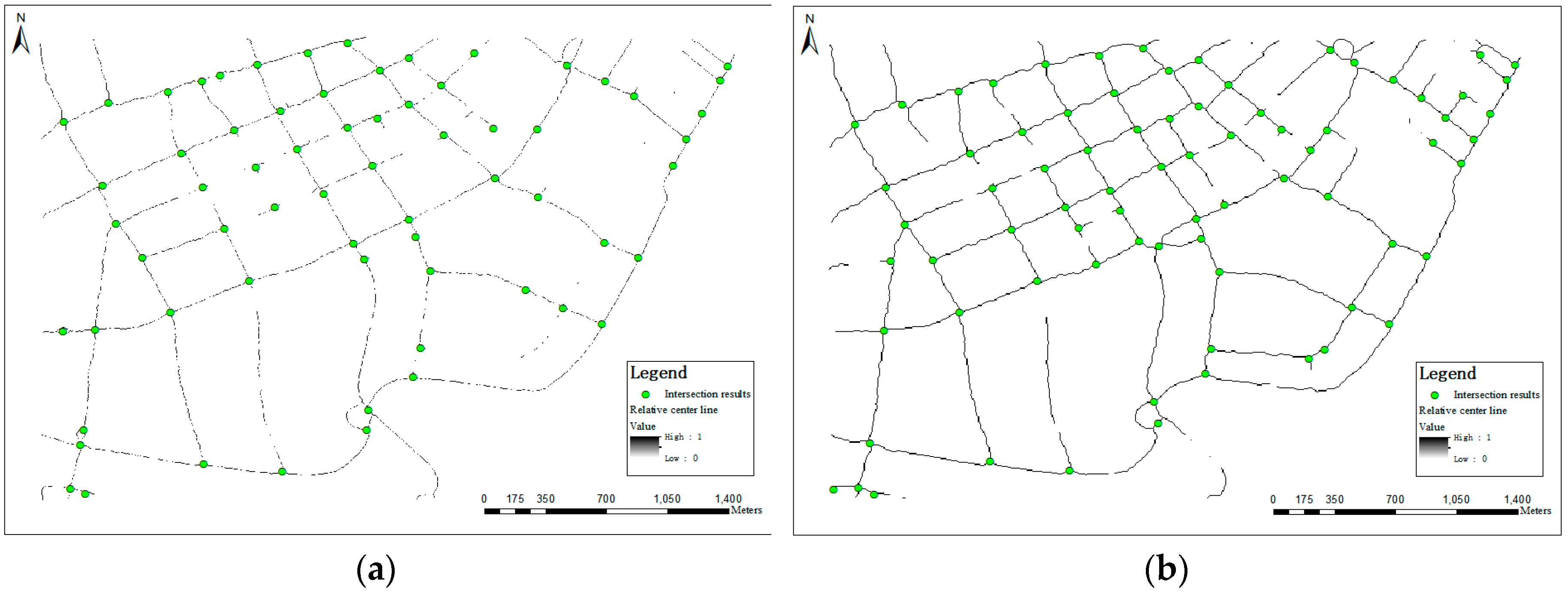
After preprocessing of mathematical morphology, the intersections can be obtained more accurately. However, when the trajectory points are rasterized, the resolution of the trajectory raster image will affect the final extraction result. Using a higher resolution, the location of the road can be reflected more accurately, as shown in Figure 5a. However, for areas where the track points are sparsely distributed, such processing may generate more outliers that will be treated as noise and eliminated. If using a lower resolution, as shown in Figure 5b, the proportion of trajectory pixels in the total number of pixels will increase, which facilitates the enhancement of sparse areas. Therefore, according to the strategy mentioned above, this paper uses high resolution and low resolution to extract road intersections, respectively, so our method can extract as many intersections as possible and also keep the extraction results more accurate in the subsequent fusion processing.
Urban road widths are diverse, ranging from 30 to 40 meters wide for main roads and 10 to 15 m wide for secondary roads. In order to accurately reflect the location of all roads and reduce the impact of noise, the raster resolution should not be too small. Therefore, two resolutions of 2.5 m and 5 m were selected for morphological processing. The intersection and center-line extraction results from different resolutions via rasterization using the Wuhan dataset are shown in Figure 6. The results show that the number of 2.5 m intersection extraction results is 66, the number of 5 m extraction results is 77, which is 11 more than the number of 2.5 m extraction results.
Even though the method considers sparse areas and sets different kinds of resolutions to extract intersections, it is still not suitable for less dense regions, as some center lines and intersections in sparse areas have still not been completely extracted. Therefore, it is necessary to combine the peak density clustering method and mathematical morphology method to extract the intersections to ensure the completeness of the results.

3.2. Extracting Intersections Under a Vector Space Based on CFDP

Due to the complexity of the intersections, a large number of GPS sampling points are gathered near the intersection so, although the GPS trajectories of some areas near intersections are sparse, the density clustering algorithm can be used to extract intersections. The CFDP clustering algorithm is used in this work because it captures the local maximum density positions of cells and is not easily disturbed by uneven track density distribution. Moreover, the CFDP algorithm has a few threshold settings. In contrast, DBSCAN merges proximal high-density cells into clusters; the mean shift algorithm is often affected by locally dense areas, and the results fluctuate greatly.
The GPS trajectory points in the study area range from thousands to millions, and the presence of discrete points (noise points) may result in the detection of false intersections. Since it is impossible to process the entire study area directly using the CFDP algorithm, KDE is used for data smoothing.

3.2.1. Estimating Density

KDE is used to calculate the density of the point elements, which represents the sum of the kernel functions that fall within the bump, as shown in Equation (1):
f ( x ) ^ = 3 m h 2 i = 1 m K ( 1 h ( x x i ) )
where m is the number of neighbor cells, xi is the center point of the ith cell, h is the bandwidth, and K(x) is the kernel function adopted in this work, as shown in Equation (2):
K ( x ) = { 3 π 1 ( 1 X T X ) 2 , X T X < 1 0 , o t h e r w i s e
In the density grid, large-value cells always exist within intersections, and small-value cells (also called noisy cells) usually exist at the margins of intersections or along roadways, as shown in Figure 7a. Based on the statistics of the density grid, we can acquire a statistical distribution map, as shown in Figure 7b. Setting the appropriate threshold K, we can extract the main road information, which consists of high-density cells for intersection detection.

3.2.2. Extracting Intersections

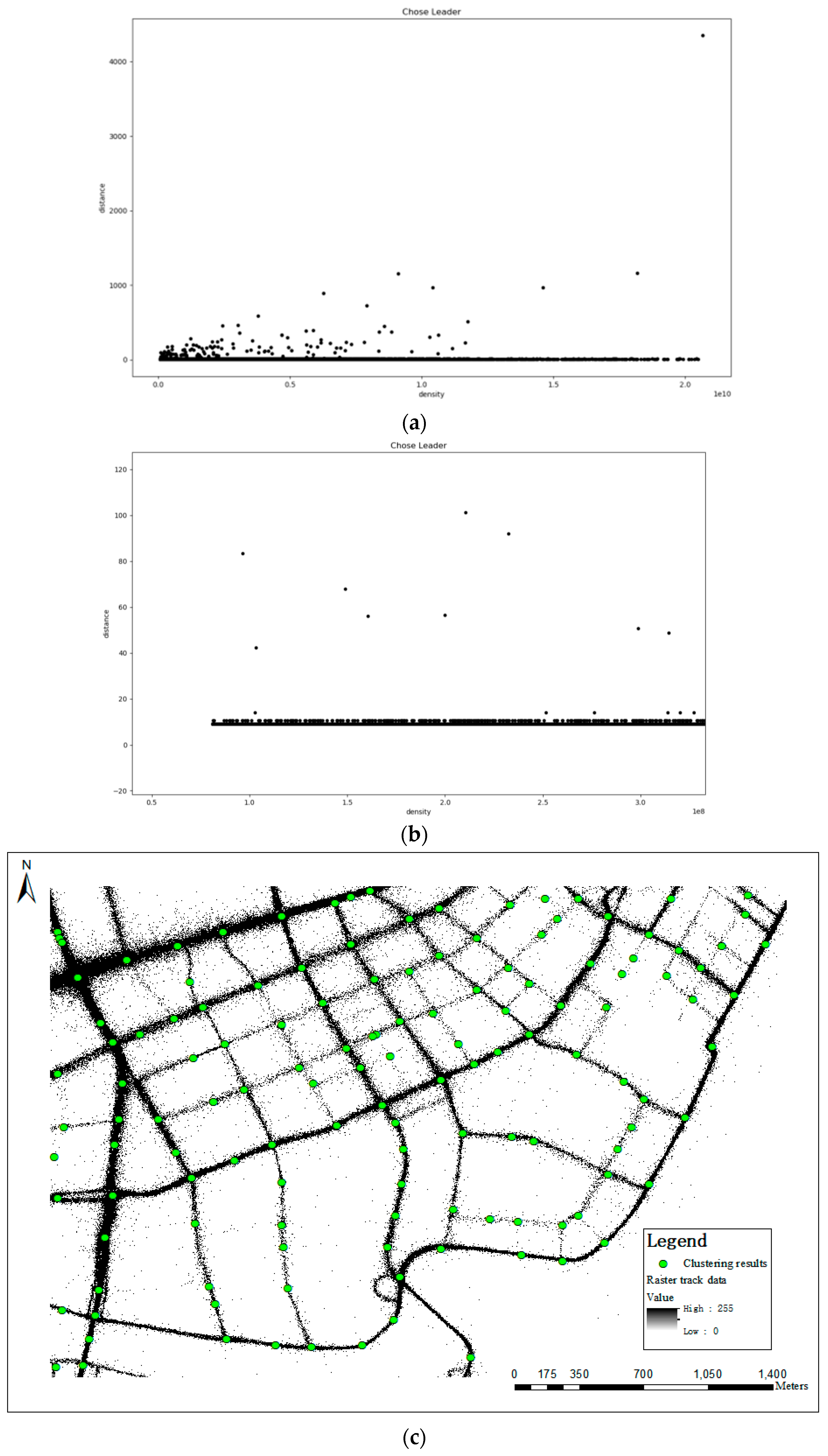
The CFDP algorithm is based on the assumption that the cluster center is surrounded by neighboring points with lower local densities and has a relatively large distance from any point with a higher density. Thus, for each point in the whole research region, two quantities are calculated: the local density of the point and the distance from the point to the point with a higher local density, both of which depend on the distance between the data points.
Based on estimating density processing, experimental data retains the main information about the intersection, and some noise points are removed while the number of data is reduced. Moreover, the extracted results have the density attribute { ρ i } i = 1 N . Then, let set { q i } i = 1 N denote a descending order of set { ρ i } i = 1 N . In other words, as ρ q 1 ρ q 2 ρ qN , then the point distance is defined as Equation (3):
δ q i = { m i n q j j < i { d q i q j } , i 2 m a x j 2 ( δ q j ) , i = 1
According to the decision diagram of the relationship between δ qi and ρ i , the cluster center, which is a candidate for intersection points, can be selected. Because the distribution of the GPS sampling points is inconsistent, if the distance and density threshold are considered at the same time, the sparse area extraction results will be affected, and the integrity of the extraction results will be reduced. Therefore, this paper takes into account the special qualities of intersections and only considers the distance threshold.
With the processing of the kernel density analysis, the data cluster is smoothed, and the distance within the cluster is suppressed. The larger the distance between the clusters, the more likely the intersection is. Amplifying the range of the red rectangular in the decision graph shown in Figure 8b, we can see that the distance of many points clusters under 20 meters. Thus, setting the distance threshold D as 20 meters, the extraction results using the Wuhan dataset via the CFDP algorithm are shown in Figure 8c. The extraction of the intersection is only related to distance, which solves the difficult parameter adjustment problems.

3.3. Fusion and Eliminating Pseudo Intersections

In order to reduce the blindness of eliminating pseudo intersections and ensure the integrity and accuracy of the extracted intersections, this paper establishes a corresponding fusion mechanism based on the extraction results of different methods to distinguish between true intersections, pseudo intersections, and undetermined intersections. This study also uses PCA to eliminate pseudo intersections. The road intersections fusion frame is shown in Figure 9.

3.3.1. Fusion of the Intersection Extraction Results

Considering the density characteristics of the road intersections compensates for the morphology extraction results, but also results in some pseudo intersections. Consequently, we proposed a variety of fusion rules (listed in Table 1) based on our extraction results, including high-resolution results, low-resolution results, and CFDP clustering results, to help recognize the undetermined results and reduce the error rate of eliminating pseudo intersections. If only high-resolution results or low-resolution results are present within the distance of a given fusion threshold R1, then the intersections are false. If only the CFDP clustering results are present, then the intersections are undetermined. In other situations, the fusion results are based on the high-resolution results (if they exist). Otherwise, the fusion results are based on the low-resolution results.
Based on the above rules, we set 80 meters as the fusion threshold value. The fusion results distinguish 79 true intersections, 4 false intersections, and 57 undetermined intersections, which are shown in Figure 10.
Undetermined results all come from clustering results that greatly supplement the raster extraction results, especially the intersections of the residential streets, living streets, and pedestrian streets that have no (or few) taxi tracks. However, the congestion in some sections of the road and long taxi stays result in a large number of loci, and some pseudo intersections have also been extracted. We also extracted a method to eliminate the pseudo intersections, focusing on the undetermined results.

3.3.2. Elimination of False Intersections from Undetermined Results

Pseudo intersections (that is, non-real intersections) that are identified as intersections may be caused by taxis stopping, cars turning at gas stations, viaducts, or other special road landmarks. For this reason, we use the PCA method to analyze the linear significance of spatial distribution near undetermined intersections, which are extracted based on the above fusion rules to further distinguish pseudo-intersections from undetermined intersections. First, we created a circular buffer with radius R2 at the undetermined intersection to collect the track points falling into the circular buffer. Then, we construct a covariance matrix by taking x and y coordinates from the set of track points as variables and calculate the eigenvalues λ1 and λ2 of the matrix. Finally, we use Equation (4) to judge the main direction of traffic flow at the undetermined intersections and the intensity in each direction. It is obvious that the larger the Δ, the stronger the linear feature, which means the less likely it is to become a true intersection, as shown in Figure 11. In order to retain more true intersections, we can choose the larger Δ value as the threshold value to filter the intersection points. Δ is calculated based on the following formula:
Δ = max ( λ 1 , λ 2 ) min ( λ 1 , λ 2 ) max ( λ 1 , λ 2 )

4. Road Network Generation

According to the above work, we extracted the single-pixel “center-lines” of the road by morphology thinning. Our goal was to produce an initial road map consisting of nodes and edges. Thus, we first vectorized the skeleton image and used the Douglas–Peucker algorithm [32] to produce the edges that make up the shape of each road segment. Secondly, in order to determine the road integrity and topological consistency, we used the extracted intersections to adjust the distorted road segments around the intersection and connected the fracture segments to guarantee the road network’s accuracy. Finally, we designed the Intersection–Link model and took the road segments between the intersections as the units to identify the single/double directions and turning relationships of the road network.

4.1. The Road Improvement

The road segments around the intersections are distorted and broken. In this section, we build buffers for intersections. We set 80 m (the same as the fusing threshold R1) as the buffer radius and designed the specific algorithm to adjust the roads’ endpoints falling into the buffer of the relative intersections to correct the position and shape of the road segments around the intersections, as shown in Figure 12a,b. At the same time, we also connected the fractured segments according to the broken segment’s distance and direction deviation, or the distance and direction deviation between the broken segment and the relative intersection, by using extracted intersection results, as shown in Figure 12c,d.
Except for the intersection extraction results of set I in this stage, this connecting strategy requires to detect the suspension points set S and the suspension lines set L and to calculate the following two parameters: dis(pm,pn) < 500 m or dis(pm,Pi) < 500 m and dir(lm, (pn-pm)) < 30o or dir(lm, (Pi-pm)) <30o, where p m , p n S , m , n = 0 , 1 , 2 , , m n , P i I , i = 0 , 1 , 2 , , l m . The point that satisfies the above conditions and has the minimum distance will be selected to connect the suspension point. These parameters were determined based on the distance and direction between fractured segments as well as after much experimental exploration to yield the best results.

4.2. Identifying Single/Double Directions and Turning Relationships

A road intersection is an intersection of two or more roads that divide the urban road network into sections of moderate length without overlapping. Therefore, we designed the Intersection–Link model and used the road segment between intersections as the unit to identify the single/double directions and turning relationships of the road network.

4.2.1. Intersection–Link Model Construction

Building the Intersection–Link model is a process of track segmentation. A track is divided into several sections according to the road intersections, and each pair of adjacent road intersections corresponds to multiple track segments. Denoting any two adjacent road intersections in the node set as Ik and Ij, traversing the original track data, and calculating all n track segments between them, the Intersection–Link model can be obtained:
(Ik , Ij) ~ {t1,t2,t3,…,tn}.
Here, tk(0<k≤n) represents the information of a track segment between Ik and Ij, which are two adjacent road intersections, including track ID and the track point coordinate information.
The Intersection-Link model’s construction is used to assign the original track points to an adjacent road intersection. For any track, it is necessary to determine which point passes through a road intersection. If two points in the track pass through two road intersections successively, then the point between them belongs to the section between these two intersections.

4.2.2. Removing the Pseudo-Intersection–Link Relationship

Due to the low sampling frequency of the track data, some tracks may cross several sections before passing through a road Intersection, thereby forming a pseudo-Intersection–Link relationship. Then, we adopted the following strategies to eliminate the pseudo-Intersection–Link relationship:
  • We use the straight line connecting the two road intersections as the diameter to establish the circular buffer zone. If there are too many other intersections in the buffer, the two intersections are too far apart. If so, delete the Intersection–Link relationship of the two intersections.
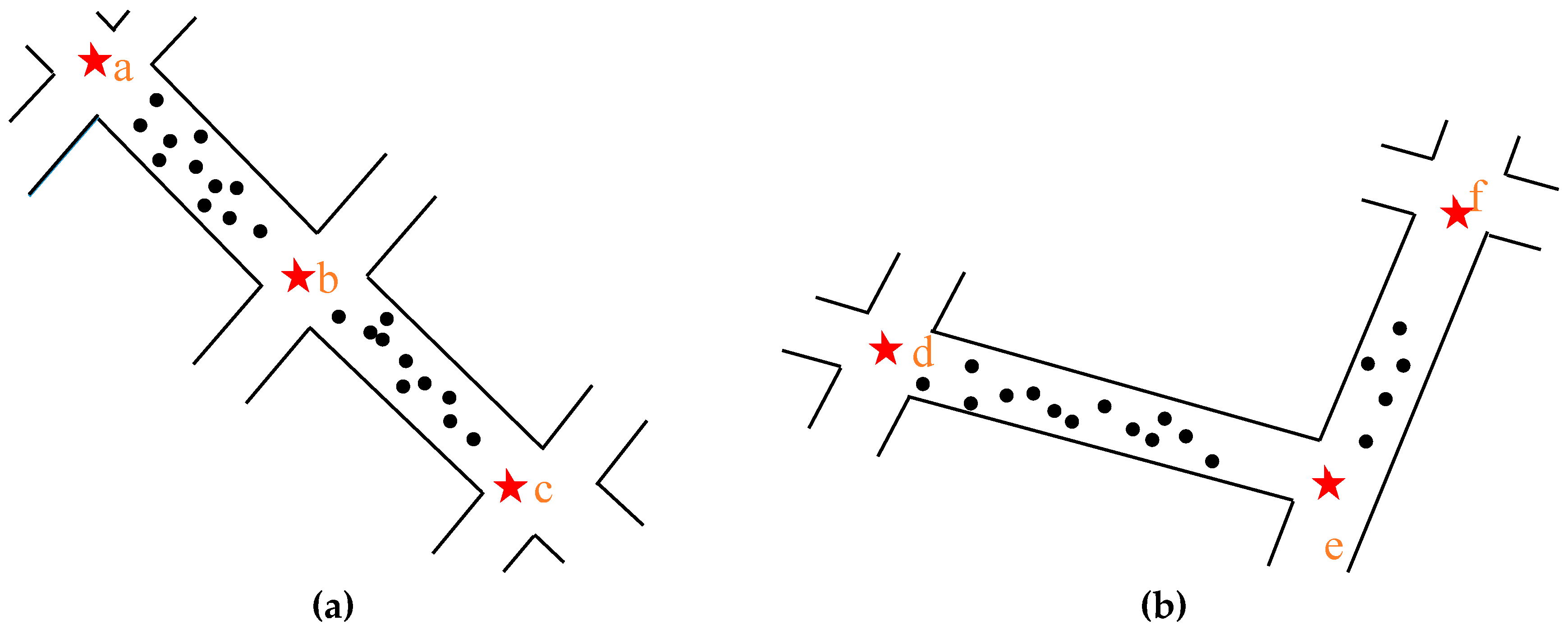
  • The Intersection–Link relationships are formed between two of the three road intersections (such as a, b, and c), which are located in the same straight line. The lengths of ab, ac, and bc were calculated accordingly to eliminate the Intersection–Link relationship of the longest pair of intersections, as shown in Figure 13a.
  • Most sections of urban roads are straight lines, while some sections have small radians. Based on this observation, the maximum distance d from the intersection line (let the length be L) in the normal track points is calculated. If d/L is greater than the threshold, then delete the Intersection–Link relationship. This strategy can eliminate the situation seen in Figure 13b.

4.2.3. Determining the Characteristics of a Road Network

The Intersection–Link model shows the relationship between road segments and track segments, which can be used to identify the single/double directions and turning relationships of the road network. Suppose the start-and-end intersections of a road section are a and b, respectively. The Intersection–Link relationship only exists between a to b or b to a, indicating that this road section is a single-lane road section. The Intersection–Link relationship exists between a to b and b to a, indicating that the road section is a two-way road section. Take road intersection 3 in Figure 14 as an example. Intersections 2 and 3 have an Intersection–Link relationship. Intersections 3 and 4 have an Intersection–Link relationship at the same time, which is insufficient to indicate that there is a turning relationship between the two sections. Thus, the track segment in two Intersection–Link relationships needs to be checked. If the track segment between intersections 2 and 3 belongs to the same track as the track segment between intersections 3 and 4, and the vehicle’s time from intersection 2 to 4 does not exceed a certain threshold, then it can be determined that there is a turning relationship between section A and section D at intersection 3. It is worth mentioning that the number of intersections that can be used for turning at road intersections is often more than those that cannot be used for turning, so the selection of storage turning restriction relationships can effectively improve the storage efficiency.

5. Experiments and Analysis

5.1. Study Area and Data Sets

Real-world vehicle trajectory data for seven days from May to June 2014 in the Wuhan city and Chicago Campus Bus Datasets were used to test the feasibility and effectiveness of the proposed intersection extraction method and road construction method. Both of them include the following main fields: vehicle ID; time; longitude; latitude; speed (m/s); and heading (degree), which is relative to north.
Wuhan dataset covers a region of 4.2 km × 2.8 km, containing about 2000 taxi trajectories and nearly 800,000 trajectory points. The average sampling interval of the dataset is more than 40 seconds. The experimental area is an old central urban area near Hankou in Wuhan city, and the track points are unevenly distributed on different volume roads with significant noise, as shown in Figure 15a. Part of the dataset can be shown in Figure 15c. The Chicago dataset, which has been widely used in related work [33] and is available on the website [34], is relatively clean and contains 118,364 GPS points and 889 trajectories within a region of 3.88 km × 2.4 km at the University of Illinois in Chicago, as shown in Figure 15b.

5.2. Experimental Results of the Proposed Method

Based on the approach described above, we developed a set of programs to generate intersections and road networks from vehicle GPS trajectories using Python and C# via the ArcEngine platform.
The experimental parameters involved in this experiment include the size of the structural elements S during morphological operations, kernel density threshold K, clustering distance threshold D, fusing threshold R1, circular buffer radius R2, and the threshold Δ of eliminating false intersection points. In order to extract more intersection points, the close operation uses larger structural elements, the open operation uses smaller structural elements, and Δ needs to be set to the larger value. The kernel density threshold can be set according to the quantile classification method. For the Wuhan dataset, K was set to 25% of the maximum kernel density. For the Chicago dataset, K was set to 100% of the maximum kernel density. Since the distribution of the Chicago dataset is relatively even and the dataset has few noises, the threshold of K is reasonable for the Chicago dataset, which also indicates the feasibility of the quantile classification method. Clustering distance threshold D and fusing threshold R1 are related to the spacing of road intersections at all levels, so they can be set according to the minimum spacing planning for road intersections in relative research areas. However, in a situation in which the distance δ qi of many points clusters under a certain distance, as shown in Figure 8, the clustering distance threshold needs to be set as the corresponding distance for more extraction results. The circular buffer radius R2 was empirically set to 100. The parameter settings for the experiment are shown in Table 2.

5.2.1. Intersection Detecting Results

The extraction results of the road intersections in Chicago and Wuhan are presented in Figure 16a,b. After PCA analysis and the elimination of false intersections from the undetermined results, a total of 117 and 51 intersections were detected from the Wuhan dataset and Chicago dataset, respectively. Overlaying the final extraction intersections, the remote sensing image and 2.5 m raster track data revealed a good fit with the map, as shown in Figure 16. Compared with the morphology method alone, the fusion method not only ensures the integrity of the results but also confirms the correction of the extraction results. Greater than 90% of the detected results are true intersection points, indicating that our methods can correctly distinguish a variety of road intersections from other roadways.
However, there are also some road intersections not being detected due to having insufficient GPS data. As shown in Figure 16, there are non-existent, or few taxi tracks passing residential streets, living streets, and pedestrian streets, so some of these types of road intersections cannot be extracted. Though our method complements some kind of these intersections, it’s still a challenging task to recognize all intersections only using taxi tracks. This issue could be solved by considering walking trajectory data.
Finally, due to the uneven distribution of primary and secondary roads in some areas, a few false intersections could not be removed by the PCA method. Meanwhile, the PCA method, which is used to determine false intersection points according to their linear characteristics, can not apply to the turning area.

5.2.2. Road Network Detection Results

Due to the serious absence of the road information for 2.5 m resolution thinning images, we vectorize and simplify the 5 m resolution thinning image to get the vector road center-lines by using the Douglas–Peucker algorithm. The results, according to road reprocessing, are shown in Figure 17. Almost all the roads that taxi tracks pass through can be extracted. The roads that are residential streets, living streets, and pedestrian streets with no taxi tracks also could be extracted by fusing the walking trajectory data. We must mention that some extracted road segments are seriously distorted simply because the road segments are too close to each other or do not have enough trajectory points to form the correct road shape. These are all difficult problems for current research.

5.2.3. Single/Double Direction Information and Turning Relationship Detection Results

The Intersection–Link relationship can be used to extract the single/double direction information and turning relationship of the road network. Taking intersection 69, extracted from the Wuhan dataset, as an example (shown in Figure 18), the result of this relationship is shown in Table 3 and Table 4.
According to the Intersection–Link model, we can determine which road sections and road intersections the track passed and then extract the single/double direction information, as well as the turning relationship, of the road. Where the viaduct passes, it may form an area with a pseudo-intersection, which can also be recognized by the Intersection–Link model.

5.3. Results Evaluation and Analysis

In this section, we compare our proposed method with the aforementioned method proposed by Ahmed [15] and Davies [20]. For Ahmed, the values of ε to the cluster sub trajectories are 140 and 80 m for Wuhan and Chicago, respectively. The parameter of the proximity for Davies’ algorithms is 17 m. Directly using the Wuhan dataset to extract the road network via the methods of Ahmed and Davies cannot achieve appropriate results for low-frequency data. Therefore, in this experiment, the Delaunay triangulation method [35] was used for the Wuhan dataset preprocessing, and then we extracted the trajectory points within 60 s and deleted the trajectory whose number of track points fewer than two.

5.3.1. Visual Inspection

Figure 19 shows the detection results from Ahmed’s method and Davies’ method. Compared with the extraction results from the proposed method shown in Figure 16 and Figure 17, these two methods did not extract more road intersections and skeleton information, and a lot of results deviated from their correct positions. For the Chicago dataset, although Ahmed’s method extracted more skeleton information, it produced a large number of offset and messy outputs. The visualization clearly shows that the proposed method is better than the other two methods.

5.3.2. Quantitative Comparisons

We also use precision, recall, and the F-value to evaluate our method. Accuracy comparison for detecting road intersections can be shown in Table 5. The proposed method achieved a significantly higher precision value and F-value than the method of Ahmed and Davies, which demonstrates superior performance for detecting road intersections. Three indicators were computed utilizing Equation (5):
Precision = c o r r e c t l y   d e t e c t e d c o r r e c t l y   d e t e c t e d + i n c o r r e c t l y   d e t e c t e d
Recall = c o r r e c t l y   d e t e c t e d c o r r e c t l y   d e t e c t e d + n o t   d e t e c t e d
F value = 2 * p r e c i s i o n * r e c a l l p r e c i s i o n + r e c a l l
According to the visual inspections and quantitative comparisons, we can see that the proposed method extracted more intersections and has considerable consistency with the remote sensing image. At the same time, the road extraction results also show more accurate and richer information, especially for the Wuhan dataset, which contains low-frequency data. However, based on the results in Table 4, there was also about a 2% and 7% chance of incorrectly identifying road intersections, and about 30% and 20% of the road intersections were not identified for the Chicago dataset and the Wuhan dataset, respectively.
For further observation of the extraction results, we overlay the final extraction results, Open-street Map (the blue line is the urban traffic roads, the yellow line is the urban living streets), 2.5 m raster track data and remote sensing image, as shown in Figure 20. The incorrectly identified intersections are mainly concentrated on elevated road entrances and exits, sharply curved points, points close to living streets, and points of interest where cars are parked for a long period. We can consider random forest and other technologies to further improve the accuracy of eliminating pseudo intersections. In fact, these special false intersections are also important for navigation. We can consider distinguishing these points in future work and provide a reminder service for the navigation user. Thus, further analyses and improvements are still needed.
Based on the results shown in Figure 16, the road intersections, which were not identified, are mainly the intersections of the residential streets, living streets, and pedestrian streets that have no (or few) taxi tracks. Although our method complements some of these intersections, it is still a challenging task to recognize them all only using taxi tracks. This issue can be solved by considering walking trajectory data.
There also remains a small amount of road skeleton information that was not extracted for the Chicago dataset and Wuhan dataset, which can be fitted via Multivariate Adaptive Regression Splines (MARS) according to the intersection results and the Intersection–Link model, as shown in Figure 21.
In addition, time-cost is an important factor to be considered in algorithm application. Since the overhead of the CFDP algorithm is O(n3), our method has a larger time cost compared with the methods of Ahmed and Davies. It took about five and seven hours longer than them to extract road information based on the Wuhan and Chicago datasets, respectively, even though we had considered the kernel density estimation to smooth the data and reduce the amount of data calculation. Despite this, compared with some incremental methods (such as Cao’s method [14]) and neural network methods (such as Fathi’s method [30]), the overhead of our method is not so bad, because these methods may take dozens of days. Parallel computing will be considered to solve this problem in the future.

6. Conclusions

Crowd-sourced Vehicle Trajectories have the disadvantage of lower accuracy, lower sampling frequency, more noise, and uneven distribution, which makes it more difficult to determine a road network than in most existing approaches that use high precision and high-frequency GPS trajectories. Thus, because these problems cannot be solved by a single method, we focused instead on the identification of urban road network intersections, proposing an integrated strategy that considers both dense and sparse areas, in order to extract intersections using density peak clustering and mathematical morphological processing in vector space and raster space, respectively. Compared with the traditional detection algorithms for road intersections, our methods have higher detection accuracy and integrity, as well as good application value and practical significance for quickly building road networks and acquiring more fine digital information. At the same time, based on the extracted road intersection information, this paper improves the morphology road network extraction results and makes them more closely resemble the real road. The proposed Intersection–Link model can also detect the single/double direction information of road sections and extract the turning rules of intersections.
In summary, the proposed method represents a considerable advancement in generating a navigable digital road network. However, improvements are still required to make the method better, such as considering the random forest algorithm and other technologies to further improve the accuracy of eliminating pseudo intersections and optimizing the extraction algorithm and calculation process to achieve real-time application. Moreover, our method only focused on the location of urban road intersections and urban road skeleton information, without considering more road semantic information (such as road congestion information, road grades, driving time, road slope, and aspect information) and detailed road geometry information (such as the shape of complex interchanges, road lanes, sidewalk network). In the future, we will consider elevation data, Point of Interest (POI) data, and remote sensing data together with all kinds of crowd-sourced GPS traces to mine more significant road information, which will involve not only the urban road network but also the rural road network.

Author Contributions

Conceptualization, Caili Zhang, Longgang Xiang and Siyu Li; Data curation, Caili Zhang, Longgang Xiang and Siyu Li; formal analysis, Caili Zhang; funding acquisition, Longgang Xiang; investigation, Siyu Li; methodology, Caili Zhang, Longgang Xiang and Dehao Wang; project administration, Longgang Xiang; resources, Longgang Xiang; software, Caili Zhang; supervision, Longgang Xiang; validation, Caili Zhang; visualization, Caili Zhang; writing—original draft, Caili Zhang; writing—review and editing, Caili Zhang, Longgang Xiang and Siyu Li.

Funding

This paper was funded by the National Natural Science Foundation of China under grant No. 41771474.

Acknowledgments

We express our thanks to the anonymous reviewer for constructive comments.

Conflicts of Interest

The authors declare no conflict of interest.

References

  1. Chiang, Y.Y.; Knoblock, C.A. Automatic extraction of road intersection position, connectivity, and orientations from raster maps. In Proceedings of the 16th ACM SIGSPATIAL International Conference on Advances in Geographic Information Systems, Irvine, CA, USA, 5–7 November 2008. [Google Scholar]
  2. Fu, G. Road Extraction Method Using Multi-Source Remote Sensing Data; Tsinghua University: Beijing, China, 2014. [Google Scholar]
  3. Li, R.; Si, Y.; Ma, D.; Qu, Y. Extraction method of high-resolution image of road intersections based on semantic rules. J. Surv. Mapp. Sci. Technol. 2017, 34, 168–174. [Google Scholar]
  4. Hu, X.; Li, Y.; Shan, J.; Zhang, J.; Zhang, Y. Road Centerline Extraction in Complex Urban Scenes from LiDAR Data Based on Multiple Features. IEEE Trans. Geosci. Remote Sens. 2014, 52, 7448–7456. [Google Scholar]
  5. Oloo, F. Mapping Rural Road Networks from Global Positioning System (GPS) Trajectories of Motorcycle Taxis in Sigomre Area, Siaya County, Kenya. ISPRS Int. J. Geo-Inf. 2018, 7, 309. [Google Scholar] [CrossRef]
  6. Ekpenyong, F.; Palmerbrown, D.; Brimicombe, A. Extracting road information from recorded GPS data using snap-drift neural network. Neurocomputing 2009, 73, 24–36. [Google Scholar] [CrossRef]
  7. Mobasheri, A.; Huang, H.; Degrossi, L.; Zipf, A. Enrichment of OpenStreetMap Data Completeness with Sidewalk Geometries Using Data Mining Techniques. Sensors 2018, 18, 509. [Google Scholar] [CrossRef]
  8. Amin, M. A Rule-Based Spatial Reasoning Approach for OpenStreetMap Data Quality Enrichment; Case Study of Routing and Navigation. Sensors 2017, 17, 2498. [Google Scholar] [Green Version]
  9. Wei, Y.; Tinghua, A.; Wei, L. A Method for Extracting Road Boundary Information from Crowdsourcing Vehicle GPS Trajectories. Sensors 2018, 18, 1261. [Google Scholar] [Green Version]
  10. John, S.; Hahmann, S.; Rousell, A.; Löwner, M.O.; Zipf, A. Deriving incline values for street networks from voluntarily collected GPS traces. Cartogr. Geogr. Inf. Sci. 2017, 44, 152–169. [Google Scholar] [CrossRef]
  11. Li, J.; Qin, Q.; You, L.; Xie, C. Parking lot extraction method based on floating car data. Geomat. Inf. Sci. Wuhan Univ. 2013, 38, 599–603. [Google Scholar]
  12. Tang, L.; Kan, Z.; Zhang, X.; Yang, X.; Huang, F.; Li, Q. Travel time estimation at intersections based on low-frequency spatial-temporal GPS trajectory big data. Cartogr. Geogr. Inf. Sci. 2016, 43, 417–426. [Google Scholar] [CrossRef]
  13. Winden, K.V.; Biljecki, F.; Spek, S.V.D. Automatic Update of Road Attributes by Mining GPS Tracks. Trans. GIS 2016, 20, 664–683. [Google Scholar] [CrossRef]
  14. Cao, L.; Krumm, J. From GPS traces to a routable road map. In Proceedings of the 17th ACM SIGSPATIAL International Conference on Advances in Geographic Information Systems, Seattle, WA, USA, 4–6 November 2009. [Google Scholar]
  15. Ahmed, M.; Wenk, C. Constructing street networks from GPS trajectories. In Proceedings of the 20th Annual European Symposium on Algorithms, Ljubljana, Slovenia, 10–12 September 2012. [Google Scholar]
  16. Tang, L.L.; Liu, Z.; Yang, X. Spatial-temporal trajectory fusion and road network generation method in line with cognitive rules. Acta Surv. Mapp. 2015, 44, 1271–1276. [Google Scholar]
  17. Edelkamp, S.; Schrödl, S. Route Planning and Map Inference with Global Positioning Traces. In Computer Science in Perspective, Essays Dedicated to Thomas Ottmann; Springer: Berlin/Heidelberg, Germany, 2003. [Google Scholar]
  18. Bruntrup, R.; Edelkamp, S.; Jabbar, S.; Scholz, B. Incremental map generation with GPS traces. In Proceedings of the 9th IEEE International Conference on Intelligent Transportation Systems, Las Vegas, NV, USA, 6–8 June 2005. [Google Scholar]
  19. Liao, L.C.; Jiang, X.H.; Zou, F.M.; Li, L.M.; Lai, H.T. Directed density method for trajectory data clustering of floating vehicles. J. Earth Inf. Sci. 2015, 17, 1152–1161. [Google Scholar]
  20. Davies, J.J.; Beresford, A.R.; Hopper, A. Scalable, Distributed, Real-Time Map Generation. IEEE Pervasive Comput. 2006, 5, 47–54. [Google Scholar] [CrossRef]
  21. Biagioni, J.; Eriksson, J. Map inference in the face of noise and disparity. In Proceedings of the International Conference on Advances in Geographic Information Systems, Redondo Beach, Los Angeles County, CA, USA, 6–9 November 2012. [Google Scholar]
  22. Mariescu-Istodor, R.; Fränti, P. CellNet: Inferring Road Networks from GPS Trajectories. ACM Trans. Spat. Algorithms Syst. 2018, 4, 8. [Google Scholar] [CrossRef]
  23. Xie, X.; Liao, W.; Aghajan, H.; Veelaert, P.; Philips, W. Detecting road intersections from GPS traces using longest common subsequence algorithm. ISPRS Int. J. Geo-Inf. 2017, 6, 1. [Google Scholar] [CrossRef]
  24. Karagiorgou, S.; Pfoser, D.; Skoutas, D. Segmentation-based road network construction. In Proceedings of the 21st ACM SIGSPATIAL International Conference on Advances in Geographic Information Systems, Orlando, FL, USA, 5–8 November 2013. [Google Scholar]
  25. Xie, X.; Bingyungwong, K.; Aghajan, H.; Veelaert, P.; Philips, W. Inferring directed road networks from GPS traces by track alignment. ISPRS Int. J. Geo-Inf. 2015, 4, 2446–2471. [Google Scholar] [CrossRef]
  26. Tang, L.; Niu, L.; Yang, X.; Zhang, X.; Li, Q.; Xiao, S. Recognition and Structural Extraction of Urban Road Intersection Using Large Trajectory Data. Acta Geod. Cartogr. Sin. 2017, 46, 770–779. [Google Scholar]
  27. Wang, J.; Wang, C.; Song, X.; Raghavan, V. Automatic intersection and traffic rule detection by mining motor-vehicle GPS trajectories. Comput. Environ. Urban Syst. 2017, 64, 19–29. [Google Scholar] [CrossRef]
  28. Wang, J.; Rui, X.; Song, X.; Tan, X.; Wang, C.; Raghavan, V. A novel approach for generating routable road maps from vehicle GPS traces. Int. J. Geogr. Inf. Sci. 2014, 29, 69–91. [Google Scholar] [CrossRef]
  29. Deng, M.; Huang, J.; Zhang, Y.; Liu, H.; Tang, L.; Tang, J.; Yang, X. Generating urban road intersection models from low-frequency GPS trajectory data. Int. J. Geogr. Inf. Sci. 2018, 32, 2337–2361. [Google Scholar] [CrossRef]
  30. Fathi, A.; Krumm, J. Detecting road intersections from GPS traces. In Proceedings of the 6th International Conference on Geographic Information Science, Zurich, Switzerland, 14–17 September 2010; pp. 56–69. [Google Scholar]
  31. Rodriguez, A.; Laio, A. Clustering by fast search and find of density peaks. Science 2014, 344, 1492. [Google Scholar] [CrossRef] [PubMed]
  32. Douglas, D.H.; Peucker, T.K. Algorithms for the Reduction of the Number of Points Required to Represent a Digitized Line or Its Caricature. Cartogr. Int. J. Geogr. Inf. Geovis. 1973, 10, 112–122. [Google Scholar] [CrossRef]
  33. Ahmed, M.; Karagiorgou, S.; Pfoser, D.; Wenk, C. A comparison and evaluation of map construction algorithms using vehicle tracking data. GeoInformatica 2015, 19, 601–632. [Google Scholar] [CrossRef]
  34. Mapconstruction. Available online: https://pfoser.github.io/mapconstruction/ (accessed on 22 July 2018).
  35. Tang, L.; Yang, X.; Kan, Z.; Wang, X.; Li, Q.; Shaw, S. Traffic Lane Numbers Detection Based on the Naive Bayesian Classification. China J. Highw. Transp. 2016, 29, 116–123. [Google Scholar]
Figure 1. Intersections position deviation, and road segments around intersections are distorted and broken: (a) Position deviation; (b) distorted road segments; (c) broken road segments.
Ijgi 08 00473 g001
Figure 2. Workflow for road information extracting.
Ijgi 08 00473 g002
Figure 3. Intersection recognition example.
Ijgi 08 00473 g003
Figure 4. Raster image preprocessing and morphology thinning.
Ijgi 08 00473 g004
Figure 5. Effect of image resolution on rasterization: (a) high resolution; (b) low resolution.
Ijgi 08 00473 g005
Figure 6. Intersection and relative center line extraction results from different resolutions via rasterization: (a) 2.5 m results; (b) 5 m results.
Ijgi 08 00473 g006
Figure 7. Estimating density: (a) Kernel density; (b) statistical distribution.
Ijgi 08 00473 g007
Figure 8. Extraction results by clustering: (a) decision graph; (b) amplifying result; (c) intersection extraction results (overlaying 2.5 m raster track data).
Ijgi 08 00473 g008
Figure 9. Frame of the road intersections fusion frame.
Ijgi 08 00473 g009
Figure 10. The fusion results (overlaying 2.5 m raster track data): (a) True and false results; (b) undetermined results.
Ijgi 08 00473 g010
Figure 11. A real/false intersection schematic diagram.
Ijgi 08 00473 g011
Figure 12. Some examples for road segment improvement around intersections (gray is the pre-correction road segments and red is the corrected road segments): (a) Position and shape correction; (b) position and shape correction; (c) connecting fractured segments; (d) connecting fractured segments.
Ijgi 08 00473 g012
Figure 13. A pseudo-Intersection–Link relationship (points a-f are road intersections): (a) A pseudo-Intersection–Link relationship located in the same straight line; (b) A pseudo-Intersection–Link relationship located in the sections which have some radians.
Ijgi 08 00473 g013
Figure 14. An example of a road network model based on node-edge representation.
Ijgi 08 00473 g014
Figure 15. Trajectory datasets: (a) GPS trajectory dataset for Wuhan; (b) GPS trajectory dataset for Chicago; (c) trajectory text data example for Wuhan.
Ijgi 08 00473 g015
Figure 16. The final intersection extraction results: (a) results of the intersection detection in Wuhan; (b) results of the intersection detection in Chicago.
Ijgi 08 00473 g016
Figure 17. The final road network extraction results: (a) results of road network detection in Wuhan; (b) results of road network detection in Chicago.
Ijgi 08 00473 g017aIjgi 08 00473 g017b
Figure 18. Intersection 69.
Ijgi 08 00473 g018
Figure 19. The detection results using Davies’ method and Ahmed’s method: (a) Davies’ detection results in Wuhan; (b) Ahmed’s detection results in Wuhan; (c) Davies’ detection results in Chicago; (d) Ahmed’s detection results in Chicago.
Ijgi 08 00473 g019aIjgi 08 00473 g019b
Figure 20. The situation of incorrectly identifying road intersections (the blue line is the urban traffic roads and the yellow line is the urban living streets): (a) elevated road entrances and exits; (b) sharply curved points; (c) points close to the living streets; (d) points of interests.
Ijgi 08 00473 g020aIjgi 08 00473 g020b
Figure 21. Fitting the road segment-based Multivariate Adaptive Regression Splines (MARS): (a) track points belonging to two intersections; (b) the fitted result.
Ijgi 08 00473 g021
Table 1. Fusion Rules. CFDP, clustering method via fast searching and the finding of density peaks.
High-resolution ResultsLow-resolution ResultsCFDP Clustering ResultsJudging Results
True
True
True
True
False
False
Undetermined
Table 2. The parameters settings for experimental results.
DatasetsSKDR1R2Δ
2.5 Resolution5 Resolution
Close OperationOpen OperationOpen OperationOpen Operation
Wuhan104430.2520801000.96
Chicago4333175801000.9
Table 3. The single/double direction decision.
PathsWhether One Can PassPathsWhether One Can PassThe Single/Double Direction Decision
65–69Yes69–65NoSingle
62–69No69–62YesSingle
72–69No69–72YesSingle
75–69Yes69–75NOSingle
Table 4. The turning results of intersection 69.
PathsPathsWhether One Can PassWhether One Can Pass in Reality
65–6969–62YesYes
65–6969–72YesYes
65–6969–75NONO
62–6969–65NONO
62–6969–72NONO
62–6969–75NONO
72–6969–62NONO
72–6969–65NONO
72–6969–75NONO
75–6969–62YesYes
75–6969–65NONO
75–6969–72YesYes
Table 5. Accuracy comparison for detecting road intersections.
datasetMethodsPrecisionRecallF-value
ChicagoProposed50/51 = 98.04%50/71 = 70.42%81.97%
Ahmed40/52 = 76.92%40/71 = 56.34%65.04%
Davies19/19 = 100%19/71 = 26.76%42.22%
WuhanProposed109/117 = 93.16%109/123 = 88.62%90.84%
Ahmed37/50 = 74%37/123 = 30.08%42.77%
Davies69/81 = 85.19%69/123 = 56.10%67.65%

