Exploring Housing Rent by Mixed Geographically Weighted Regression: A Case Study in Nanjing

Abstract

In China, the housing rent can clearly reveal the actual utility value of a house due to its low capital premium. However, few studies have examined the spatial variability of housing rent. Accordingly, this study attempted to determine the utility value of houses based on housing rent data. In this study, we applied mixed geographically weighted regression (MGWR) to explore the residential rent in Nanjing, the largest city in Jiangsu Province. The results show that the distribution of residential rent has a multi-center group pattern. Commercial centers, primary and middle schools, campuses, subways, expressways, and railways are the most significant influencing factors of residential rent in Nanjing, and each factor has its own unique characteristics of spatial differentiation. In addition, the MGWR has a better fit with housing rent than geographically weighted regression (GWR). These research results provide a scientific basis for local real estate management and urban planning departments.

1. Introduction

Nanjing is a megacity in Jiangsu province, which has comprehensive and high-quality educational and medical facilities. The population of Nanjing is growing rapidly. Due to this growth, Nanjing has also suffered greatly from the problem of high housing prices in recent years. In 2006, the average housing price in Nanjing was only 5304 CNY/m² (7498 USD/ft²) [1]. In 2018, this value increased to 30,212 CNY/m² (47,299 USD/ft²), while the average housing price in China is only 8736 CNY/m² (13,677 USD/ft²) [2]. However, housing rent does not show a strong cointegration relationship with house prices, which has remained at a relatively stable level. By contrast, the average housing rent has increased 3.01% per year from 2006 to 2018. This rate approximately equals China’s 1-year bond yield (risk free rate) [3]. Thus, the average housing rent in Nanjing has maintained a stable level in recent years. Consequently, one cannot use Nanjing’s housing prices to identify the utility value of houses due to the excessively rising house prices. Instead, housing rent, which has escaped the capital bubble, is better able to reflect the utility value of residential houses.

Some studies have explored the residential market by using the Wheaton-Di Pasquale model, which considers housing price and rent as different value performance modes of the residential market [4]. There has been a number of models and methods adopted to explore the relationship between housing prices and utility value [5,6,7,8]. Among them, ordinary least square (OLS) regression is the first and the most commonly employed [7,8,9,10]. Rosen first used the hedonic price model to estimate the value of attributes in goods [11]. The hedonic pricing model (HPM) considers housing prices to be comprised of three types of independent characteristics: neighborhood, location, and structural attributes. However, the traditional hedonic price model regards its influencing factors as spatially stable, homogeneous, and independent and does not consider the possible spatial differences between some influencing factors.

Another common model is the geographically weighted regression (GWR) model, which has been gradually applied to housing price analysis in recent years [12]. The GWR model considers that all variables in the model possess the characteristics of spatial non-stationarity, spatial heterogeneity, and spatial dependence. However, the influencing factors do not necessarily have spatial stationarity or non-stationarity, so the GWR model has its own limitations in defining the explanatory variables of real estate prices [13]. The mixed geographically weighted regression (MGWR) model adds spatial stationary variables, which contain both global variables and local variables, thereby decreasing the error of the GWR model [14]. Helbich used the MGWR along with the HPM, GWR, and MGWR to explore the determining factors of Austrian housing prices and proved that the factors affecting housing prices had spatial heterogeneity [15]. This result means that the determining factors of housing prices have significant differences compared to real estate prices in Austria’s metropolises and in the rest of the region [5].

In the past, there have been many studies on the spatial distribution and determining factors of housing prices [16,17,18,19]. However, studies on housing rent are still lacking, let alone studies that analyze rent by MGWR. Nanjing, suffering from a rapid rise in housing prices, has been selected as a pilot city for housing lease reform. Under such circumstances, the research on its housing leasing market is meaningful and representative. Therefore, this paper takes the main urban area of Nanjing as an example area to analyze and compare the spatial distribution characteristics of housing rent, price, and the price–rent ratio and explore the influencing factors of residential rent by using a spatial econometric model. We also analyze the utility value of house rent. The specific research questions are as follows: (1) What is the distribution of housing rent? Is it same as the housing price? (2) What factors significantly affect rent? (3) What are the spatial variations for the degrees of influence? The results of this study will provide governments with a scientific basis to better formulate policies on the residential rental market and urban planning. In addition, the methodology of this paper can be applied to other metropolitan cities to analyze the utility value of their houses. The results provide a reference for the urban planning decision-making and the layout of urban infrastructure in Nanjing. This study is of significance because it offers a reference for urban planning policy.

The following sections of this article are arranged as follows. Section 2 presents the study area, methodology, data collection, selection of variables, and test of variables. Section 3 compares the different models. Then, the spatially varying relationships between rent and each utility factor are presented. Finally, the study is concluded and discussed in Section 4.

2. Materials and Methods

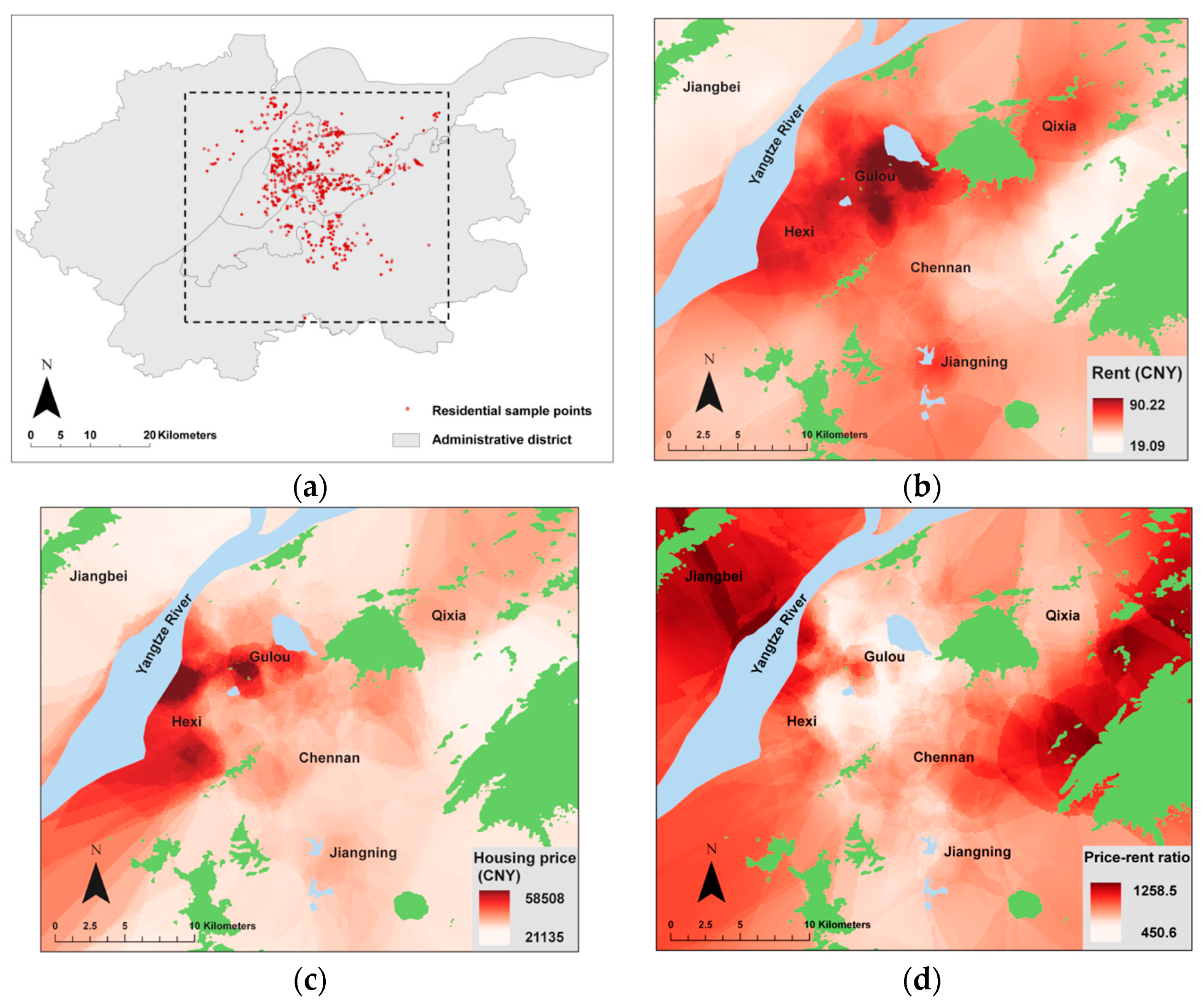
2.1. Study Area

This study was conducted in Nanjing, the second largest city in the Yangtze River Delta Urban Agglomeration [20]. Before 2002, the urban expansion of Nanjing had long been limited by its unique topographical conditions, which resulted in populations gathering in the old town. In 2002, Nanjing implemented a new urban planning policy, and three new towns were given more attention. Since then, the urban area of Nanjing has sprawled rapidly from the old town to the new towns. The study area covers all the main urban areas of Nanjing, which includes 10 districts. The rent samples in this area are regarded as belonging to the same residential market, and they accurately reflect the rent value in Nanjing.

2.2. Housing Data Collection and Processing

This article used residential data collected by the python crawler script from Lianjia (https://nj.lianjia.com), which is the largest real estate intermediary website in China. Housing data included the housing price, the housing rent, the area, the age, the address, the orientation, and the decoration condition of houses. Each house address was assigned by its unique latitude and longitude via the Google geocoding API (Application Programming Interface).

2.3. Process and Models

2.3.1. Spatial Autocorrelation Analysis

The extent of spatial dependency among the geographic entities was measured and analyzed in the spatial auto-correlation analysis. Spatial autocorrelation is the degree to which a geographic phenomenon of a regional unit or the value of an attribute is related to the same phenomenon or attribute value on an adjacent unit [21]. Spatial autocorrelation is divided into global spatial autocorrelation and local spatial autocorrelation. The global measurement mainly includes Moran’s I statistic, and the local spatial autocorrelation is measured by local Moran’s I index [5]. This paper used the global Moran index to determine whether the independent variable was a local variable or a global variable. The calculation formula is as follows:

$$I=\frac{{{\displaystyle \sum }}_{i=1}^n{{\displaystyle \sum }}_{j=1}^n{W}_{ij}{Z}_i{Z}_j}{{{\displaystyle \sum }}_{i=1}^n{{\displaystyle \sum }}_{j=1}^n{W}_{ij}{{\displaystyle \sum }}_{i=1}^n{Z}_i^2},$$

(1)

where I is the global Moran index value, i and j represent the two adjacent regions, Z_i and Z_j are the differences between the elements X_i and X_j and their mean X, respectively, and W_ij is the spatial weight, n is the total number of all elements, and W_ij is the spatial weight. When region i and region j have a common geographic boundary (regions i and j are adjacent), W_ij = 1; if region i and j are not adjacent, W_ij = 0.

2.3.2. Mixed Geographically Weighted Regression

The Mixed geographically weighted regression (MGWR) model is a combination of a common linear regression model and a geographically weighted regression model. Some parameters are set as constant parameters, and their corresponding variables are global variables, while some parameters are set as variable parameters, and their corresponding variables are local variables [22]. The parameter estimation uses a two-stage iterative method. The general form of the MGWR model is:

$$R_i={\displaystyle \sum }_{j=1}^n{\alpha }_j{X}_{ij}+{\beta }_0\left(ui,vi\right)+{\displaystyle \sum }_{j=n+1}^m{\beta }_j\left(ui,vi\right)X_{ij}+{\epsilon }_i,i=1,2,\cdot \cdot \cdot ,n,$$

(2)

where (ui, vi) is the spatial coordinate of the i sample point, j is the number of independent variables, α_j is the regression coefficient of the global variable, β_j is the regression coefficient of the local variable, and ε_i is the random disturbance term. R_i is the rent value of location i, X_ij represents the observation of the j independent variable at location i. Combined with the spatial weight matrix W(ui, vi), the regression parameter estimate at the i of the adjacent position can be expressed as:

$$\beta ={(X^{T}WX)}^{-1}{X}^{T}Wy.$$

(3)

In the geographically weighted regression model, the distance is used as a calculation index with a small weight. There are three kinds of spatial weight functions. Among them, the Gaussian function is the most commonly used algorithm [23], which is defined as:

$$W_i=\epsilon \left(\frac{d_i}{\sigma \theta }\right),$$

(4)

where ε the represents the standard normal distribution density; σ represents the standard deviation of the distance vector di; and θ is the bandwidth, whose value is determined by the cross validation (CV) principle. The cross-validation method is used to determine the bandwidth, and the CV test is used to confirm the optimal bandwidth of the GWR model [24]:

$$CV\left(h\right)=\frac{1}{n}{{\displaystyle \sum }}_{i=1}^n {(y_i{-\mathrm{y}}_{-\mathrm{i}}\left(h\right))}^2,$$

(5)

where h is the optimal bandwidth, which is the i point residential rent forecast value obtained by model fitting after the h bandwidth value is removed from the i point observation.

2.4. Spatial Distribution of Housing Rent, Price, and the Price–Rent Ratio

Figure 1a shows the spatial distribution of the rent sample points. The number of samples was 1621. The average residential rent ranged from 8.62 CNY/m² to 147.67 CNY/m², with a mean of 46.85 CNY/m². It was clearly found that the rent varied spatially in different areas (Figure 1b), whose distribution generally showed a multi-center cluster pattern. Specifically, the peak of rent was concentrated in Xinjiekou and Hexi, which are the main commercial centers of Nanjing (the Xinjiekou and Hexi areas are two important commercial centers in Nanjing and are densely distributed with many commercial facilities). There were also two sub-peaks in Dongshan and Xianlin. These regions are college towns, in which many colleges and universities are located. Meanwhile, the low rents were distributed in the southwest regions and southeast of the Yangtze River, where new towns are planned for Nanjing. From the characteristics of rent distribution, it can be seen that rent was closely related to the distribution of commercial centers and commercial facilities. Road networks and subway lines had a significant impact on the distribution of rent, especially the subway line.

The spatial distribution of housing prices in Nanjing was different from that of its rent (Figure 1c). A high-price cluster did not appear near Xinjiekou but appeared near the Hexi area and Wutai Mountain area, which include Nanjing’s key primary school and junior high school districts. In addition, the southern side of Xuanwu Lake was another high-priced area in Nanjing. High rents were also distributed around some institutions (including the Nanjing Foreign Language School, Beijing East Road Primary School, Southeast University, Chinese Academy of Sciences, and Nanjing Government) located in this area. Interestingly, the distribution of housing prices (the highest value was not in the city center) was different from that of the housing rent. This may be mainly because the residences with high housing prices are all school district houses (students in school district houses can enjoy compulsory education and enter the nearest school without exams). However, these “high-price” houses are distributed in an old town, meaning that the living environment of the residential communities is relatively poor, which keeps the rent relatively low.

The housing price–rent ratio (monthly housing rent per square meters divided by housing price per square meter) generally showed a decreasing trend from the urban fringe area to the urban center (Figure 1d). In the urban fringe area, the price–rent ratio of the Jiangbei area was mostly above 1000:1. Additionally, the price–rent ratio in the Wutai Mountain area, which is the most densely populated area in Nanjing, was also nearly 1200:1, because its house price increase greatly exceeds that of its rent, which leads to extremely high housing prices but low rent. Furthermore, other areas in the downtown area generally had a relatively low price–rent ratio, which ranged from 400:1 to 500:1. It is worth noting that the lowest price–rent ratio also reached 450:1, which is substantially higher than the normal value [25]. Thus, it can be concluded preliminarily that the housing prices in Nanjing show considerable capital bubbles.

From the spatial distribution of the housing rent, price, and price–rent ratio, we can summarize that commercial centers, schools, campuses, and subways may determine the housing utility value. Thus, the housing rent may be affected by these factors.

2.5. Selection of Explanatory Variables

Multiple complex influential factors could determine housing rent or price. These factors can be summarized based on three categories: macroeconomic factors, population, and house utility attributes. Initially, studies mainly focused on the inner correlation between housing price and house rent [26,27] and found a co-integration relationship between these two variables. Thus, some scholars have verified the impact of macroeconomic factors on housing prices [28,29,30]. Some studies found macroeconomic factors and demographic changes to be the most significant causes of rising housing prices in recent years [31,32,33].

Apart from macroeconomic factors, the utility of houses significantly influences their value [25,34]. From a household view, traffic conditions, neighborhood environments, and building structures are three key aspects to be concerned with. Traffic conditions are the first attribute that most buyers note. Numerous studies have been conducted to explore the relationship between traffic conditions and housing price. Among these, public transit [35], roads [36], and railways [37] are recognized as the key attributes. Neighborhood environment is also a significant attribute for houses. In addition, residents prefer to live proximate to open spaces [17,18], commercial centers [38], primary and middle schools [39], and universities [40]. Building structure, which refers to the internal attributes of a house’s structure, also play an important role in housing utility value. The decoration [9], orientation [7], age [39], and living area [8] can all determine the rent to a certain degree.

According to the spatial distribution of these three attributes (housing rent, price, and the price–rent ratio), as well as the existing relevant literature, we chose 13 indicators based on three aspects: neighborhood factors, traffic factors, and construction factors. Descriptions of the explanatory variables and their quantitative criteria are shown in

Table 1. Descriptions of the variables.

Category	Variable	Variable Type	Definition
Dependent Variable	Rent	continuous	Monthly rent per square meters
Neighborhood environment	Commercial Center	continuous	Network distance to the nearest commercial center 1 (meters)
	Supermarket	continuous	Network distance to the nearest supermarket (meters)
	School	continuous	Network distance to the nearest key public primary and middle school 2 (meters)
	College	continuous	Network distance to the nearest key university and college 3 (meters)
	Open Space	continuous	Network distance to the nearest urban park, green space, or square (meters)
	Hospital	continuous	Network distance to the nearest large hospital 4 (meters)
Traffic conditions	Subway	continuous	Network distance to the nearest subway station (meters)
	Expressway	continuous	Network distance to the nearest Expressway (meters)
	Railway	continuous	Network distance to the nearest Railway (meters)
Building structure	Area	continuous	Living Area (m2)
	Age	continuous	The age of the building: 2018 minus the actual built years
	Orientation	dummy	Orientation of the house (south = 2; Southeast, east, southwest = 1; others = 0)
	Decoration	dummy	Decoration of the house (furnished = 1; not furnished = 0)

¹ Commercial Center: The municipal-level Commercial Centers in Nanjing Commercial Network Planning (2015–2030). ² Key primary and middle school: The Top 20 primary or middle schools in Nanjing. ³ Key University and College: The universities or colleges based on the first batch of undergraduates. ⁴ large hospital: 3A level hospitals.

.

2.6. OLS Estimation of Explanatory Variables

We implemented a regression analysis of all explanatory variables using the OLS model. There are some variables worthy of attention in

Table 2. Regression result of the ordinary least square (OLS) model.

Variable	Std-Coefficient	T-Statistic	Sig.	VIF
Area	−0.199	0.000	0.000 *	1.237
Direction	−0.102	0.000	0.000 *	1.151
Decoration	0.181	0.000	0.000 *	1.071
Expressway	0.074	0.002	0.002 *	1.924
Railway	0.139	0.000	0.000 *	1.349
Subway	−0.191	0.000	0.000 *	1.508
Commercial Center	−0.413	0.000	0.000 *	4.215
School	−0.235	0.000	0.000 *	2.567
Supermarket	0.165	0.000	0.000 *	1.888
Age	−0.024	0.190	0.190	1.041
Open Space	−0.006	0.799	0.799	1.550
College	−0.284	0.000	0.000 *	1.600
Hospital	0.039	0.342	0.342	5.392
R2				0.512

Note: * represents a statistically significant probability at the 1% level.

. Firstly, except for hospitals, the variance inflation factors (VIFs) were smaller than five, which indicates that there was no redundancy between every explanatory variable. Secondly, an OLS analysis of the linear model was carried out. The R square of the linear model was 0.512, which shows that the model can explain 51.2% of the rent. Finally, the regression results show that at a significance level of 0.01, age, open spaces, colleges, and hospitals did not significantly relate to rent.

Before establishing the MGWR model, it was necessary to test whether the variables had significant spatial nonstationarity and determine whether the variables had spatial autocorrelation. The independent variables with nonspatial non-stationarity were regarded as global variables in the MGWR model.

Table 3. Spatial non-stationarity test.

Variable	Moran Index	Spatial Non-Stationarity
Area	0.272
Campus *	0.901	√
Commercial Center *	0.978	√
Decoration	0.086
Expressway *	0.835	√
Orientation	0.132
School *	0.967	√
Railway *	0.916	√
Subway *	0.739	√
Supermarket *	0.767	√

Note: * represents a statistically significant probability at the 1% level.

shows that the Moran indices of area, orientation, and decoration were less than 0.5. Thus, they were defined as global variables due to their insignificant spatial non-stationarity (under a 1% level). The other variables, which in the Moran index were all greater than 0.7, showed spatially significant spatial autocorrelation. Thus, commercial centers, primary and middle schools, colleges, subways, expressways, and railways were included in the local variables for calculation.

3. Results

3.1. Estimation of MGWR Model

The Gaussian function was applied to calculate the weights of MGWR. The optimal bandwidth of the local variable was determined by the CV verification method. MGWR results were compared with the traditional OLS model and the GWR model.

Table 4. Comparison between MGWR, GWR, and OLS model.

Models	AICc	R2	Adjusted R2	RMSE
OLS	13,102	0.512	0.508	302,889
GWR	12,682	0.634	0.619	224,667
MGWR	5331	0.724	0.689	78,943

Note: AICc—Akaike information criterion.

shows that the OLS model could only explain 51.2% of the total variance of the residential rent in Nanjing, and the sum of the squared residuals was 302,889. The MGWR model could explain 72.4% of the variance, which was 21.2% higher than the linear model and 9% higher than the GWR model. The Root Mean Squared Error (RMSE) of the MGWR model was much smaller than that of the OLS model and the GWR model, reflecting the superior metrics of the MGWR model. Therefore, the MGWR model was better than the OLS model and the GWR model in its fitting effect.

According to the local variable coefficient of the MGWR model (

Table 5. Regression coefficient local variable statistics.

Variable	Min	Quartile 1	Mean	Quartile 3	MAX
supermarket	−0.00233	−0.00059	0.00012	0.00074	0.00291
School *	−0.00278	−0.00198	−0.00124	−0.00087	0.00173
Commercial Center *	−0.00402	−0.00359	−0.00231	−0.00097	0.00102
Subway *	−0.00660	−0.00503	−0.00355	−0.00192	−0.00026
Expressway *	−0.00349	−0.00114	−0.00035	0.00044	0.00241
Railway *	0.00063	0.00141	0.00233	0.00328	0.00396
Campus *	−0.00436	−0.00157	−0.00110	−0.00040	0.00087

Note: * represents a statistically significant probability at the 1% level.

), the remaining local variables were significant at the 1% level, except that the supermarket variable did not pass the Monte Carlo test at the 1% level. Table 5 shows that the subway affected the rent most significantly. Railway was the only factor that had a positive mean coefficient in the local variables. The expressway had minimum mean coefficient. Next, commercial centers, primary and middle schools, universities and colleges, expressways, subway stations, and railways will be analyzed for their utility value to houses in Nanjing.

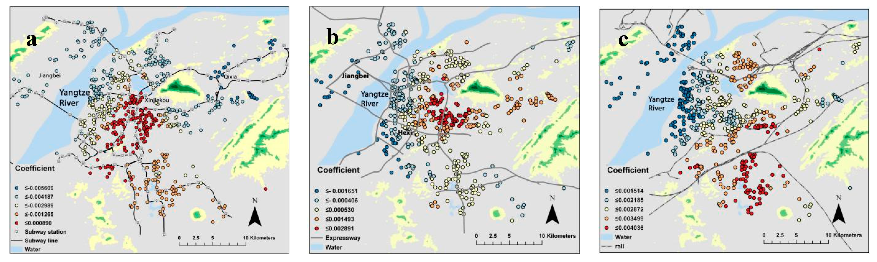
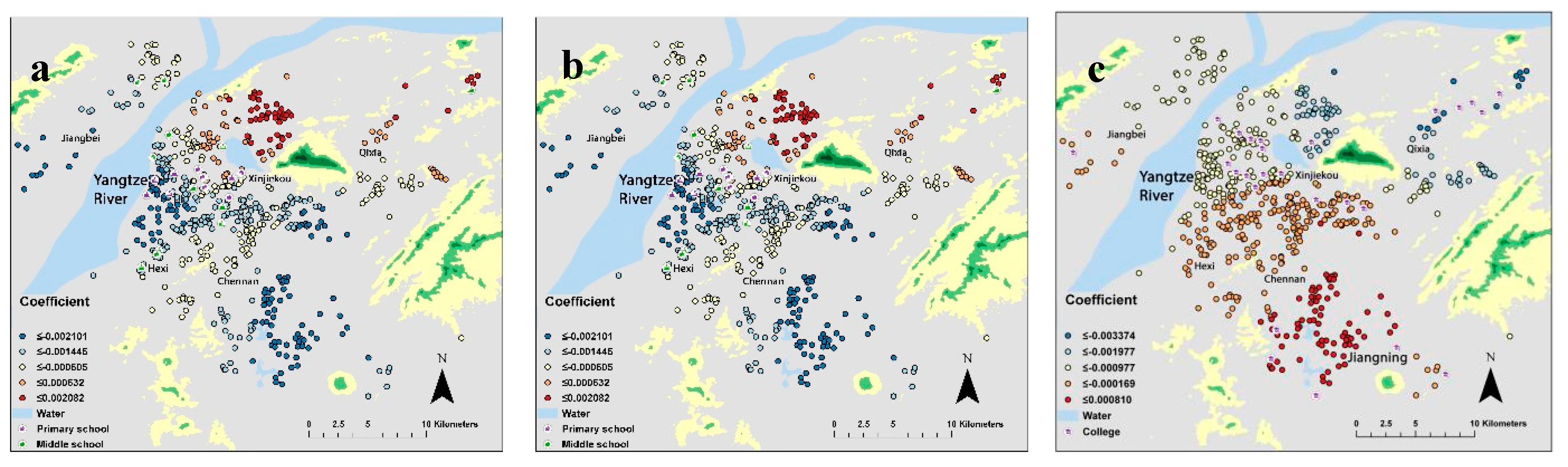
3.2. Local Variables Result

3.2.1. Traffic Conditions

Nanjing is a hilly city that crosses a river, and its complex terrain makes people more dependent on traffic facilities to commute. Thus, housing rents are determined by the traffic conditions in the individual locations. The mean coefficient of the expressway was the minimum of the six local variables, because almost half of the coefficients were positive, and half of the coefficients were negative (Figure 2a). The Yangtze River is a natural moat, blocking the passage of people on both sides of the river. Households on both sides of the Yangtze River have a higher demand for expressways. The coefficients of these areas were negative, in accordance with the actual circumstances. In addition, the houses in the Hexi and Jiangbei areas benefited most from the expressway in Nanjing. The reason for this result is that the road network in these two areas is sparse, as it is a new district of Nanjing, so the residents will depend more on the urban expressway for their daily commute. On the other hand, expressway construction in the new urban area is based on advanced planning, making the roads have a large retreated distance. On the other hand, the old expressways in the city center have a relatively small road retreat distance, which causes the peripheral houses to suffer from noise pollution. In Figure 3a, the houses in the city center are all “red”, which validates the previous assumption.

The construction of a subway tends to drive a sharp rise in housing prices and rents around the subway station. Figure 2b shows that the coefficient of the subway was also significant. The incremental effects of subways on rents in the urban edges were larger than those in the city center. Some houses in the center areas even show a negative coefficient for subways. The reason for this result is that there are already sufficient transportation facilities (e.g., bus lines, taxis, and public bicycles) in the city center, so residents are less dependent on the subway. For residents in the urban edges, the relatively scarce transportation facilities make subway systems the preferred mode of transport. Therefore, subway stations have a significant effect on the rise in rental prices in suburban areas.

Railway is another important mode of transportation for citizens. Some scholars have verified the negative impact of residential prices on the Beijing–Guangzhou railway line in terms of traffic noise and the division of urban internal traffic through the hedonic price model [8]. Figure 2c shows that the coefficients of the railway lines were different in different places, but all railway lines had a negative effect on housing rent. The differentiation law is as follows: the closer to the railway line, the lower the rent. One of the reasons for this result is the noise of the trains. At the same time, the railway line has a negative effect on the traffic division on both sides, which hinders the traffic of the surrounding regions. Therefore, the rent closer to a railway line was more strongly affected by the reduction of the railway line.

3.2.2. Neighborhood Environment

This paper selected four main commercial centers, which were individually located in Xinjiekou, Hexi, Chennan, and Jiangbei. Figure 3a shows that the coefficients for the commercial centers in most areas of the study were negative, indicating that the further away from the commercial center, the lower the rent. The maximum influence coefficient appeared near Xinjiekou, whose absolute value gradually decreased toward the southeast from the Drum Tower and the Confucius Temple area. The Jiangning and Qixia districts, which are far from downtown, were affected little by the commercial centers. The local residents tend to select local commercial facilities in these areas, so people less frequently consider the commercial centers when selecting their houses.

School district houses are the most important part of Chinese residential markets. The students in houses close to key primary and middle schools have priority to be enrolled in these schools. This paper selected the top 20 key primary and secondary schools. Figure 3b shows that most of these schools are located in the downtown. The coefficient of the key primary and middle schools in most areas of Nanjing was negative, that is, the closer to the school, the higher the rent. The northern area showed a positive coefficient. Therefore, we infer that people have a lower preference for primary and secondary schools when they select to rent northern houses in Nanjing.

Due to the numerous colleges and universities in Nanjing, many students need to rent apartments. Furthermore, university campuses in cities have another special attribute: they offer infrastructure services to surrounding residents (e.g., libraries, gyms, canteens, and classrooms). Figure 3c shows that the coefficients of universities and colleges were all negative. That is, colleges and universities increased rental prices for the surrounding houses. The houses in the Xianlin area had the largest coefficient in Nanjing. Thus, their value added to the surrounding rent is greater. The coefficient of the city center was small, while the Jiangning college town, which is located in the south of Nanjing, was the only area with a positive coefficient. The reason for this result is that the distribution of colleges and universities in the Jiangning District is relatively scattered, causing a low aggregation effect that produces less of an effect on the housing rent. On the other hand, the openness of campuses is relatively low in the Jiangning District because the college campuses are surrounded by walls. High isolation between the campus and the outside cut off internal and external links.

4. Conclusions

This article used the rents in Nanjing to spatially explore the utility value of houses from the perspective of rent. Our study shows that the distribution of housing rent generally has a multi-center group cluster pattern, which is not shared by the housing prices in Nanjing. The goal of this paper was to spatially explore the utility value of houses from the perspective of rent with the MGWR model. To identify the spatial non-stationarity and stationarity of variables, mixed geographically weighted regression was applied to deal with this problem. Area, orientation, and decoration did not show significant non-stationarity and were classified as global variables. Primary and middle schools, commercial centers, subways, expressways, railways, and colleges strongly affected rent, which influences significant degrees of spatial variation.

In terms of traffic conditions, subways affected the housing rent most strongly, especially in urban edge areas. Expressways showed diametrically opposite effects in some areas. Meanwhile, railway lines had an obvious value-reduced effect on surrounding houses. Therefore, how to balance the advantages and disadvantages of traffic facilities is an important issue in the future. Suburban areas should accelerate the construction of public transit and road networks. In the downtown area, road widening and noise reduction measures need to be accounted for.

In terms of the neighborhood environment, commercial centers showed a value-added effect to houses around the city center but had little effect on suburban houses. Schools and colleges are not the foremost considered objects for tenants, which is proven by the fact that that when a residential house has no school district attributes, the utility value of the house will decrease dramatically.

These results provide a reference for the management of the residential leasing market and the layout of urban infrastructure in Nanjing. Administrative departments may ponder the effects of each factor in the formation of urban planning. The factors that have a significant value-reduced effect on housing rent reflect the abundance of this infrastructure, and vice versa. Thus, the local residents’ living circumstances can be effectively ameliorated by improving the numbers and functionality of these infrastructures.

This study proves that the MGWR model is an effective residential utility value analysis method that is superior to the traditional OLS and GWR models. The MGWR model can identify non-stationary variables while controlling the smoothness of global variable parameters, making the results more accurate. However, there are still some limitations in this study. Social and economic factors also affect the housing rent to some extent at the micro scale in the main urban area of Nanjing. Future research should explore the relationship between residential houses and socio-economic attributes to more deeply understand the connotations of residential houses.

References

1. Niu, F.; Li, J. China Real Estate Development Market Report 2006; Social sciences academic press(CHINA): Beijing, China, 2007. [Google Scholar]
2. Niu, F.; Li, J. China real Estate Development Market Report 2018; Social sciences academic press(CHINA): Beijing, China, 2019. [Google Scholar]
3. China PBC & CCDC: Treasury Bond and Other Bond Yield: Daily. Available online: https://www.ceicdata.com/en/china/pbc--ccdc-treasury-bond-and-other-bond-yield-daily (accessed on 22 August 2019).
4. De Mare, G.; Manganelli, B.; Nesticò, A. Dynamic Analysis of the Property Market in the City of Avellino (Italy)—The Wheaton-Di Pasquale Model Applied to the Residential Segment; Murgante, B., Misra, S., Carlini, M., Torre, C., Nguyen, H.Q., Taniar, D., Apduhan, B.O., Gervasi, O., Eds.; Lecture Notes in Computer Science LNCS; Springer: Berlin/Heidelberg, Germany, 2013; Volume 7973, pp. 509–523. [Google Scholar]
5. Qing, T.; Wei, X.; Fu, A. A GWR-Based Study on Spatial Patter and Structurals Housing Price Deter minants of Shanghai. Econ. Geogr. 2012, 32, 52–58. [Google Scholar]
6. Geniaux, G.; Martinetti, D. A new method for dealing simultaneously with spatial autocorrelation and spatial heterogeneity in regression models. Reg. Sci. Urban Econ. 2016, 72, 74–85. [Google Scholar] [CrossRef]
7. Zou, Y. Analysis of spatial autocorrelation in higher-priced mortgages: Evidence from Philadelphia and Chicago. Cities 2014, 40, 1–10. [Google Scholar] [CrossRef]
8. Li, H.; Wei, Y.D.; Wu, Y.; Tian, G. Analyzing housing prices in Shanghai with open data: Amenity, accessibility and urban structure. Cities 2019, 91, 165–179. [Google Scholar] [CrossRef]
9. Lu, J. The value of a south-facing orientation: A hedonic pricing analysis of the Shanghai housing market. Habitat Int. 2018, 81, 24–32. [Google Scholar] [CrossRef]
10. Huang, Z.; Chen, R.; Xu, D.; Zhou, W. Spatial and hedonic analysis of housing prices in Shanghai. Habitat Int. 2017, 67, 69–78. [Google Scholar] [CrossRef]
11. Rosen, S.; Journal, T.; Feb, N.J.; Rosen, S. Hedonic Prices and Implicit Markets: Product Differentiation in Pure Competition. J. Political Econ. 1974, 82, 34–55. [Google Scholar] [CrossRef]
12. Gao, J.; Li, S. Detecting spatially non-stationary and scale-dependent relationships between urban landscape fragmentation and related factors using Geographically Weighted Regression. Appl. Geogr. 2011, 31, 292–302. [Google Scholar] [CrossRef]
13. O’Sullivan, D. Geographically Weighted Regression: The Analysis of Spatially Varying Relationships (review). Geogr. Anal. 2003, 35, 272–275. [Google Scholar] [CrossRef]
14. Brunsdon, C.; Fotheringham, A.S.; Charlton, M. Geographically weighted summary statistics—A framework for localised exploratory data analysis. Comput. Environ. Urban Syst. 2002, 26, 501–524. [Google Scholar] [CrossRef]
15. Helbich, M.; Brunauer, W. Mixed Geographically Weighted Regression for Hedonic House Price Modelling in Austria; Univerity of Heidelberg: Heidelberg, Germany, 2010; Available online: https://www.geog.uni-heidelberg.de/md/chemgeo/geog/gis/helbich_brunauer_giforum2010.pdf (accessed on 29 September 2019).
16. Liang, X.; Liu, Y.; Qiu, T.; Jing, Y.; Fang, F. The effects of locational factors on the housing prices of residential communities: The case of Ningbo China. Habitat Int. 2018, 81, 1–11. [Google Scholar] [CrossRef]
17. Qin, Z.; Yu, Y.; Liu, D. The Effect of HOPSCA on Residential Property Values: Exploratory Findings from Wuhan, China. Sustainability 2019, 11, 471. [Google Scholar] [CrossRef]
18. Liebelt, V.; Bartke, S.; Schwarz, N. Urban Green Spaces and Housing Prices: An Alternative Perspective. Sustainability 2019, 11, 3707. [Google Scholar] [CrossRef]
19. Yang, Y.; Liu, J.; Xu, S.; Zhao, Y. An Extended Semi-Supervised Regression Approach with Co-Training and Geographical Weighted Regression: A Case Study of Housing Prices in Beijing. ISPRS Int. J. Geo-Inf. 2016, 5, 4. [Google Scholar] [CrossRef]
20. Development Planning of Urban Agglomeration in Yangtze River Delta. Available online: http://www.ndrc.gov.cn/zcfb/zcfbghwb/201606/t20160603_806390.html (accessed on 22 August 2019).
21. Baumont, C.; Ertur, C.; Le Gallo, J. Spatial Analysis of Employment and Population Density: The Case of the Agglomeration of Dijon 1999. Geogr. Anal. 2003, 36, 146–176. [Google Scholar] [CrossRef]
22. Brunsdon, C.; Fotheringham, A.; Charlton, M. Some Notes on Parametric Significance Test for Geographically Weighted Regression. J. Reg. Sci. 1999, 39, 497–524. [Google Scholar] [CrossRef]
23. Waltert, F.; Schläpfer, F. Landscape amenities and local development: A review of migration, regional economic and hedonic pricing studies. Ecol. Econ. 2010, 70, 141–152. [Google Scholar] [CrossRef] [Green Version]
24. Farber, S.; Páez, A. A systematic investigation of cross-validation in GWR model estimation: Empirical analysis and Monte Carlo simulations. J. Geogr. Syst. 2007, 9, 371–396. [Google Scholar] [CrossRef]
25. Chen, A. China’s Urban Housing Reform: Price-rent ratio and Market Equilibrium. Urban Stud. 1996, 33, 1077–1092. [Google Scholar] [CrossRef]
26. Ozanne, L.; Thibodeau, T. Explaining metropolitan housing price differences. J. Urban Econ. 1983, 13, 51–66. [Google Scholar] [CrossRef]
27. Shiller, R.; Case, K. Forecasting Prices and Excess Returns in the Housing Market. Real Estate Econ. 1990, 18, 253–273. [Google Scholar] [Green Version]
28. Potepan, M.J. Explaining Intermetropolitan Variation in Housing Prices, Rents and Land Prices. Real Estate Econ. 1996, 24, 219–245. [Google Scholar] [CrossRef]
29. Wheaton, W. Real Estate “Cycles”: Some Fundamentals. Real Estate Econ. 1999, 27, 209–230. [Google Scholar] [CrossRef]
30. Quigley, J. Real Estate Prices and Economic Cycles. Int. Real Estate Rev. 1999, 2, 1–20. [Google Scholar]
31. Aoki, K.; Proudman, J.; Vlieghe, G. House Prices, Consumption, and Monetary Policy: A Financial Accelerator Approach. J. Financ. Intermed. 2002, 13, 414–435. [Google Scholar] [CrossRef]
32. Bernanke, B.; Gertler, M. Monetary Policy and Asset Price Volatility. Econ. Rev. 1999, 84, 17–51. [Google Scholar]
33. Bencardino, M.; Nesticò, A. Demographic changes and real estate values. A quantitative model for analyzing theur ban-rurallinkages. Sustainability 2017, 9, 536. [Google Scholar] [CrossRef]
34. Marks, D. The Effect of Rent Control on the Price of Rental Housing: An Hedonic Approach. Land Econ. 1984, 60, 61–94. [Google Scholar] [CrossRef]
35. Zhang, X.; Liu, X.; Hang, J.; Yao, D.; Shi, G. Do urban rail transit facilities affect housing prices? Evidence from China. Sustainability 2016, 8, 380. [Google Scholar] [CrossRef]
36. Guang, T.; Wei, Y.H.D.; Li, H. Effects of accessibility and environmental health risk on housing prices: A case of Salt Lake County, Utah. Appl. Geogr. 2017, 89, 12–21. [Google Scholar]
37. Blanco, J.C.; Flindell, I.H. Property Prices in Urban Areas Affected by Road Traffic Noise. Appl. Acoust. 2011, 72, 133–141. [Google Scholar] [CrossRef]
38. Wang, A.; Lin, L.; Bao, S.J. Spatially Non-stationary Analysis Between Commercial Land Price and Driving Factors in Hefei City. Sci. Geogr. Sin. 2017, 37, 1535–1545. [Google Scholar]
39. Xu, Y.; Song, W.; Liu, C. Social-spatial accessibility to urban educational resources under the school district system: A case study of public primary schools in Nanjing, China. Sustainability 2018, 10, 2305. [Google Scholar] [CrossRef]
40. Won, J.; Lee, J.S. Investigating how the rents of small urban houses are determined: Using spatial hedonic modeling for Urban Residential Housing in Seoul. Sustainability 2018, 10, 31. [Google Scholar] [CrossRef]
Figure 1. The spatial distribution of (a) sample points; (b) housing rent; (c) housing price; (d) the housing price–rent ratio.
Ijgi 08 00431 g001
Figure 2. The spatial distribution of coefficients: (a) subway; (b) expressway; (c) railway line.
Ijgi 08 00431 g002
Figure 3. The spatial distribution of coefficients: (a) commercial centers; (b) primary and middle schools; (c) colleges and universities.
Ijgi 08 00431 g003