A Reconstruction Method for Broken Contour Lines Based on Similar Contours

Abstract

The reconstruction of a broken contour line is a prerequisite for the automated processing of contour lines. When the situation with broken contour lines is severe or the terrain is more complex, incorrect and missing connections are most likely to occur using traditional methods. In this paper, a reconstruction method for broken contour lines based on similar and completely closed contours is proposed. First, node densification is conducted on broken contour lines to improve the identification accuracy of the reference line. Second, the discrete Fréchet distance is used to select a reference line and perform reconstruction. Finally, the actual data of Yunnan Province are utilized for verification. The results show that the method proposed in this paper can achieve better reconstruction of broken contour lines, especially for severe broken contour situations or complex terrains; the reconstruction accuracy is significantly improved over that of the traditional method, indicating good feasibility.

1. Introduction

Contour lines are an important element in topographic maps and one of the main data sources for constructing digital elevation models (DEMs), which are 3D models. When extracting contour lines from topographic maps, inevitably, gaps may occur because other features in topographic maps can overlay and cross the contour lines. Gaps cause problems for the generation of DEMs and the construction of 3D simulations [1]. The reconstruction of broken contour lines can be realized to form a complete contour line by identifying the degree of matching among broken lines in terms of geometry (e.g., angles and directions), which is known as breakpoint connection. In recent years, scholars have conducted a large number of studies on the reconstruction of broken contour lines. According to the reconstruction form for connecting breaking points, the reconstruction of broken contour lines can be divided into three categories: adjacency-relationship-based [2,3], continuity-based [1,4,5], and gradient-vector-flow-based [6,7,8] reconstruction. This paper focuses on the continuity-based reconstruction of broken contour lines.

The continuity-based reconstruction method, which includes both the geometric and topological characteristics of a contour line, is concise and easy to implement, making it the most commonly used reconstruction method; it completes breakpoint matching and curve reconstruction by identifying the continuity of contour breakpoints via geometric and topological characteristics. Among the various methods, Arrighi et al. [9] proposed the minimum point pair method, which realizes breakpoint connection based on the principle of the minimum breakpoint distance or the minimum directional difference. Samet et al. [4,5] optimized the minimum point pair method to refine the constraint criterion for breakpoint matching and used Newton’s difference interpolation algorithm to complete the matching connection of a breakpoint. Gul et al. [3] proposed a breakpoint extension and intersection identification matching method that determines the directions of all broken lines in a region using the distances and direction angles of breakpoints and completes the breakpoint connection where the broken lines intersect. Most reconstruction methods for broken contour lines based on continuity only consider the characteristics of broken contour lines for connection using the Euclidean distance of the interbreakpoint to assist in the reconstruction of breakpoints or azimuthal lines. In the case of a small breakpoint distance and small curvature changes, the reconstruction effect is better. In the case of a large breakpoint distance or large curvature changes, such as saddle-shaped terrain, existing methods have difficulty effectively judging the original trends of broken lines and are prone to incorrect and missing breakpoint connections. Therefore, a reconstruction method for broken contour lines based on a reference line is proposed using similarity to measure the Fréchet distance, and two contour lines with high similarity around the broken contour line are selected as fixed reference lines to assist in the reconstruction of broken contour lines.

This paper is organized as follows. Section 1 analyzes the shortcomings of the existing continuity-based reconstruction method for broken contour lines and proposes an improved idea of a similarity measurement based on the Fréchet distance. Section 2 elaborates on the reconstruction method for broken contour lines based on a reference line. Section 3 describes the actual data experiment and analysis. Section 4 presents the discussion and research conclusions of this work.

2. Relevant Works

2.1. Continuity-Based Reconstruction Method of Contour Lines

For the continuity-based method, the Euclidean distance is typically directly used to identify the minimum distance between the breakpoints of a connection to realize the reconstruction of the broken contour line. The Euclidean distance is one of the most commonly used methods for spatial measurements and is applied to describe the real distance between two points in m-dimensional space. If there are two points on the two-dimensional plane (i.e., $p_i(x_i,y_i)$ and $p_j(x_j,y_j)$), then the Euclidean distance between these two points is calculated as follows:

$$d\left(p_i,p_j\right)={\sqrt{{\left(x_i-x_j\right)}^2+{\left(y_j-y_i\right)}^2}}^{}.$$

(1)

The Euclidean distance can be used to calculate the distance relationship between two breakpoints for the reconstruction of a contour line, and a classic method to accomplish this is the minimum point pair method. As shown in Figure 1, breakpoints A, B, C, and D belong to four broken contour lines (1, 2, 3, and 4, respectively), where the Euclidean distance is used to measure and calculate the minimum distances between each breakpoint and its adjacent contour line. Among them, the minimum distance between breakpoint A and the other breakpoints is calculated as Dmin (A, X) to yield X = B for the connection of breakpoints A and B for the reconstruction of broken contour lines 1 and 2 into a complete contour line. Similarly, breakpoints C and D are connected to reconstruct broken contour lines 3 and 4 into a complete contour line.

However, the reconstructed line created with this method is usually a straight line, and when the contour line is complex, the reconstructed line is prone to cross dislocation. For this reason, some scholars have put forward a method to add direction for auxiliary identification (based on the extraction of the interbreakpoint Euclidean distance) and a direction angle [3]; the search window is set to calculate the directions of all breakpoints in the window, which allows the appointed breakpoint and alternative breakpoint in the neighborhood search window to extend in each direction. If the extension lines intersect, the breakpoints are matched and connected; the effect is shown in Figure 2.

2.2. Limitations in Existing Methods

The method for the reconstruction of broken contour lines is easy to implement by using the Euclidean distance with an auxiliary direction, making it suitable for the reconstruction of contour lines with a better surface effect, smaller breakpoint distance, and flatter terrain, as shown in Figure 3 A. However, when the following cases occur due to only considering the individual characteristics of a broken contour line for connection, it is difficult to accurately determine the original trend of the broken contour line, making it prone to incorrect and missing connections.

(1)

The overall breaking of a contour line is severe, and only a small part of the break remains, as shown in Figure 3 B;

(2)

The topography of the broken contour line area is complex (e.g., ridges, valleys, and saddles), as shown in Figure 3 C.

According to the above two cases, some scholars have put forward the strategy of using breakpoint classification and directional differences for the reconstruction of broken contour lines [10] to enhance the connection effect of a long, broken contour line on flat terrain. However, with the increase in complex breaks, cross dislocation and the number of missing connections greatly increase [11], which leads to a large workload, including artificial checks and corrections, and the practicality of the method decreases rapidly.

2.3. Improved Idea via the Introduction of Fréchet Distance

According to the above problem, a reconstruction method for broken contour lines based on a reference line is proposed using similarity to measure the Fréchet distance. Two contour lines with high similarity around a broken contour line are selected as the reconstruction reference to realize the node densification of the breakpoint and the reconstruction of the contour line under long-distance breaks and complex terrain environments.

Linear elements, such as contour lines, can be regarded as a set of spatial points, where the geometric similarity is regarded as the similarity of the spatial point set [12]. The Hausdorff distance [13] and Fréchet distance [14] are commonly used to measure the similarity of a spatial point set, where the Fréchet distance is typically used to judge the similarity between two consecutive curves [15,16,17]. The Fréchet distance includes a continuous Fréchet distance and a discrete Fréchet distance. Because the points in the actual contour line are discretized, the similarity between contour lines is determined by using the discrete Fréchet distance. The discrete Fréchet distance d_F is defined as follows [18]:

① Given a polygonal chain $P=\langle p_1,p_2,\dots ,p_n\rangle$ with n vertices and a k step along P, the vertices of P are segmented into k nonintersecting, nonempty subsets, ${\left\{P_i\right\}}_{i=1,\dots ,k}\left(1\le k\le n\right)$, which results in $P_i=\langle p_{n_{i-1}+1},\dots ,p_{n_i}\rangle$ and $0=n_0<n_1<\dots <n_k=n$.

② Given two polygonal chains $A=\langle a_1,a_2,\dots ,a_m\rangle$ and $B=\langle b_1,b_2,\dots ,b_n\rangle$, the combination step along A and B is equal to a k step along A ${\left\{A_i\right\}}_{i=1,\dots ,k}$ and a k step along B ${\left\{B_i\right\}}_{i=1,\dots ,k}$; therefore, $1\le i\le k$, where $|A_i|=1$ or $|B_i|=1$ (indicating that $A_i$,$B_i$ has an exact vertex).

③ The calculation of a combination step along chains A and B, $W=\{\left(A_i,B_i\right)\}$, is shown below.

$$d_F^W=\underset{i}{\max }\underset{(a,b)\in A_i\times B_i}{\max }d\mathrm{is}(a,b)$$

(2)

Thus, the discrete Fréchet distance between chains A and B is shown below.

$$d_F(A,B)=\begin{array}{cc}\underset{W}{\min }& d_F^W(A,B)\end{array}$$

(3)

3. The Reconstruction of Broken Contour Lines Based on a Reference Line

In this paper, the foundation for the proposed reconstruction method for broken contour lines based on a reference line consists of three parts: (1) contour line node densification (to improve the identification accuracy of the reference line similarity), (2) the Fréchet distance (for the selection of a reference line), and (3) the interpolation and connection of a broken contour line based on the selected reference line (to complete the reconstruction of a contour line).

3.1. Contour Line Node Densification

When using the discrete Fréchet distance to measure contour similarity, if the distance between some contour nodes is too large, the points are relatively sparse and the difference compared to the continuous Fréchet distance is large during the calculation, which makes it difficult to accurately measure the similarity. As shown in Figure 4a, there are two lines (line abcd and line ef), and the continuous Fréchet distance between them should be d(b,v), which is the distance from point b to line ef (i.e., the distance represented by the dashed line in Figure 4a).

Due to the sparse nodes in line ef, the calculated discrete Fréchet distance is d(b, e) (i.e., the length of the dotted line in Figure 4a), which is much greater than the real continuous Fréchet distance. Therefore, to make the discrete Fréchet distance closer to the continuous Fréchet distance, node densification is required for line ef in Figure 4a to obtain line eghijf in Figure 4b. Then, the densified, discrete Fréchet distance d(b, h), which is the length of the dotted line in Figure 4b, is closer to the continuous Fréchet distance than the original discrete Fréchet distance d(b, e), resulting in accurate similarity identification between the two lines. The densification algorithm is performed as follows:

Step 1: The distance between two adjacent nodes is calculated from the first node of a contour line.

Step 2: If the distance d does not exceed the threshold, no processing is required. If the threshold is exceeded, m points are uniformly inserted, where the formula for m is as follows:

$$m=\lfloor \frac{d}{t}\rfloor +1.$$

(4)

In Equation (4), d represents the distance between two nodes, and t represents the threshold, which is usually the median of all distances for any two connective nodes in the original contour lines. The symbol ⎣ ⎦ denotes the floor function, which rounds down integers.

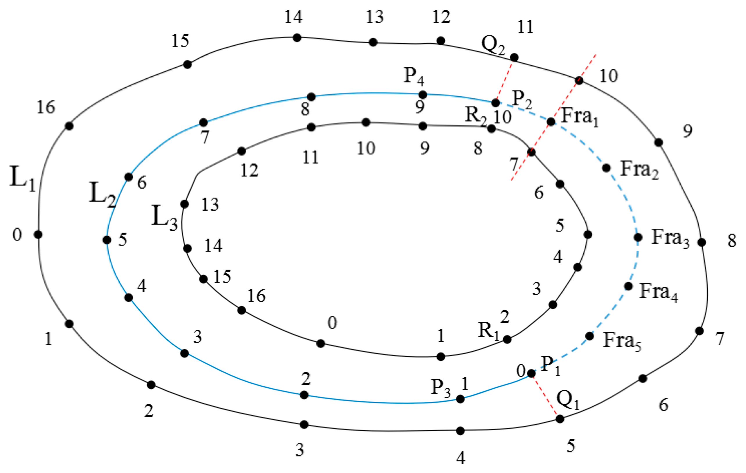
3.2. Reference Line Selection Based on the Fréchet Distance

The reference line refers to a complete contour line which is located around the broken contour line and has a consistent trend. In the case of broken contour lines with a small distance between them and simple topography, it is easy to identify the reference line using the discrete Fréchet distance. However, when the situation of the broken contour lines is complicated or the terrain is complex, it is easy to use all of the broken contour lines to identify the similarity and misjudge the reference line. Therefore, in this paper, points along the broken contour line are gradually selected first; then, the Fréchet distance between the points and closed contours surrounding the contour lines is calculated. Finally, the reference line can be identified by similarity identification. During the selection process, to avoid inaccurate similarity identification caused by the short length of the selected points, the length between the selected points can be restricted by the empirical threshold; if the length is excessively short, points can be added to reach the length for similarity identification. Figure 6 illustrates the specific steps for selecting the reference line:

Step 1: According to the spatial inclusion relation, the adjacent closed contour which can be used as the reference line of the broken contour line is selected. As shown in Figure 5, there are three contour lines (L₁, L₂, and L₃) surrounding the broken contour line L₄. Since L₁ contains L₄, L₁ is regarded as the reference line of L₄.

Step 2: Taking the breakpoints of the fracture contour as a starting point, some points on the broken contour line are selected, and the similarity between the points and adjacent contours is judged. As shown in Figure 5, the breakpoint on one side of L₄ is d₁; first, the nearest points (b₁ and c₁) are calculated from d₁ to the adjacent closed contour lines (L₂ and L₃). By picking the point d₂ on L₄ by using an empirical length threshold l, the nearest points b₂ and c₂ are also calculated from d₂ to L₂ and L₃. If the length between b₁ and b₂ or c₁ and c₂ is smaller than the empirical threshold, then b₂ or c₂ is removed; then, the point d₃ on L₄ is used to capture the nearest point from d₃ to L₂ and L₃ until the nearest points along L₂ and L₃ satisfy the empirical threshold. As shown in Figure 6, when d₅ is obtained on L₄, the point c₂ that satisfies the empirical threshold is captured on L₃.

Step 3: The discrete Fréchet distances between the broken contour line and the completely closed surrounding contour lines are each calculated. The contour line with the minimum Fréchet distance is taken as the reference line. As shown in Figure 5, by using Equations (2) and (3), the discrete Fréchet distances d_F(d₁,b₁) and d_F(d₁,c₁), which are from d₁d₅ to b₁b₄ and c₁c₂, respectively, are each calculated, and the discrete Fréchet distances d_F(d₆,b₅) and d_F(d₁₀,c₄) that are from d₆d₁₀ to b₅b₈ and c₃c₄, respectively, are also calculated. Since d_F(d₁,b₁) < d_F(d₁,c₁) and d_F(d₆,b₅) < d_F(d₁₀,c₄), d₁d₅ to b₁b₄ and d₆d₁₀ to b₅b₈ are more similar. Additionally, because b₁b₄ and b₅b₈ both belong to L₂, L₂ is chosen as the reference line for L₄. If the selection line in this step does not belong to the same completely closed contour line, then Steps 2 and 3 should be repeated until the closed reference line is found.

3.3. Broken Contour Line Interpolation and Connection Based on the Reference Line

According to the reference contour line obtained in Section 2.2, the broken contour line can be interpolated and connected. The basic idea is to determine the projected position of the broken contour line in the reference contour line to identify the extended direction of the reference contour line. Then, according to the projected position, extended direction, and elevation information, the interpolated points and connection order of the broken contour line are determined and, eventually, all interpolation points are connected to reconstruct the broken contour lines. Figure 6 is shown as an example to illustrate the specific steps.

Step 1: The projected position of a reference contour line is determined. In Figure 6, suppose that the points on the broken contour line L₂ and its two reference lines (L₁ and L₃) all have serial numbers. Broken contour line L₂ has two breakpoints, P₁ and P₂, which correspond to the first and last nodes of the broken line, respectively. Two points, Q₁ and Q₂, are projected onto the reference contour line L₁. If Q₁ and Q₂ already exist on the reference contour line L₁, the serial numbers of Q₁ and Q₂ on the completely external contour line are directly calculated. If either Q₁ or Q₂ (or neither) is on the reference contour line L₁, the point is inserted into the corresponding position to calculate the serial number of the inserted point on the contour line L₁. Thus, the projected serial numbers for P₁ and P₂ on the reference contour line L₁ are equal to those of Q_i1 and Q_i2, respectively. In Figure 6, the serial numbers for Q_i1 and Q_i2 are 5 and 11, respectively. Similarly, the serial number of the projected point on the reference contour line L₃ is obtained.

Step 2: The interpolation sequence at the breakpoint is determined. The adjacent points (P₃ and P₄) of the breakpoints (P₁ and P₂) on the broken contour line L₂ are used to calculate the projected points (Q_i3 and Q_i4) on the reference contour line L₁. If Q_i1 < Q_i3, Q_i2 > Q_i4, and Q_i1 > Q_i2, which indicates that the serial number 0 of the projection points from L₂ to L₁ do not exist, then L₂ has the same serial sequence as L₁. The values on L₁ projected by the subsequently densified interpolation values of L₂ are sequenced as Q_i2, Q_i2+1, ..., Q_i1-1, and Q_i1. Conversely, if Q_i1 > Q_i3, Q_i2 < Q_i4, and Q_i1 < Q_i2, then the serial number 0 of the projection points from L₂ to L₁ exist, and L₂ has the opposite serial sequence to L₁. The values on L₁ projected by the subsequently densified interpolation values of L₂ are sequenced as Q_i2, Q_i2+1, ..., Q_i1-1, and Q_i1. As shown in Figure 6, Q_i1 is equal to 5, Q_i2 is equal to 11, Q_i3 is equal to 4, and Q_i4 is equal to 12, which conforms to the reverse order rule; therefore, the interpolation sequence is identified as Q_i2, Q_i2-1, …, Q_i1+1, and Q_i1, which is equal to 11, 10, 9, 8, 7, 6, and 5 on L₁. Likewise, the corresponding interpolation sequence on L₃ can be derived.

Step 3: According to the interpolation order in the breakpoint location, the nodes are successively densified at the breakpoint location, and the densified points are connected to achieve contour line reconstruction. According to Step 1, the projected points of breakpoints P₁ and P₂ on the broken contour line L₂ using the reference contour lines L₁ and L₃, respectively, are obtained (i.e., Q₁ and Q₂ for R₁ and R₂, respectively). According to Step 2, the interpolated values of the densified points on the broken contour line are obtained in the sequence as 11, 10, 6, 5. Starting from Q₂ and R₂, the next nodes on the reference contour lines L₁ and L₃ are calculated in the order corresponding to the interpolated point coordinates for the broken contour line L₂. The calculation formula is shown below:

$$T=\frac{|H_{L2}-H_{L1}|}{|H_{L3}-H_{L1}|}$$

(5)

$$X_{Fran}=X_{Qn}+T(X_{Rn}-X_{Qn})$$

(6)

$$Y_{Fran}=Y_{Qn}+T(Y_{Rn}-Y_{Qn})$$

(7)

where T represents the proportion of contour line interpolation; H_L2 represents the elevation value of the current broken contour line; and $H$_L1 and H_L3 represent the elevation values of the reference contour lines L₁ and L₃, respectively. X_Pn and Y_Pn represent the x and y coordinates of the interpolated point P_n at the breakpoint, respectively; these values translate into (X_Qn, Y_Qn) and (X_Rn, Y_Rn), which represent the x and y coordinates of the corresponding sequence points on the reference contour lines L₁ and L₃, respectively.

As shown in Figure 6, according to the above equation, the x and y coordinates of the interpolated point Fra₁ at the corresponding points 10 and 7 on the reference lines L₁ and L₃, respectively, are calculated based on the interpolation sequence at the breakpoint. After successive calculations, the positions of the interpolation points (Fra₁ to Fra₅) on all contour lines are obtained via sequential connection for contour line reconstruction.

4. Experiment and Results

4.1. Experimental Data and Environment

Based on the WJ-III map workstation developed by the Chinese Academy of Surveying and Mapping, the reconstruction method for broken contour lines based on a reference line was embedded using OpenMP into the C++ environment for the reconstruction of broken contour lines. The universality and accuracy of this method is verified in this paper. In this experiment, broken contour line data within a certain area of Yunnan (with a total area of 29.1 km²) were taken as examples, as shown in Figure 8a. This area has terrain that is mainly mountainous and hilly, with a total of 5948 contour lines and a basic contour line interval of 5 m, including 3277 broken contour lines; the number of breaks accounts for 55% of the total, and the total reconstruction time was 328 s. According to the situation of the broken contour line, the broken contour line can be divided into two cases connecting the breakpoint directly: if the connecting line intersects with other contour lines, the broken contour line is called a complex fracture; otherwise, it is called a general fracture. The experiment environment was a Microsoft Windows 7 64-bit operating system, the central processing unit (CPU) was an Intel Core 7-6700, the main frequency was 3.40 GHz, and the memory (RAM) was 4 GB in size.

4.2. Universality Analysis

4.2.1. Reference Line Selection

Due to the dense contour line in the experimental area, which is the most intensive and broken line in the experimental area, to reduce the number of calculations and improve the calculation accuracy, the index curve around the broken contour line was taken first as the reference line for reconstruction. Based on the Fréchet distance, the reference line for the broken contour line can be directly calculated. However, due to the surroundings of some broken contour lines lacking two complete index curves as reference lines, the original closed contour line and the adjacent contour line were taken as the reference lines for supplementary reconstruction in this experiment. Figure 7a shows that for the contour line break in the black box, because there is only a complete index curve externally, no reconstruction was performed in the first step; in the second step, the original closed contour line and the adjacent contour line were taken as the reference lines for reconstruction. Here, reference lines exist on both sides of the broken contour line to achieve a complete connection, and the result is shown in Figure 7b.

4.2.2. Contour Line Reconstruction

Figure 8a shows the overall result after the reconstruction of broken contour lines in the experimental area by using the method in this paper, where the red line represents the reference line, the blue line represents the broken contour line, and the purple line represents the reconstructed contour line. Statistics on the reconstructed contour lines are shown in

Table 1. Statistics on the reconstructed broken contour lines in the experimental area.

No	Statistical Item	Statistical Result
1	Total number of contour lines	5948
2	Total number of broken contour lines	3277
3	Proportion of breaks	55%
4	The number of general broken contour lines	1246
5	The number of complex broken contour lines	2031
6	Correct reconstruction of broken contour lines	3064
7	Correct reconstruction of general broken contour lines	1225
8	Correct reconstruction of complex broken contour lines	1839
9	Reconstruction accuracy rate of the broken contour lines	93.5%

. The correct criterion is that the broken contours are closed and do not intersect with the other contours. The results show that the method in this paper can effectively reconstruct both general and complex broken contour lines. The reconstruction accuracy of the broken contour lines was 93.5%, with an overall favorable effect for the reconstruction of broken contour lines.

To further verify the effect of the reconstruction of complex broken contour lines, the corresponding typical areas were selected for local amplification in this paper. In severe cases of broken contour lines, only a small number of breaks (before reconstruction in Figure 8b and after reconstruction in Figure 8c and Figure 9) and complex terrain with broken contour lines (before reconstruction in Figure 8d and after reconstruction in Figure 8e and Figure 10) remain; the proposed method in this paper can better realize the reconstruction of broken contour lines.

4.3. Superiority Analysis

To further illustrate the superiority of the method in this paper, the minimum point pair method and the method presented in this paper were used to carry out an experiment on reconstructed broken contour lines under the same conditions. The results are shown in Figure 11.

(1) General Broken Contour Lines

By using the Delaunay triangulation method [19] and Equation (8), the distance between contours that were reconstructed is statistically significant. The results are shown in

Table 2. Statistics of the distances of the reconstructed contours (unit: meter), where SD indicates the standard deviation.

Method	1–2	2–3	3–4	4–5	5–6	SD	6–7	7–8	8–9	9–10	10–11	SD
Minimum point pair method	3.3	3.1	3.2	1.8	1.3	0.82	5.1	2.8	2.9	2.6	1.0	1.31
Our method	2.9	3.0	3.0	2.9	2.8	0.07	3.4	3.5	3.3	3.4	3.3	0.07

. Figure 11a,b show the reconstruction results.

$$B_{Distance}=\frac{{\displaystyle \sum _{i=1}^n{h}_i}}{n}$$

(8)

In the equation above, n represents the total number of Delaunay triangles between two adjacent planes, h_i represents the height of each triangle, and the adjacent plane is formed by the closure of each reconstruction line.

The distance between contour lines after reconstruction by the minimum point pair method was quite different from the distance determined by the method presented in this paper, which only calculates the direct connection between breakpoints. Although most of the contour lines can be reconstructed correctly, the reconstruction lines are not smooth, and some reconstruction lines intersect with each other (Numbers 10 and 11). By using the proposed method, the contour line distance is more uniform, and the reconstruction lines are smoother and nonintersecting.

(2) Complex Broken Contour Lines

Figure 11c,d illustrate the results of reconstruction and show that only 4 of the 24 broken contours were correctly reconstructed, and the other 20 all intersected with other contours with incorrect reconstruction; however, all 24 broken contours were all correctly connected by our method.

5. Discussion and Conclusions

When the original method for the reconstruction of broken contour lines, which uses the Euclidean distance with the auxiliary direction, is applied in the case of a larger broken contour line area with complex broken terrain resulting from the incomplete consideration of geometric and spatial features, the reconstruction is prone to incorrect and missing breakpoint connections. For this reason, a reconstruction method for broken contour lines based on a reference line was proposed in this paper, which is not only suitable for general broken contour zones but is also more effective than traditional methods in complex broken contour zones. After using actual contour line data for verification, the main conclusions are as follows.

(1)

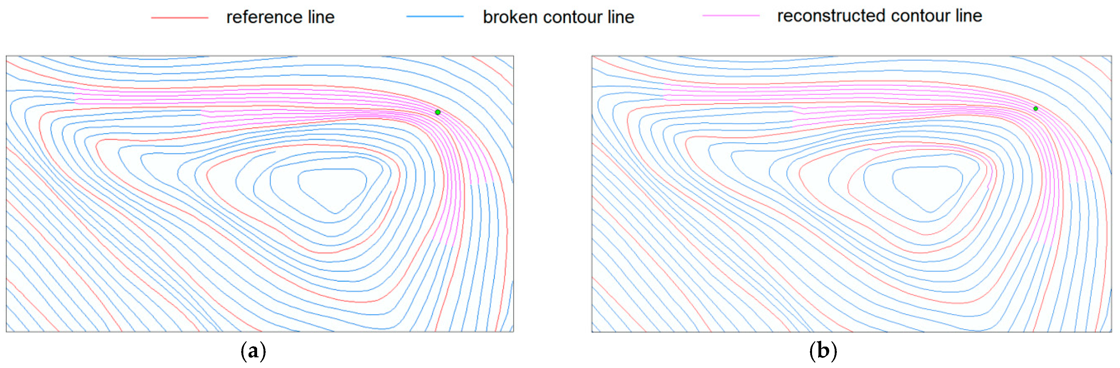
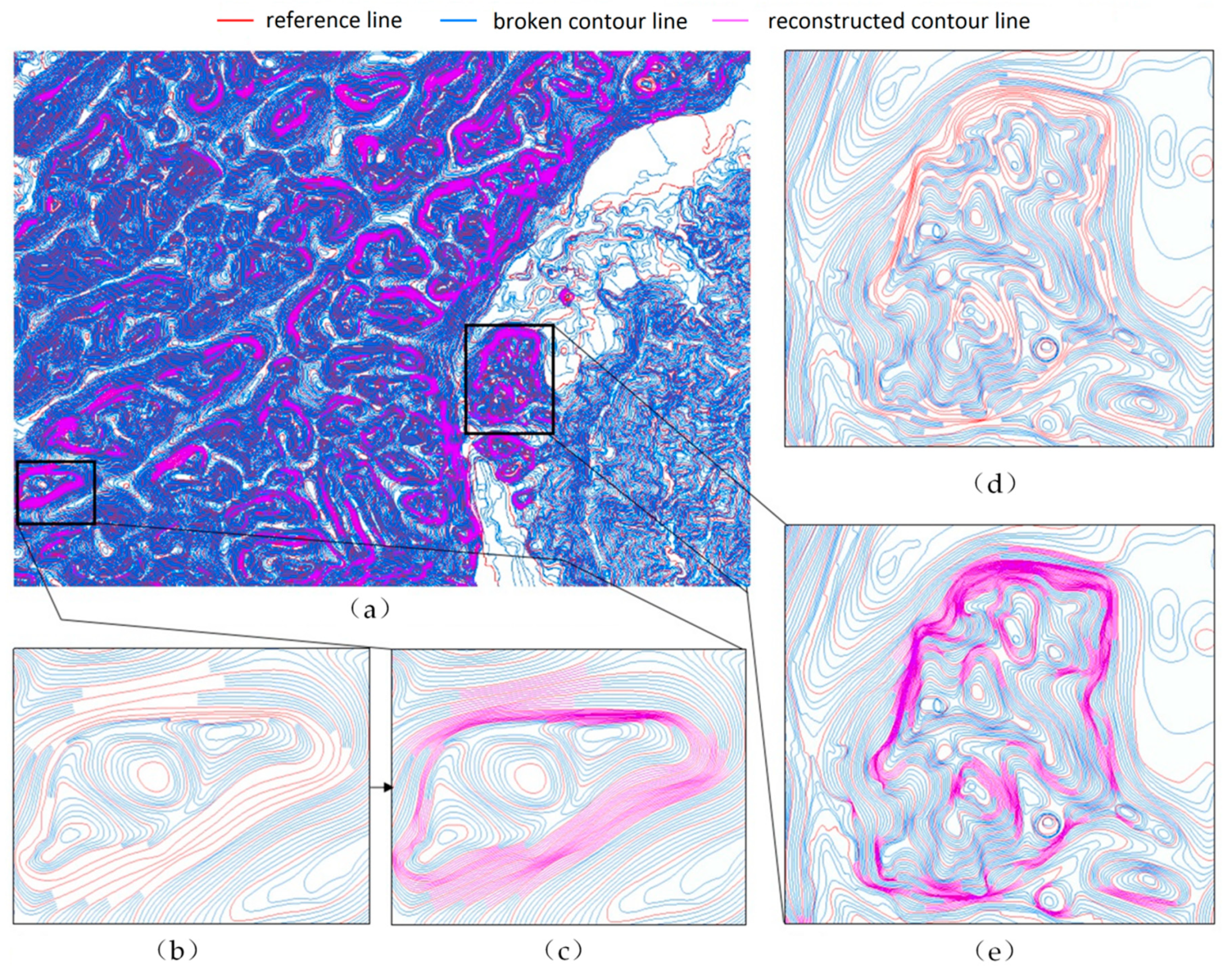
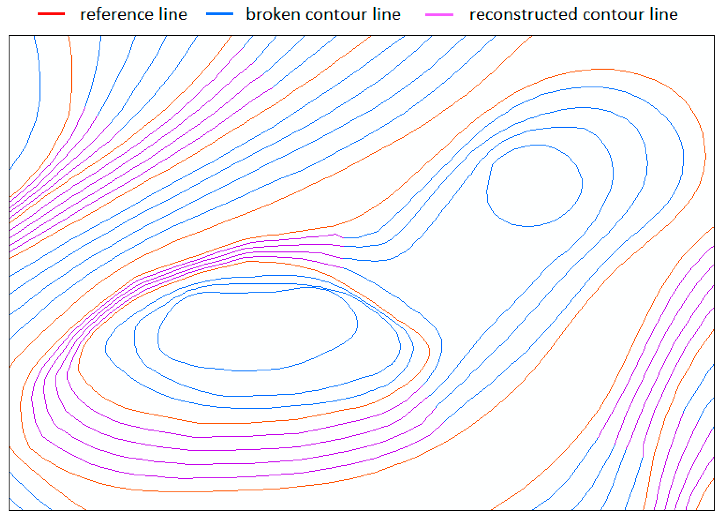
In terms of general analysis, the experimental results show that the proposed method is applicable for the reconstruction of both complex broken contours and general broken contours, with good universality.

(2)

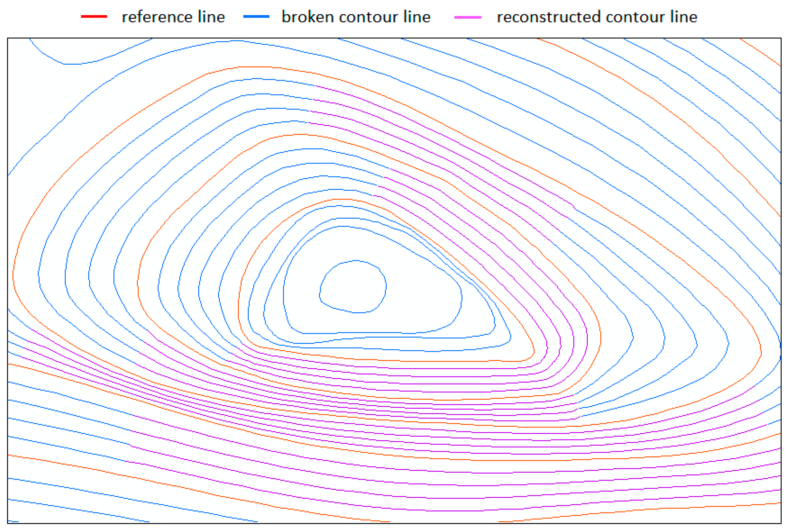
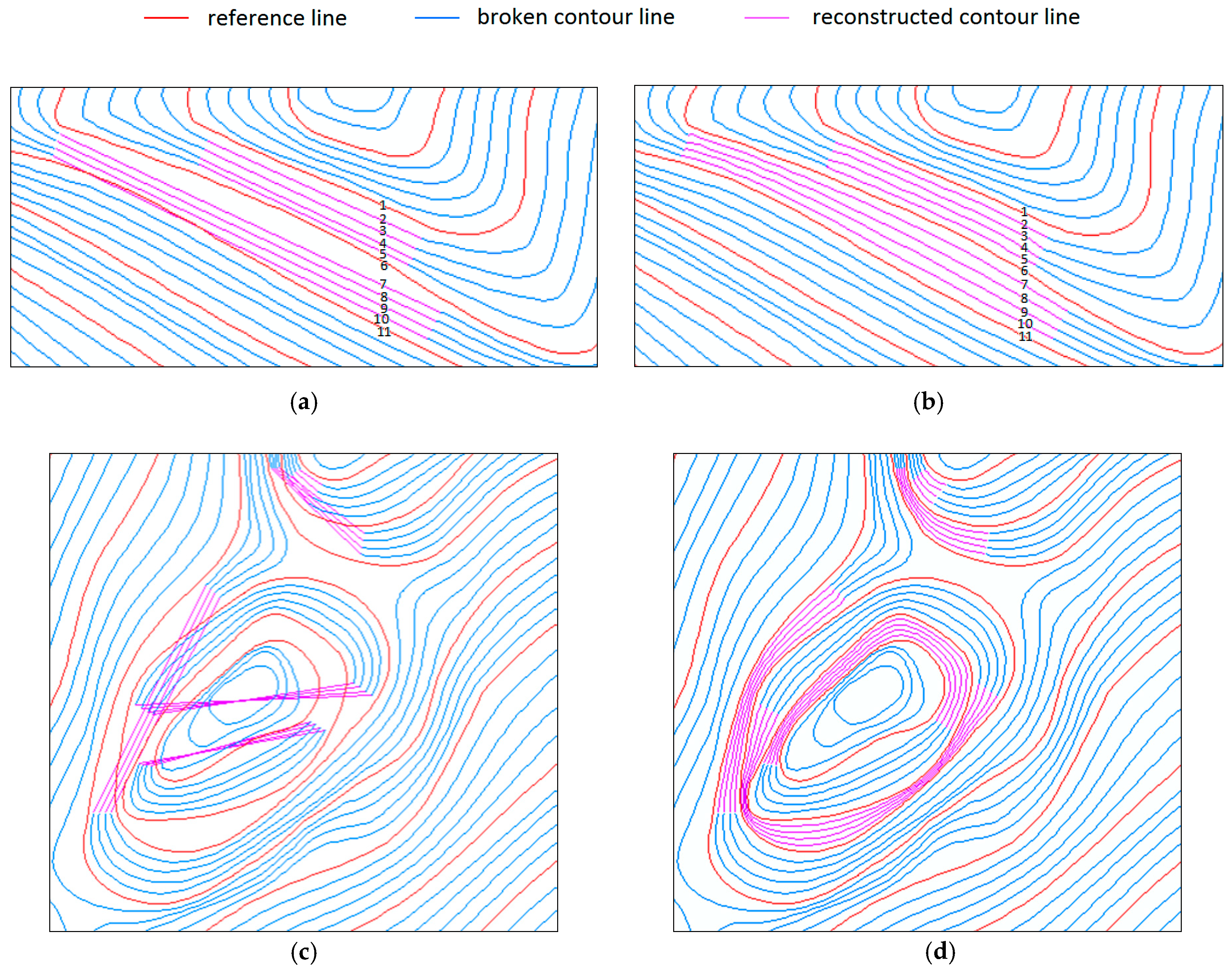
In terms of reconstruction accuracy, the reconstruction results were compared with results from the minimum point pair method under the same conditions. The method in this paper had better results for connection and reconstruction in a simple broken contour zone, and the reconstruction accuracy in a complex broken contour zone was significantly improved.

A leakage connection may occur by using our method when the similarity between the broken contour and the reference contour is low. In future research, more attention will be paid to the selection and optimization of reference contours to further improve the accuracy of the reconstruction of broken contour lines.

References

1. Samet, R.; Hancer, E. A new approach to the reconstruction of contour lines extracted from topographic maps. J. Vis. Commun. Image Represent. 2012, 23, 642–664. [Google Scholar] [CrossRef]
2. Spinello, S.; Guitton, P. Contour Line Recognition from Scanned Topographic Maps. Winter Sch. Comput. Graph. 2004, 12, 419–426. [Google Scholar]
3. Du, J.; Zhang, Y. Automatic extraction of contour lines from scanned topographic map. IEEE Int. Geosci. Remote. Sens. Symp. 2004, 5, 2886–2888. [Google Scholar]
4. Gul, S.; Khan, M.F. Automatic Extraction of Contour Lines from Topographic Maps. In Proceedings of the International Conference on Digital Image Computing: Techniques and Applications, Sydney, NSW, Australia, 1–3 December 2010; pp. 593–598. [Google Scholar]
5. Hancer, E.; Samet, R. Advanced contour reconnection in scanned topographic maps. In Proceedings of the International Conference on Application of Information and Communication Technologies, Baku, Azerbaijan, 12–14 October 2011; pp. 1–5. [Google Scholar]
6. Pouderoux, J.; Spinello, S. Global Contour Lines Reconstruction in Topographic Maps. In Proceedings of the International Conference on Document Analysis and Recognition. IEEE Comput. Soc. 2007, 2, 779–783. [Google Scholar]
7. Xin, D.; Zhou, X.; Zheng, H. Contour Line Extraction from Paper-based Topographic Maps. J. Infrom. Comput. Sci. 2006, 1, 275–283. [Google Scholar]
8. Ghircoias, T.; Brad, R. Contour Lines Extraction and Reconstruction from Topographic Maps. Ubiquitous Comput. Commun. J. 2011, 6, 681–691. [Google Scholar]
9. Arrighi, P.; Soille, P. From scanned topographic maps to digital elevation models. In Proceedings of the International Symposium on Imaging Applications in Geology, Liege, Belgium, 6–7 May 1999. [Google Scholar]
10. Min, F.U.; Xiao-Ning, L.I. Iteration approach for contour lines reconstruction based on breakpoint classification and orientation difference. J. Sichuan Univ. 2013, 50, 737–742. [Google Scholar]
11. Cheng, J.; Liu, P.; Wang, F. Comparison of Reconstruction Methods for Broken contour Lines on Raster Topographic Maps. Geomat. Sci. Eng. 2015, 35, 36–42. (In Chinese) [Google Scholar]
12. Xiaoya, A.N.; Liu, P.; Yun, Y.; Hou, S. A geometric similarity measurement method and applications to linear feature. Geomat. Inf. Sci. Wuhan Univ. 2015, 40, 1225–1229. (In Chinese) [Google Scholar]
13. Huttenlocher, D.P.; Klanderman, G.A.; Rucklidge, W.J. Comparing images using the Hausdorff distance. IEEE Trans. Pattern Anal. Mach. Intell. 1993, 15, 850–863. [Google Scholar] [CrossRef]
14. Fréchet, M.M. A few points on the functional design. Rendiconti del Circolo Matematico di Palermo (1884–1940) 1906, 22, 1–72. (In French) [Google Scholar] [CrossRef]
15. Alt, H.; Knauer, C.; Wenk, C. Matching Polygonal Curves with Respect to the Fréchet Distance. Comput. Geom. 2005, 30, 113–127. [Google Scholar]
16. Zhu, J.; Huang, Z.; Peng, X. Curve Similarity Judgment Based on the Discrete Fréchet Distance. J. Wuhan Univ. 2009, 55, 227–232. (In Chinese) [Google Scholar]
17. Schlesinger, M.I.; Vodolazskiy, E.V.; Yakovenko, V.M. Fréchet Similarity of Closed Polygonal Curves. Int. J. Comput. Geom. Appl. 2016, 26, 53–66. [Google Scholar] [CrossRef] [Green Version]
18. Eiter, T.; Mannila, H. Computing discrete Fréchet distance. See Also 1994, 64, 636–637. [Google Scholar]
19. Li, C.; Yin, Y.; Liu, X.; Wu, P. An Automated Processing Method for Agglomeration Areas. ISPRS Int. J. Geo-Inf. 2018, 7, 204. [Google Scholar] [CrossRef]
Figure 1. Schematic diagram of the minimum point pair method for reconstruction.
Ijgi 08 00008 g001
Figure 2. Schematic diagram of the breakpoint extension intersection identification matching method for reconstruction.
Ijgi 08 00008 g002
Figure 3. Connection mistakes: severely broken contour lines (area B) and the broken terrain of a contour line with a saddle shape (area C).
Ijgi 08 00008 g003
Figure 4. Diagram of the Fréchet distance between curves: (a) Fréchet distance between sparse nodes and (b) Fréchet distance between dense nodes.
Ijgi 08 00008 g004
Figure 5. Curve similarity calculation.
Ijgi 08 00008 g005
Figure 6. Diagram of broken contour line interpolation and connection.
Ijgi 08 00008 g006
Figure 7. Iteration processing results: (a) first-round reconstruction results (intercepted) and (b) one-iteration reconstruction result (intercepted).
Ijgi 08 00008 g007
Figure 8. The results and local amplification of the reconstructed broken contour lines in the experimental area: (a) overall results after reconstruction, (b) before reconstruction (severe cases of broken contour lines), (c) after reconstruction (severe cases of broken contour lines), (d) before reconstruction (complex terrain with broken contour lines), and (e) after reconstruction (complex terrain with broken contour lines).
Ijgi 08 00008 g008
Figure 9. The results and local amplification of the reconstructed broken contour lines in severe cases of broken contour lines.
Ijgi 08 00008 g009
Figure 10. The results and local amplification of the reconstructed broken contour lines in saddle-shaped terrain.
Ijgi 08 00008 g010
Figure 11. Comparison diagram of the reconstruction results between the minimum point pair method and the method in this paper: (a) the minimum point pair method (simple broken contour zone); (b) the method in this paper (simple broken contour zone); (c) the minimum point pair method (complex broken contour zone); (d) the method in this paper (complex broken contour zone).
Ijgi 08 00008 g011