Abstract
Based on probabilistic time-geography, the encounter between two moving objects is random. The quantitative analysis of the probability of encounter needs to consider the actual geographical environment. The existing encounter probability algorithm is based on homogeneous space, ignoring the wide range of obstacles and their impact on encounter events. Based on this, this paper introduces obstacle factors, proposes encounter events that are constrained by obstacles, and constructs a model of the probability of encounters of moving objects based on the influence of obstacles on visual perception with the line-of-sight view analysis principle. In realistic obstacle space, this method provides a quantitative basis for predicting the encountering possibility of two mobile objects and the largest possible encounter location. Finally, the validity of the model is verified by experimental results. The model uses part of the Wuhan digital elevation model (DEM) data to calculate the encounter probability of two moving objects on it, and analyzes the temporal and spatial distribution characteristics of these probabilities.
1. Introduction
Spatio-temporal analysis is generally applied to the visualization or prediction of spatio-temporal patterns of human or environmental phenomena. With the rapid increase in the amount of spatio-temporal data, spatio-temporal analysis has clearly attracted more and more attention [1]. There is more and more research on motion data, but the research on dynamic interaction in motion data is still in its infancy [2]. Meeting interaction is a spatio-temporal relationship (e.g., dynamic interactions between animals; rescues or meetings between people, etc.) that can be analyzed based on spatio-temporal trajectory data [3]. It is given that an individual’s movement trajectories can be interpreted as a discrete sequence of time-stamped known locations, which are also often referred to as anchor points or fixes. The spatio-temporal position between any two consecutive anchor points is uncertain, which results in the uncertainty of the encounter interaction based on spatio-temporal trajectory data. The degree of uncertainty of encounter increases with the presence of obstacles. For example, the mountain will block the rescuers’ sight and increase the difficulty of rescue. Even small groves and buildings will become obstacles for people to encounter, which affects the search operations, mainly reducing the success rate of search and rescue. In this sense, the study of the impact of the widely existing obstacles on the encounter of the moving objects can make the measuring method of the encounter uncertainty better, and improve the prediction level of the successful search and rescue; then, it will put forward an effective search algorithm to improve the efficiency of the search and rescue. In addition, the resulting encounter probability can answer the following questions. In many cases, one of the typical cases is that on a terrain barrier area S; a searcher is looking for a lost person, so how likely is the searcher to find the lost person? Where is the most likely place to encounter missing people?
In GIScience, time geography, as a basis for quantifying agents, especially analyzing mobile objects [4], represents a powerful framework for exploring how individual movements are affected by different spatio-temporal processes [5,6], and the resulting space-time prism can describe the temporal and spatial boundaries of object motion and divide the position in space and time into reachable or unreachable [6]. Space-time prisms and paths [7,8], as well as their extensions, provide the basis for the geographic analysis of geographically moving objects, such as quantifying time-space interactions between objects, etc. [9]. In movement ecology, the time-geography is an effective method for estimating the potential location area of an animal, such as its home range [10], using simulated space-time movement data testing [11], and can represent the randomness of the location of a moving object by the probability distribution over geospatial space [12,13,14].
If the potential location areas of two moving objects are likely to be adjacent or on the same location at a same time, then the meeting possibility of the two objects is also great. In this way, the intersection test of spatio-temporal potential location areas can be used to qualitatively judge the uncertainty of whether the two moving objects are likely to encounter in a time t. Winter and Yin [15] first proposed the calculation method of encounter probability, and described the meaning of encounter semantics, which is when two moving objects are located in the same discrete unit at the same time, they meet. This method has been used to calculate the dynamic interaction of wild animals [16], but it only applies to discrete space with determined units, and was not suitable for outdoor continuous space. Yin et al. [17] proposed an algorithm for the encounter probability of continuous space based on the following encounter semantics: the prerequisite for the two animals to meet each other is that their spatial distance does not exceed a given threshold (dmeet), such as visual distance.
Moving objects usually move in geospatial space, where the geographical environment in which moving objects occur is considered to be an important component [2]. Terrain barriers, roads, and road networks are spatial constraints that are relative to interactions, and should be considered in the interactive analysis of time geography. The distance-based encounter semantics ignores surface obstacles and their impact on encounter events. In general, the more obstacles there are, the less likely it is that two of the objects will meet. This means that the quantitative analysis of time geography needs to consider the actual obstacle space. For example, the literature [18,19] defines the extended space-time prism on the road network with obstacles and the rough space-time prism within the obstacle space, respectively.
This article will extend the distance-based encounter algorithm with two major improvements. First, it will introduce line-of-sight topographic visual analysis to study the encounter semantics in obstacle space. That is, two objects encounter each other if the distance between the two objects does not exceed dmeet and the lines of sight of the two moving objects are unobstructed. Here, we will develop a mathematical foundation to measure the semantics of the encounter. Second, in this paper, while studying the semantic formalization of obstacles in space, we fully consider the influence of the height of the moving object itself on the encounter probability, and give the different mobile object heights to create a map of encounter probability, which provides the basis for the excavation of the law of encounter and analysis of the maximum encounter probability.
2. Background
When it comes to the motion of multiple objects, it is meaningful to analyze the interaction between motion trajectories and visual analysis for various fields [20]. The encounter in obstacle spaces is an extension of the probability time geography based on line-of-sight analysis. The method of probability time geography and the theory of line of sight analysis are used to measure whether two moving objects meet in the obstacle space, and then assess the likelihood of encounter for analyzing the spatio-temporal behavior of the moving objects.
2.1. Encounter in Probabilistic Time Geography
Probability time geography is an extension of time geography based on probability [21]. Positional probability, as a key concept in probability time geography, is the probability of moving objects at a specific location at a time t [12], and provides the basis for the uncertainty measure of the encounter between individuals. Probability time geography has proposed a number of methods for calculating this position probability based on the motion state of the moving object. For example, the tracking data of vehicles [22], animals [23], and people [24] can be used in the calculation of location probabilities by statistical analysis and the spatio-temporal analysis method. These positional probabilities can form a two-dimensional probability density surface [25], which is also often referred to as utilization distribution in movement ecology, for modeling the heterogeneity of mobile objects in different accessible locations. A probability map is drawn by mapping these positional probabilities of a moving object to the map [26], and consequently can show the most likely position of the moving object at time t and the position where the moving object can be most likely be found.
The position probabilities provide the basis for calculating the likelihood of two moving objects meeting, and the resulting probability can answer the following questions [15]. What is the probability of encounter between two moving objects? Where are they most likely to meet? For any pair of moving objects A and B, the encounter probability in discrete space [15,26] can be expressed as:
where and are the probability of A and B distributed in a cell with an index of i. However, this algorithm is sensitive to cell definitions [17,26]. This means that different granularity in the same continuous space will bring different encounter probabilities. Yin et al. [15] introduced a perception distance threshold, and proposed a model of encounter probability based on this threshold. Irregular encounter areas are infinitely subdivided into regular grids, and then calculated by integrals. However, this algorithm does not take into account the effect of obstacles on visual perception.
2.2. Line-of-Sight Topographic Visual Analysis
As a method for deriving areas of visibility from any given vantage point or area, viewshed analysis is an important tool that is used to describe the visible spatial structure of an environment, and hence can answer questions such as the following. In movement ecology, can animals and natural enemies see each other in the wild? Is there a significant interaction between the two species? [27]. In the field of GIS, viewshed analysis has been proven to be the most popular methodology and an important function for quantifying visibility [27,28,29], and its application is now commonly practiced in a range of fields, including road planning [30] and terrain exploration [31,32]. We will use the viewshed analysis tool to build the encounter model.
The line-of-sight (LoS) topographic visual analysis refers to the technical method to judge whether any two points on the terrain are visible. It establishes the LoS between the viewpoint and the target point, and determines whether it is visible by judging whether there are obstacles that obstruct the vision [29] (Figure 1). The most important advantage of this method is that terrain visibility is only determined by a simple geometric relations of points. However, traditional visibility analysis methods [33] failed to consider the effect of the height of the observer on the visibility, and thus the viewshed is a poor measure of visibility from a human perspective, e.g., encounters between people.
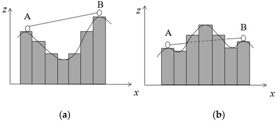
Figure 1.
Topographic line-of-sight analysis: (a) visible; (b) invisible.
Nutsford et al. [27] proposed a visual analysis method that takes into account the observer’s height in the following two factors: the distance between a perceived object and the observer, and the vertical dimension (i.e., slope and aspect) of the terrain. However, this method fails to take into account the individual’s ability to perceive the environment, such as the distance of vision. Obviously, in the scene of the encounter, the two individuals not only need to meet the conditions of the vision (to ensure that there is no obstacle between the individuals), but also need to meet the perceptible conditions.
3. The Encounter Probability Model Based on Obstacle Space
The encounter is first of all a discovery, followed by further contact (such as predation) or evasion (such as escaping natural enemies). The encounters that we study are the most likely discoveries to provide decision support for individuals planning behavior early (such as contact or evasion).
3.1. The Semantics of Encounter in Obstacle Space
The encounter semantics in the obstacle space can be regarded as an extension of the encounter semantics in a continuous space (Table 1). The encounter semantics in a continuous space are defined as the distance between two individuals ≤ dmeet; within this threshold, an individual can perceive (e.g., visual, auditory, olfactory, sensory, etc.) to another individual, or vice versa [17]. The encounter semantics of continuous space is different from that of discrete space (two individuals are in the same discrete unit at the same time), but both ignore the obstacles inside the space. The obstacle space can be simply viewed as a composite of continuous space and obstacles. This means that the encounter semantics of the obstacle space, while inheriting that of the continuous space, needs to consider that there are no obstacles between the two individuals that can hinder the individual’s perception. For example, from a visual point of view, there should be no obstruction (e.g., buildings, mountain head) to the line of sight between two individuals that can meet.

Table 1.
Evolution of encounter semantics.
From the above analysis, we can see that the encounter semantics in the obstacle space include two necessary conditions—distance threshold and barrier-free features—which can then be used to determine if an encounter between two individuals is likely to occur.
- (1)
- Distance includes path distance and Euclidean straight line distance. The setting of the distance threshold is closely related to the type and characteristics of the individual. In movement ecology, the distance threshold for potential encounters varies with species. For example, the distance thresholds for deer and lion populations are 50 m [34] and 200 m [35], respectively.
- (2)
- Barrier-free features are relative to the location of the two individuals. Under normal circumstances, the obstacle characteristics of spatial features are related to the type of sensory perception. For example, a two meter-high fence is an obstacle for the visual sense, but not necessarily for the hearing sense. In GIScience, sight-line visual analysis can dynamically detect the visibility between two points, so it can also detect whether there is an obstacle blocking two viewpoints. The traditional visibility analysis mainly considers the terrain environment, while ignoring the individual factors such as the individual’s height and the individual’s perception characteristics. This also reminds us that the visual analysis for potential encounter measures needs to take into account individual factors.
3.2. Encounter Events in Obstacle Space
The encounter semantics provides a theoretical basis for the definition of encounter events. From the perspective of probability theory, the encounter event is a random event, which is a phenomenona in which two independently moving individuals randomly meet.
3.2.1. Condition of Encounter Events
The encounter semantics provides the necessary conditions for the occurrence of encounter events, namely the distance conditions and barrier-free conditions. Since the necessary conditions are not sufficient conditions, even if the necessary conditions are satisfied, the two individuals cannot always meet each other. This raises the question of how to judge whether the encounter event can occur in time geography, that is, the judgment condition of the encounter event.
Time geography provides some ideas and methods for solving the above problems. Such methods as time geography often use the maximum value to describe the uncertainty of the variables. For example, the maximum possible speed represents the uncertainty of the individual’s speed; the largest possible range (or prism) represents the individual’s space-time reachable domain (or uncertainty of space-time location) to maximize the capture of all of the possible positions of an individual. Similarly, we have no more knowledge to deny that the necessary conditions are not sufficient conditions. Taking these necessary conditions as sufficient conditions is a maximization of meeting conditions, which is in order to maximize the capture of encounter events. Thus, when the necessary conditions (distance conditions and barrier-free conditions) are satisfied at the same time, the encounter event can be considered to have occurred. On the contrary, if there is a condition that is not met, the encounter event must not occur. Therefore, the necessary conditions can be used to determine the distinguishable zero-dimensional relationship, meet, and ascertain whether its qualitative likelihoods are impossible or possible.
Obviously, the test of the meeting conditions (distance conditions and barrier-free conditions) completely depends on the location of the two individuals and the surrounding geographical environment. Based on the individual’s location and geographical environment data, we can calculate the distance between two individuals and analyze whether there are obstacles between them, and therefore can determine whether the encounter events of the two individuals are likely to occur.
3.2.2. Building the Event that Individuals Were at Specific Locations at a Specific Time
In time geography, each location where an agent is located can usually be abstracted into a geometric point [9]. Thus, the position of the individual A can be regarded as a point, and can be labeled as LA = {lA|lA [1], lA[2], …}. In three-dimensional (3D) space, each position lA is a value of the variable LA. Similarly, the position of individual B can be labeled as LB = {lB|lB[1], lB[2], …}. Under the given geographical environment and time t, the encounter events of two individuals A and B respectively located at specific positions lA and lB can be described as follows:
where:
Emeet represents the encounter event.
HA (resp. HB) is the height of individual A (resp. B).
||| - ||| represents a distance operator between two spatial locations (such as the viewpoint of two individuals) in three-dimensional space.
dmeet is the threshold that characterizes the maximum distance across which two individuals can meet, such as the maximum distance of the line of sight.
f(x, y) is the elevation function of the surface, expressing the elevation value at the two-dimensional position (x, y), such as zA = f (xA, yA), zB = f (xB, yB).
is the line between two points: lA’(xA, yA, zA + HA) and lB’(xB, yB, zB + HB), where lA’(xA, yA, zA + HA) is a point in three-dimensional space, and its height is higher than point lA (xA, yA, zA) by HA (Figure 2).
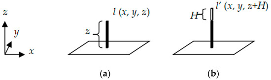
Figure 2.
Terrain elevation (a) and viewpoint height (b).
means that there is no intersection between the line and the surface , or there is no obstacle between the two points lA’ and lB’. The encounter event is shown in Figure 3.
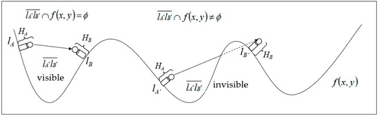
Figure 3.
Two relationships between sight and terrain.
It can be seen from the above that an encounter event can occur when two encounter conditions ( and ) are satisfied. Obviously, the occurrence of the event means that at time t, the individual A must be located at the position lA (denoted as event ), and B must be located at lB (denoted as ). Therefore, the event can also be described as:
where the events and are independent, which is due to the assumption that the movements of A and B are independent of each other. In addition, since an individual can only be located in one of a number of locations in a potential location area [26], the event of the individual A located at lA[1] and the event at lA[2] are mutually exclusive. Further, a pair of individuals, A and B, can only be located in one of a plurality of position pairs (e.g., (lA[1], lB[1]), (lA[1], lB[2]), …) at the same time, and thus the event in position pairs (lA[1], lB[1]) and in (lA[1], lB[2]) are mutually exclusive.
3.2.3. Building the Event that Individuals Were Together at a Specific Time
The sample space of event is the potential location area of individual A at time t, which can be denoted as . This can be written as: = = {lA[1], lA[2], …}. Similarly, the sample space of event can be denoted as = = {lB[1], lB[2], …}. Once two sample spaces and are owned, the event of two individuals A and B meeting at time t can be calculated as follows:
where the sample space of the event, which is a composite of events and , can be obtained by a Cartesian product operation as: . Equation (4) is a six-dimensional (6D) space, i.e., the Cartesian product of two three-dimensional variables of lA and lB: lA(x, y, z) × lB(x, y, z). The time t is a constant rather than a variable, so it is not seen as one dimension. Although lA and lB are variables in three-dimensional space, the lA and lB are units in the surface based on discrete structure, and the label of each cell is a tuple, such as lA[1] and lA[2], instead of two tuples (row, column). In this way, lA and lB can be identified by a one-dimensional array, and thus can be traversed by an operation symbol of union.
Since is a 6D space, its presentation in a 3D space requires a dimensionality reduction method. Suppose that the heights of the two individuals A and B are both one meter, their reachable domains and are the same, and can be described by the following DEM matrix:
In this way, we can transform the 3-D space into 0-D 9 units (center points), in order to convert a 6-D space into nine 3-D subspaces: , , , (Figure 4). Each subspace can be expressed in three dimensions and can be used to visually analyze whether an encounter event between two individuals is possible. For example, in sample space , A can see B on , , , , , and , while others are not visible.
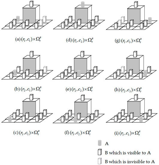
Figure 4.
Discretized representation of a four-dimensional sample space.
3.2.4. Building the Event that an Individual at a Specific Location Encountered Another
It is also possible to build the event that an individual A at a specific location lA met another individual B at time t, which is denoted as . In this event, the position of individual A is fixed, while that of B is variable and uncertain, which is one or more locations in the reachable area of B. In Figure 4a, the individual A (cylinder) at a position point is likely to encounter B (solid cylinder) at 7 positions, and it is impossible to meet the B (dashed cylinder) at 2 positions due to the obstacles. This event can be built for each location as:
Based on this, we can build the event that the individual A at the location lA met B, which is denoted as at least once during the tracking duration. This event can be built for each location as:
where the encounter event is modeled using Equation (5). However, it is a non-mutually exclusive, since objects can interact at multiple times [26].
3.2.5. Building the Event that Individuals Encountered during the Tracking Duration
Events that two individuals met at any time t at any location pair (lA, lB) denoted simply as , can also be derived from Equation (4), which model the event that the individuals met at each time step.
where the events at different points in time, such as and , are not mutually exclusive, that is, encounter events can occur multiple times at different points in time.
3.3. Encounter Probability in Obstacle Space
3.3.1. Calculating the Probability that Individuals were at Specific Locations at a Specific Time
According to Equation (2), the uncertainty of the encounter event can be converted into that of two simultaneous events and . This means that lA and lB can be considered as two random variables of this encounter event. For a pair of individuals A and B moving independently of each other, the probability of the can be denoted as , and can be calculated according to the multiplication formula of independent events in probability theory. This can be written as:
where records the probability for individual A at position lA at time t, and records the probability for B at position lB at time t. The can be calculated for all of the positions in a map at any time, and is a joint probability of and . The flowchart for a step-by-step probability calculation is shown in Figure 5.
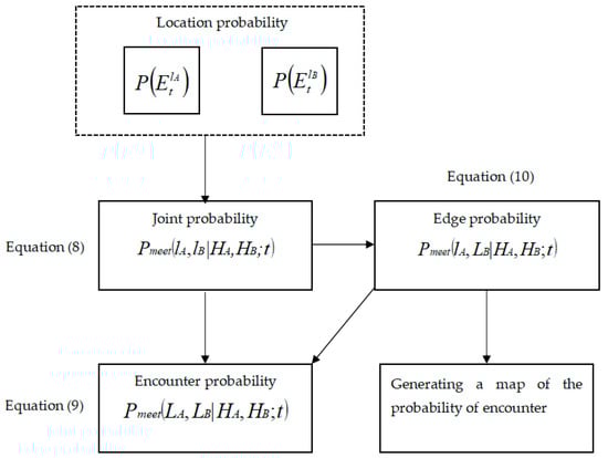
Figure 5.
The probability calculations.
3.3.2. Calculating the Probability that Individuals Were Together at a Specific Time
Since the encounter events at different location pairs for two individuals are mutually exclusive (i.e., two individuals can only be located in one location pair at a point in time), the probability that two individuals interacted at specific time t at any location pair (LA and LB) can be calculated simply by summing the interaction probabilities for all of the location pairs within the , and can be expressed as:
where the probability formula can be regarded as the integral of Equation (8) in area ; both lA and lB are three-dimensional spatial points, so the corresponding integral is triple. A discrete type of Equation (9) is derived in Section 4.3. As discussed earlier, the method proposed in this paper is based on the assumption that individual motions are independent of each other. In fact, the occurrence of encounter events has an impact on the independence of individual actual movements, but does not affect the assumption that the null hypothesis (i.e., individual motion is independent of each other) is correct, because the null hypothesis itself is the hypothesis to be tested [17]. This calculation of Equation (9) can then be repeated for each time slice t to determine how interaction probabilities fluctuate over time [26], as well as to assess the independence between individual movements and the influence of encounter events on the independence of subsequent movements.
3.3.3. Calculating the Probability that an Individual at a Specific Location Met Another
According to Equation (5), the probability of the event , which is denoted as , is an edge probability of Equation (8), where A is in a known location, and B is in all of the possible locations nearby at the same time. It can be calculated by the addition rule of the mutually exclusive event as follows:
Based on the above probability and Equation (6), it is also possible to calculate the probability of the event , which is denoted as . This probability can be written and calculated as:
Since events at different times are not mutually exclusive, this probability requires the additional formula of general events in probability theory. Furthermore, mapping the probability of the location of each lA in the reachable domain creates a probability map of individual A encountering B [26]. Such a map illustrates the most likely places that A can meet B over the specified time interval.
3.3.4. Calculating the Probability that Individuals Encountered During the Tracking Duration
According to Equation (7), the probability that two individuals encountered at any time t at any location pair (lA, lB) can be denoted as , and can be calculated by the probability addition formula of non-mutually exclusive events. This can be written as:
where is a single number that represents the probability that A and B encountered at least once during the entire tracking interval.
4. Application
4.1. DEM Modeling of Continuous Space
Geospatial space can be considered continuous, and can be expressed using the GIS field model; based on this model, we have previously constructed the encounter probability formula. However, both the judgment of the encounter event and the calculation of the integral function in the encounter probability formula require a discrete spatial data model, such as the discrete space-time aquarium [15] and the voxel-based probabilistic space-time prisms [16]. Judgment of encounter events requires an analysis of distances and visibility conditions between location points. Integral operations need to analyze the probability of location points. These location points are infinite in contiguous space, and computers cannot normally analyze an infinite number of points one by one. Therefore, the calculation of the probability of encounter in a continuous obstacle space requires the use of a discrete spatial data model.
As a discrete model for expressing terrain, DEM has become the basic spatial data model for visibility analysis in the GIS field, and thus can be used for the calculation of encounter probability. In DEM, a cell is a square or rectangle with a certain height value; the coordinates and elevation of each cell are expressed by those of the center point of the unit, respectively. Once we have the DEM data and the location and height information of the two individuals, we can determine whether they are likely to meet. For illustration, the encounter probability in the obstacle space was applied to the DEM data with a resolution of 30 m × 30 m in Wuhan, China (http://www.gscloud.cn/) (Figure 6).
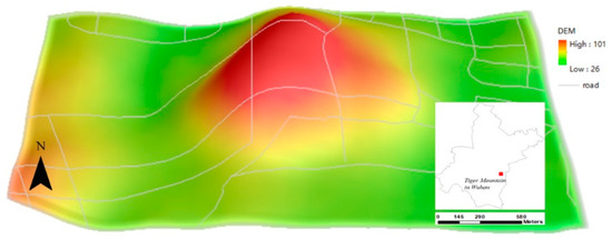
Figure 6.
DEM.
4.2. Calculation of Positional Probability
The motion of two objects is assumed to be independent of each other, and moving objects usually have a certain directional preference for the destination. Some scenarios that are consistent with the hypothesis of this experiment can be like this, such as human movement, including the potential movements of missing persons and recreationalists [36]. Classical time geography [21] can calculate the reachable domain of an individual at a given moment in time based on the spatio-temporal information of the starting and ending points and the maximum speed of the individual. Such reachable domains are collections of discrete units in DEM. Given the reachable domains of two individuals A and B in the DEM at time t: = {lA[1], lA[2], …}, and = {lB[1], lB[2], …}, where lα indicates the center point of the unit where the individual α is located, and represents the set of potential units (labeled as lα) of individual α at time t (Figure 7). and contain 365 and 360 cells, respectively.
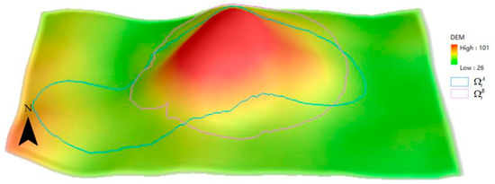
Figure 7.
The reachable ranges and of the two individuals A and B.
Probabilistic time geography [13,14] provides a means of assigning probabilities to an individual’s potential locations. The probability distribution of an individual α in the potential location area can also be derived by an inverse distance-weighting function using the following equation, as per Downs et al. [16]:
where is the probability that the individual α is located in the cell lα[k] at time t, sα is typically the expected location of individual α at t, and is the reciprocal of the distance between two points sα and lα[k] in 3D space.
4.3. Calculation Method of Encounter Probability
Due to the additive nature of integrals, i.e., an integral over a surface equals the sum of integrals over disjoint units that cover the surface, we can treat each of the unit regions in space-time separately, and add them together once the computation is done [37]. It is possible to convert the encounter probability formula from continuous-type to discrete-type, thus realizing the conversion of the probability formula of the encounter from the mathematical model to the model that can be calculated in the computer. This conversion mainly includes two aspects: converting the point of continuous space and the probability on it into a discrete unit and the probability on it; converting the integral operation into a sum operation. Equation (8) is the probability of encounter of two individuals at a given pair of points, which can be the center point of the unit in discrete space, so that this formula can be directly applied to discrete spaces.
Equation (9) is the probability of encounter of two individuals at time t, and its discrete-type can be written as:
where the probability provides the basis for Equation (12) to calculate the probability of encounter in discrete space and over time. Since lA and lB are represented by a one-dimensional tuple, the two summation operators can traverse the one-dimensional array of lA and lB, respectively. Obviously, Equation (14) is also the summation form of joint probability.
In addition, Equation (10) is the probability that an individual at a given position can meet another individual at time t, and its discrete-type can be written as:
where the probability provides the basis for the calculation of Equation (11) in discrete space. Moreover, in order to calculate the probability of encounter, we also need to set these parameters: ① the movement of two individuals A and B is independent, ② the heights HA and HB are one meter and two meters, and ③ dmeet = 80 m.
5. Results
In order to show the probability of encounter on the plane in the results, the grayscale map better reflects the range of the reachable domain. The projections of the given reachable areas and in (x, y) space are shown in Figure 8. Let the center point of area represent the expected location sα of individual α at t. According to Equation (13), we can calculate the probabilities of each individual in its own reachable units, and get the probability distribution maps of two individuals A and B at time t, as shown in Figure 9. As can be seen from the figure, the probability value in the center of the reachable area is the largest, and the farther away the individuals are from the center, the smaller the probability. In addition, different reachable areas of individuals lead to different probability distributions in their respective reachable domains.
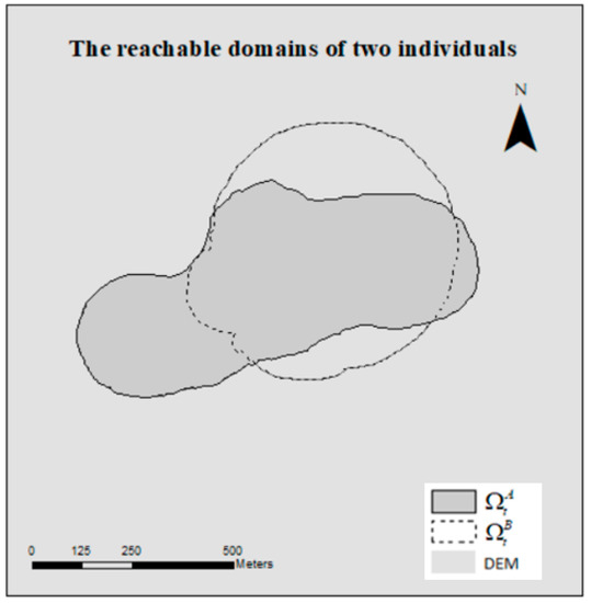
Figure 8.
The reachable domains of two individuals at time t.
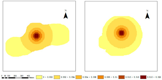
Figure 9.
Probabilities distribution of individuals A and B.
In the obstacle space, taking individual A as a seeker as an example, at the specific time t, for any potential position pair (lA, lB), if the distance between them is less than dmeet and there is the terrain obstacle factor, the encounter probability can be calculated according to Equation (8). Furthermore, according to Equation (15), we can also calculate the probability of individual A located at given point lA in encountering individual B in , and use this probability as the attribute of the point lA. Then, the sum of the attributes of each location lA in , which is the probability of individual A can encounter B at time t, is calculated as 0.036, which is the result of Equation (14). Since individuals A and B are symmetrical in Equation (14), when the seeker is individual B, the encounter probability of individual B meeting individual A is also 0.036.
The probabilistic attributes of each location point lA in are mapped to the DEM, resulting in a probability map of A encountering B in the obstacle space (Figure 10a). Similarly, we can also get a probability map of B encountering A (Figure 10b). The green base map is the DEM data with the road line and the potential location areas of the individuals A and B. The darker the color, the higher the value. As can be seen from the figure, the encounter probabilities of moving objects A and B are respectively larger in the center of each reachable range and . This result is related to the method of generating the positional probability of an individual by the inverse distance weighting method; however, it does not affect the validity of the model presented. It is worth mentioning that differences in the visual distance (the farthest distance can be seen), reachable domain, and probability distribution between individuals results in the differences in the encounter probability maps to a certain extent; that is, the probability map of A meeting B is different from that of B meeting A [17].
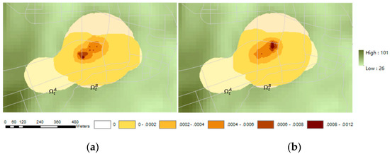
Figure 10.
Probability map of A meeting B (a) and that of B meeting A (b) in obstacle space.
In order to compare the influence of obstacles on the encounter, here we calculated the encounter probability between individuals A and B without considering the obstacle factor according to Equations (14) and (15). In the case of ignoring obstacles, Equation (14) calculates the probability of encounter as 0.055, which is significantly larger than the encounter probability of 0.036 in obstacle scenarios; Equation (15) can be used to generate the probability map of A meeting B (Figure 11a) and that of B meeting A (Figure 11b). Compared with Figure 10 and Figure 11, there is a significant distinction in probability distribution and density, which fully reflects the influence of obstacles on the encounter event.
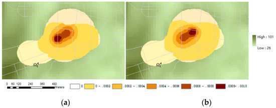
Figure 11.
Probability map of A meeting B (a) and that of B meeting A (b) without considering the obstacle factor.
The experimental results demonstrate the effectiveness of the model, which improves the measure of encounter probability in the real environment, as well as the prediction level of the location of the maximum probability of encounter.
6. Discussion
From the point of view of the present time geography, this paper expands extends the interaction probability from homogeneous space to obstacle space by considering the influence of obstacles on spatial interaction. In this study, we implemented these algorithms in Python with some DEM data from Wuhan, and verified the effectiveness of the proposed algorithm model using ArcGIS. The experiments show that the probability of encounter is different between barrier-free space and obstacle space, as well as subject to individual height, surface elevation, and individual visual ability. When using the DEM data to calculate the encounter probability, the following points need to be noted, such as for example, parameter settings, obstacle handling, and probability map generation. Combined with the model in this article, the content can be expanded and analyzed from the following aspects.
First, with respect to the setting of the distance threshold dmeet, it has a greater influence on the measurement result of the encounter interaction, because the larger threshold value will generate a larger encounter probability, and is determined primarily by the characteristics of the individuals and the environment. For example, in the lion’s interaction analysis, the interaction threshold is set to 200 m, because lions from the same group are often observed within this distance [35]. In the interaction analysis of deer, the threshold based on visual observation was set to 50 etersm [6]. In this paper, an appropriate dmeet = 80 m is chosen to be based solely on the grid cell with a side length of 30 m, which is consistent with the purpose of this paper, that is, to validate the effectiveness of the interaction probability model in obstacle space for mobile objects of different types and characteristics. Depending on the specific research objective, the spatial threshold can be adjusted up or down until the measurement results are less sensitive to this parameter [17].
Second, when line-of-sight topographic visual analysis is used, the problem of the effect of terrain on encountering is transformed into the problem of the intersection of the line of sight between two moving objects and the surface. Line of sight indicates the line between LA’ (xA, yA, zA + HA) and LB’ (xB, yB, zB + HB). That is, considering the height of the moving objects A and B itself, the impact on the encounter problem is more in line with the actual application scene. In most cases, the line of sight does not pass through the central point of the unit through which it passes, but in experiments, the only elevation of the unit is compared with the line of sight. In a sense, the improvement of the algorithm can be achieved by reducing the size of the grid, or by substituting the elevation surface function for elevation grid structure.
Third, when generating a map of encounter probability between moving objects, a moving object needs to be designated as a seeker. Although the probability function of two individuals’ encounter is independent of the order of individuals, the map of the probability of encounter is related to specific individuals. That is to say, in the same encounter phenomenon, the maps of the encounter probability of different individuals are different.
Finally, in the experiment, the reachable domains of the two individuals were specified. Time geography provides a framework for calculating reachable domains based on the individual movement trajectory data. Since the main purpose of this paper is to verify the mechanism of the influence of obstacles on the probability of encounter, there is no step to calculate the potential location area in the experiment, which makes the method validation have certain limitations. One possible area of future work is to integrate the actual reachable domain in the interaction analysis according to the spatiotemporal trajectory data and the maximum travel speeds of moving objects subject to individual abilities, terrain (slope, aspect), land cover, and the presence of barriers [36,37]. Additionally, as for the calculation of location probability, we only consider the distance factor in the inverse distance weight function. Another future work is to consider the influence of environmental constraints (including obstacles) on location probability.
7. Conclusions
This research introduces a method of calculating the encounter probability of two moving objects in the terrain obstacles space, which improves the traditional algorithm of the encounter probability in the plane space. It mainly considers the influence of terrain factors and the height of the moving object itself on the encounter issue, and further transforms the influence into the intersection of the line-of-sight between the two moving objects and the ground surface. This paper considers continuous space and time, and provides an analytical framework for quantitatively measuring the likelihood of two individuals encountering in an obstacle space. For simulation, considering the discrete nature of the computer environment, the paper converts the original formulas into a discrete case (see Equations (14) and (15)). So far, time-geography has relatively perfect methods for measuring random encounters.
Several extensions and improvements to our model should be discussed in future work. Since the time-geography encounter probability algorithm has reached an acceptable realism to analyze common tracking data in an obstacle-constrained environment, we plan to validate our approach through a wide range of datasets and real-world geography. Realistic geospatial space is not just a space with terrain factors as obstacles. In many environments, indoors or outdoors, it may be abstracted as an insurmountable obstacle space, such as buildings and fences. An attractive extension of the geographical environment’s impact on encounter events can be to consider time-varying constraints rather than permanent obstacles. This will allow for the handling of temporary items, such as those with temporary events (such as stages, tents), which complicate the study of encounters between spatio-temporal data. Also, we may consider some barriers that can be passed internally, and these barriers apply to different constraints. For example, lawns and shrubs in parks can be considered as permeable barriers, and for pedestrians, the maximum speed of such obstacles is abnormal [19]. Therefore, the follow-up work is the promotion of the model in the reality of other heterogeneous obstacles and network space, which introduce different forms of obstacles, and improve the traditional Euclidean distance to the road network distance and more solutions.
A final note, future work could use Monte Carlo (MC) simulation to account for two cases after meeting for the first time (1) getting away from each other; and (2) moving toward each other. These would be more useful to modeling the two corresponding cases (1) animal movements and (2) human movements (e.g., rescuing people, as mentioned in the article).
Author Contributions
Conceptualization, Z.-C.Y. and H.L.; methodology, Z.-C.Y. and H.L.; validation, H.L.; formal analysis, Z.-C.Y. and H.L. and Z.-H.-N.J.; investigation, S.-J.L.; resources, J.-Q.X.; data curation, H.L.; writing—original draft preparation, H.L.; writing—review and editing, Z.-C.Y., H.L. and Z.-J.Z.; supervision, Z.-C.Y.; project administration, Z.-C.Y.; funding acquisition, Z.-C.Y.
Funding
Zhang-Cai Yin has been supported by grants of the National Key R&D Program of China Grant Number: [2017YFB0503700].
Acknowledgments
Thanks are due to Zhang-Cai Yin for valuable advice and inspiration. The completion of this article is also inseparable from the technical support of my classmates.
Conflicts of Interest
The author declares no conflict of interest.
References
- An, L.; Tsou, M.H.; Spitzberg, B.H.; Gupta, D.K.; Gawron, J.M. Latent trajectory models for space-time analysis: An application in deciphering spatial panel data. Geogr. Anal. 2016, 48, 314–336. [Google Scholar] [CrossRef]
- Zhang, P.; Beernaerts, J. A Hybrid Approach Combining the Multi-Temporal Scale Spatio-Temporal Network with the Continuous Triangular Model for Exploring Dynamic Interactions in Movement Data: A Case Study of Football. Int. J. Geo-Inf. 2018, 7, 31. [Google Scholar] [CrossRef]
- Long, J.A.; Webb, S.L.; Nelson, T.A.; Gee, K.L. Mapping areas of spatial-temporal overlap from wildlife tracking data. Mov. Ecol. 2015, 3, 38. [Google Scholar] [CrossRef] [PubMed]
- Kuijpers, B.; Othman, W. Modeling uncertainty of moving objects on road networks via space–time prisms. Int. J. Geogr. Inf. Sci. 2009, 23, 1095–1117. [Google Scholar] [CrossRef]
- Long Jed, A. Quantifying spatial-temporal interactions from wildlife tracking data: Issues of space, time, and statistical significance. Procedia Environ. Sci. 2015, 26, 3–10. [Google Scholar] [CrossRef]
- Long, J.A. Toward a kinetic-based probabilistic time geography. Int. J. Geogr. Inf. Sci. 2014, 28, 855–874. [Google Scholar] [CrossRef]
- Miller, H.J. A measurement theory for time geography. Geogr. Anal. 2015, 37, 17–45. [Google Scholar] [CrossRef]
- Miller, H.J.; Bridwell, S. A field-based theory for time geography. Ann. Assoc. Am. Geogr. 2009, 99, 49–75. [Google Scholar] [CrossRef]
- Downs, J.A. Time-geographic density estimation for moving point objects. In Geographic Information Science. GIScience 2010. Lecture Notes in Computer Science; Fabrikant, S.I., Reichenbacher, T., van Kreveld, M., Schlieder, C., Eds.; Springer: Berlin/Heidelberg, Germany, 2010; Volume 6292, pp. 16–26. [Google Scholar] [CrossRef]
- Katajisto, J.; Moilanen, A. Kernel-based home range method for data with irregular sampling intervals. Ecol. Model. 2006, 194, 405–413. [Google Scholar] [CrossRef]
- Downs, J.; Horner, M.; Lamb, D. Testing time-geographic density estimation for home range analysis using an agent-based model of animal movement. Int. J. Geogr. Inf. Sci. 2018, 32, 1505–1522. [Google Scholar] [CrossRef]
- Winter, S. Towards a probabilistic time geography. In ACM SIGSPATIAL GIS 2009; Mokbel, M., Scheuermann, P., Aref, W.G., Eds.; ACM Press: New York, NY, USA, 2009. [Google Scholar] [CrossRef]
- Winter, S.; Yin, Z.C. Directed movements in probabilistic time geography. Int. J. Geogr. Inf. Sci. 2010, 24, 1349–1365. [Google Scholar] [CrossRef]
- Song, Y.; Miller, H.J. Simulating visit probability distributions within planar space-time prisms. Int. J. Geogr. Inf. Sci. 2014, 28, 104–125. [Google Scholar] [CrossRef]
- Winter, S.; Yin, Z.C. The elements of probabilistic time geography. GeoInformatica 2011, 15, 417–434. [Google Scholar] [CrossRef]
- Downs, J.A.; Horner, M.W.; Hyzer, G.; Lamb, D.; Loraamm, R. Voxel-based probabilistic space-time prisms for analysing animal movements and habitat use. Int. J. Geogr. Inf. Sci. 2014, 28, 875–890. [Google Scholar] [CrossRef]
- Yin, Z.C.; Wu, Y.; Winter, S.; Hu, L.F.; Huang, J.J. Random encounters in probabilistic time geography. Int. J. Geogr. Inf. Sci. 2018, 32, 1026–1042. [Google Scholar] [CrossRef]
- Chen, B.Y.; Li, Q.; Wang, D.; Shaw, S.L.; Lam, W.H.; Yuan, H.; Fang, Z. Reliable Space–Time Prisms Under Travel Time Uncertainty. Ann. Assoc. Am. Geogr. 2013, 103, 1502–1521. [Google Scholar] [CrossRef]
- Delafontaine, M.; Neutens, T.; Van de Weghe, N. Modelling potential movement in constrained travel environments using rough space-time prisms. Int. J. Geogr. Inf. Sci. 2011, 25, 1389–1411. [Google Scholar] [CrossRef]
- Konzack, M.; McKetterick, T.; Ophelders, T.; Buchin, M.; Giuggioli, L.; Long, J.; Nelson, T.; Westenberg, M.A.; Buchin, K. Visual analytics of delays and interaction in movement data. Int. J. Geogr. Inf. Sci. 2017, 31, 320–345. [Google Scholar] [CrossRef]
- Hägerstraand, T. What about people in regional science? Pap. Reg. Sci. 1970, 24, 7–24. [Google Scholar] [CrossRef]
- Saunier, N.; Sayed, T. Large Scale Automated Analysis of Vehicle Interactions and Collisions. Transp. Res. Rec. J. Transp. Res. Board 2010, 2147, 42–50. [Google Scholar] [CrossRef]
- Loraamm, R.W.; Downs Joni, A. A wildlife movement approach to optimally locate wildlife crossing structures. Int. J. Geogr. Inf. Sci. 2016, 30, 74–88. [Google Scholar] [CrossRef]
- Huang, W.; Li, S.; Liu, X. Predicting human mobility with activity changes. Int. J. Geogr. Inf. Sci. 2015, 29, 1569–1587. [Google Scholar] [CrossRef]
- Long, J.A. A Field-Based Time Geography for Wildlife Movement Analysis. In International Conference on GIScience Short Paper Proceedings, Proceedings of the 9th International Conference on Geographic Information Science, Montreal, QC, Canada, 27–30 September 2016; Springer: Berlin/Heidelberg, Germany, 2016; Volume 1. [Google Scholar] [CrossRef]
- Downs, J.A.; Lamb, D.; Hyzer, G.; Loraamm, R.; Smith, Z.J.; O’Neal, B.M. Quantifying spatio-temporal interactions of animals using probabilistic space–time prisms. Appl. Geogr. 2014, 55, 1–8. [Google Scholar] [CrossRef]
- Nutsford, D.; Reitsma, F.; Pearson, A.L.; Kingham, S. Personalising the viewshed: Visibility analysis from the human perspective. Appl. Geogr. 2015, 62, 1–7. [Google Scholar] [CrossRef]
- Chen, C.; Zhang, L.; Ma, J.; Kang, Z.; Liu, L.; Xue, X. Adaptive multi-resolution labeling in virtual landscapes. Int. J. Geogr. Inf. Sci. 2010, 24, 949–964. [Google Scholar] [CrossRef]
- Liu, L.; Zhang, L.; Ma, J.; Zhang, L.; Zhang, X.; Xiao, Z.; Yang, L. An improved line-of-sight method for visibility analysis in 3D complex landscapes. Sci. China Inf. Sci. 2010, 53, 2185–2194. [Google Scholar] [CrossRef]
- Bartie, P.; Kumler, M.P. Route Ahead Visibility Mapping: A method to model how far ahead a motorist may view a designated route. J. Maps 2010, 6, 84–95. [Google Scholar] [CrossRef]
- Wang, P.K.C. Optimal motion planning for mobile observers based on maximum visibility. Dyn. Contin. Discret. Impuls. Syst. Ser. B Appl. Algorithms 2014, 11, 313–338. [Google Scholar]
- Wang, P.K.C. Optimal visibility-based path and motion planning of mobile observers for 3-D objects. Nonlinear Anal. Theory Methods Appl. 2009, 71, e839–e848. [Google Scholar] [CrossRef]
- Floriani, L.D.; Marzano, P.; Puppo, E. Line-of-sight communication on terrain models. Int. J. Geogr. Inf. Sci. 1994, 8, 329–342. [Google Scholar] [CrossRef]
- Long, J.A.; Nelson, T.A.; Webb, S.L.; Gee, K.L. A Critical Examination of Indices of Dynamic Interaction for Wildlife Telemetry Studies. J. Anim. Ecol. 2014, 83, 1216–1233. [Google Scholar] [CrossRef] [PubMed]
- Benhamou, S.; Valeix, M.; Chamaillé-Jammes, S.; Macdonald, D.W.; Loveridge, A.J. Movement-based analysis of interactions in African lions. Anim. Behav. 2014, 90, 171–180. [Google Scholar] [CrossRef]
- Long, J.A. Modeling movement probabilities within heterogeneous spatial fields. J. Spat. Inform. Sci. 2018, 16, 85–116. [Google Scholar] [CrossRef]
- Kuijpers, B.; Miller, H.J.; Neutens, T.; Othman, W. Anchor uncertainty and space-time prisms on road networks. Int. J. Geogr. Inf. Sci. 2014, 24, 1223–1248. [Google Scholar] [CrossRef]
© 2019 by the authors. Licensee MDPI, Basel, Switzerland. This article is an open access article distributed under the terms and conditions of the Creative Commons Attribution (CC BY) license (http://creativecommons.org/licenses/by/4.0/).