Article

Digital Image Correlation (DIC) Analysis of the 3 December 2013 Montescaglioso Landslide (Basilicata, Southern Italy): Results from a Multi-Dataset Investigation

1
Department of Earth Sciences, University of Rome Sapienza, Piazzale Aldo Moro 5, Rome 00185, Italy
2
NHAZCA S.r.l. (Spin-Off Company), University of Rome Sapienza, Via Vittorio Bachelet 12, Rome 00185, Italy
*
Author to whom correspondence should be addressed.
ISPRS Int. J. Geo-Inf. 2018, 7(9), 372; https://doi.org/10.3390/ijgi7090372
Submission received: 17 July 2018 / Revised: 21 August 2018 / Accepted: 4 September 2018 / Published: 8 September 2018

Abstract

:
Image correlation remote sensing monitoring techniques are becoming key tools for providing effective qualitative and quantitative information suitable for natural hazard assessments, specifically for landslide investigation and monitoring. In recent years, these techniques have been successfully integrated and shown to be complementary and competitive with more standard remote sensing techniques, such as satellite or terrestrial Synthetic Aperture Radar interferometry. The objective of this article is to apply the proposed in-depth calibration and validation analysis, referred to as the Digital Image Correlation technique, to measure landslide displacement. The availability of a multi-dataset for the 3 December 2013 Montescaglioso landslide, characterized by different types of imagery, such as LANDSAT 8 OLI (Operational Land Imager) and TIRS (Thermal Infrared Sensor), high-resolution airborne optical orthophotos, Digital Terrain Models and COSMO-SkyMed Synthetic Aperture Radar, allows for the retrieval of the actual landslide displacement field at values ranging from a few meters (2–3 m in the north-eastern sector of the landslide) to 20–21 m (local peaks on the central body of the landslide). Furthermore, comprehensive sensitivity analyses and statistics-based processing approaches are used to identify the role of the background noise that affects the whole dataset. This noise has a directly proportional relationship to the different geometric and temporal resolutions of the processed imagery. Moreover, the accuracy of the environmental-instrumental background noise evaluation allowed the actual displacement measurements to be correctly calibrated and validated, thereby leading to a better definition of the threshold values of the maximum Digital Image Correlation sub-pixel accuracy and reliability (ranging from 1/10 to 8/10 pixel) for each processed dataset.

1. Introduction

Landslides are among the most diffuse natural hazards, and each year, they lead to significant human, economic and societal losses [1,2,3,4,5]. In recent decades, remote sensing techniques have become key tools that can provide qualitative and quantitative information suitable for landslide investigations and monitoring, even in emergency situations [6,7,8,9,10,11,12,13,14,15,16,17]. Ground displacement measurements, for example, are among the most useful data for assessments and characterizations of slope instabilities. Certain remote sensing technologies, including terrestrial Synthetic Aperture Radar (SAR) interferometry (TInSAR), Satellite InSAR and multi-temporal terrestrial laser scanning (TLS), are becoming standard methods to analyse ground deformations [18,19,20,21,22,23].
Recently, Digital Image Correlation (DIC) has been recognized as a powerful instrument to measure landslide displacements because it offers a synoptic overview of slope instability that can be repeated and collected at different time intervals [8] and at various scales (from single slopes to regional scales). Image correlation techniques have been used to measure ground deformation [24], volcanic slope spreading [25], glacier-flow tracking [26,27,28] and earthquake-induced displacement [29,30], and for landslide monitoring [31,32,33,34].
According to the author of [35], automatic matching and correlation algorithms can theoretically provide a sub-pixel precision of approximately 1/50 of a pixel, although issues such as image orientation, co-registration, topographic distortion, instrumental and atmospheric noise, temporal and spatial decorrelations and co-registration errors still represent limitations; thus, higher resolution input data are required.
Sub-pixel image correlation techniques have been used as complements to satellite SAR interferometry (InSAR) to allow for measurements of 2D in-plane displacement information, thereby completing line of sight (LOS) displacement measurements derived from satellite InSAR [36,37,38,39,40].
The aim of this paper is to provide a comprehensive overview of the potential use of the DIC technique in landslide analyses. Therefore, several analyses have been conducted on a single well- constrained landslide for which several image datasets are available; i.e., the landslide that occurred on 3 December 2013 in Montescaglioso (Basilicata, southern Italy) [38,41,42,43]. Specifically, LANDSAT 8 OLI-TIRS images, high-resolution airborne optical photos, digital terrain models (DTMs) and COSMO-SkyMed SAR images have been used to derive and validate the landslide displacement field.
Sensitivity analyses that exploit statistics-based processing approaches have been performed to retrieve information on the potential use of the DIC methodology for landslide investigations.

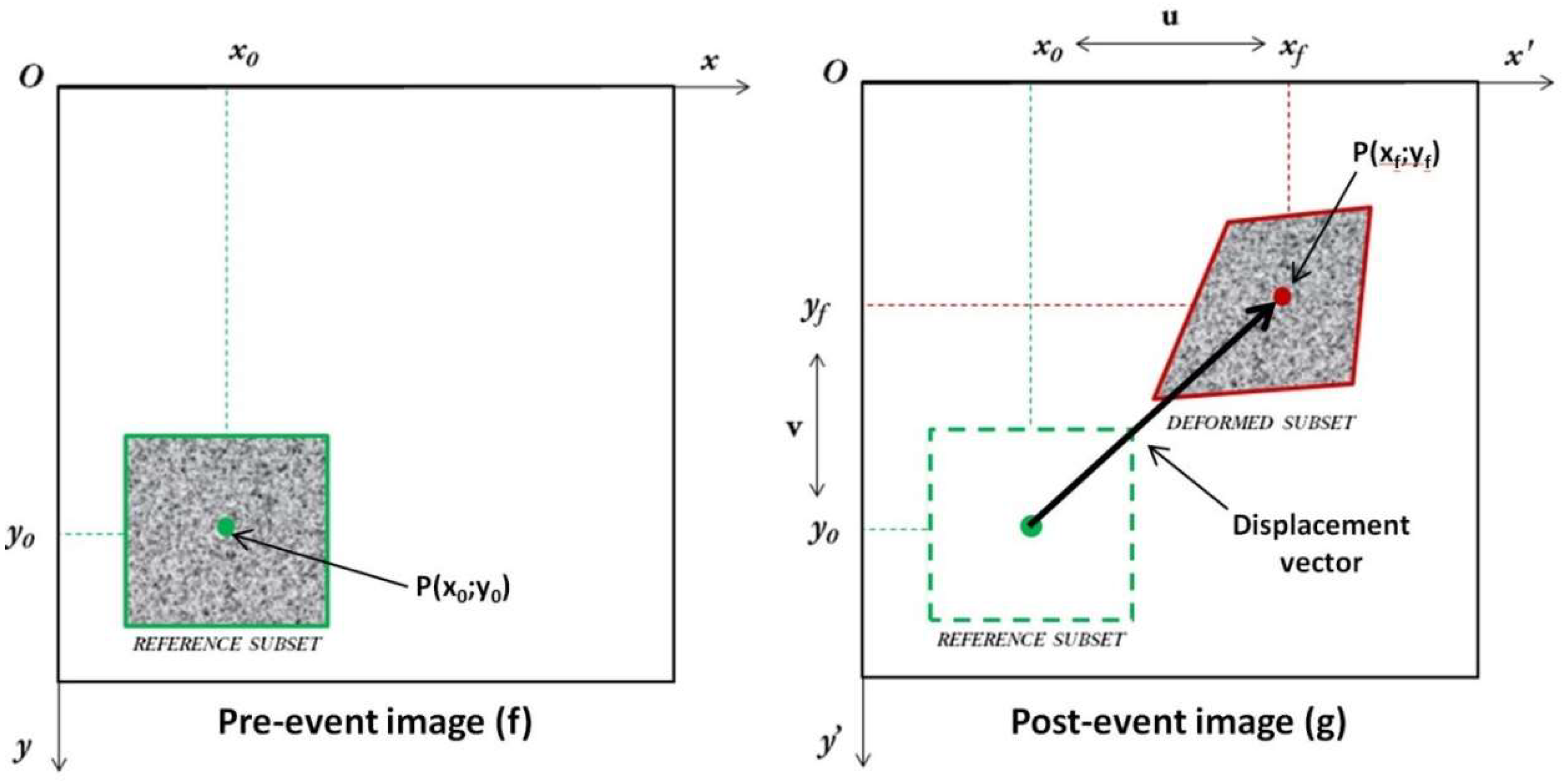
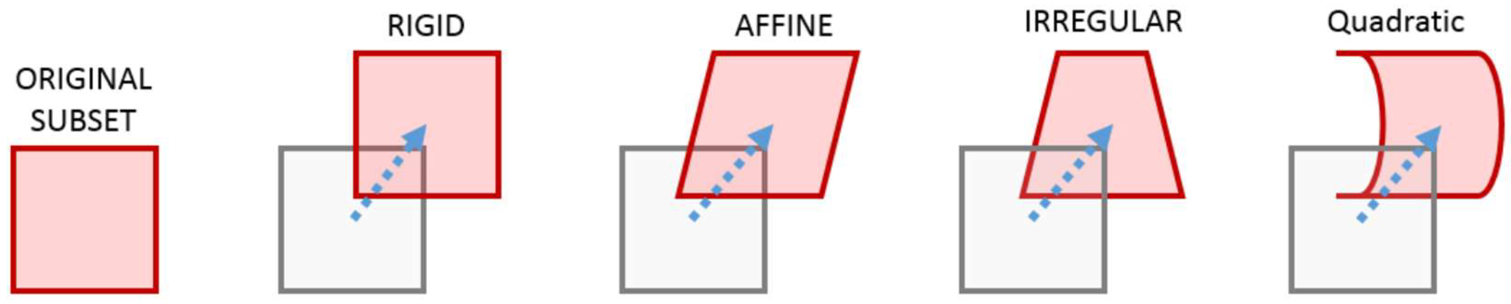
2. Basic Principles of Digital Image Correlation (DIC)

According to the author of [44], several digital approaches can be used to analyze and manipulate available imagery datasets, and different types of information can be extracted depending on the typology of the chosen image processing technique. Basically, digital image processing techniques are founded on the extraction of ground change information via comparisons between different types of images (e.g., satellite-based, airborne or ground-based imagery) collected at different times over the same area and scene.
DIC is an optical-numerical measurement technique that can provide full-field 2D surface displacements or deformations of any type of object. Deformations are calculated via comparisons and processing of coregistered digital images of the surface of the same “object” collected before and after the deformation event [45]. In most cases, the DIC technique allows for displacements/deformations to be measured without the installation of sensors/reflectors in the measured object; i.e., it can be considered to be a fully remote measurement system [46]. However, the basic requirement for DIC analyses is the occurrence of a random speckle pattern on the object’s surface, which is essential for obtaining a unique solution in the correlation process. Essentially, identifying the correspondence between single pixels in two images is impossible because the intensity value of a single pixel can typically be found in thousands of other pixels in the post-event image. Consequently, unique correspondence does not occur [47]. Therefore, consistency between two speckle patterns is accomplished by considering a pixel and its neighborhood in the pre-event image (ƒ) and searching for the same subset in the post-event image (g) (Figure 1). The size of the subset depends on the granularity of a non-repetitive, isotropic, high-contrast pattern (denoted as the speckle pattern) [48].
Hence, the correlation processes have to refer to a region of interest (ROI). The ROI represents an area of the picture chosen by the operator, and it is overlaid only on the object to be correlated. Therefore, between the reference and the deformed images, the ROI represents the analysis mask in which the correlation algorithm operates. Caution must be exercised when selecting the subset size. According to the authors of [49,50,51], the chosen optimum subset size must not be too small and is governed by the granularity of the speckle pattern. A subset that is too large, however, cannot be used to describe large heterogeneous deformations and will substantially worsen the sub-pixel accuracy. Therefore, to guarantee a reliable displacement measurement, the subset has to be chosen depending on the typology of the performed images, because the typology can lead to high sub-pixel accuracy measurements for images with larger contrasts. Furthermore, the step size, which is the shift of the subset during the correlation process, has to be set carefully. Generally, the subset size should at least have the dimensions of the largest blob appearing in the speckle pattern [52]. This procedure is repeated for a grid of pixels spaced at regular intervals (step size). The information density is increased when the step size is small.
Several functions are used to match the subset from the pre-event image to the post-event image. As reported in Reference [53], one function is the magnitude of intensity value difference,
  R ( x ,   y ,   x * ,   y * ) =   Σ   | F ( x ,   y , ) G ( x * ,   y * ) |  
and another function is the normalized cross-correlation (NCC),
  N C C ( x ,   y ,   x * ,   y * ) = F ( x ,   y ) G ( x * ,   y * ) F ( x ,   y ) 2 G ( x * ,   y * ) 2  
where F(x, y) and G(x*, y*) represent the intensity values within the subset of the pre-event and post-event images, respectively; (x, y) and (x*, y*) are the coordinates of a point on the subset before and after deformation, respectively; and the symbol Σ represents the sum of the values within the subset. The coordinate (x*, y*) after deformation is related to coordinate (x, y) before deformation. Hence, the displacement components are obtained by determining the best setting of the coordinates after deformation (x*, y*) that minimize or maximize the R or NCC parameters [53].
The subset chosen for the DIC analysis has to be tracked in the post-event images. The subset shape during the entire correlation process must be able to change its geometrical parameters (such as its size, profile and position). Different numbers of parameters define the method by which the subset can deform during the correlation process. If the first-order partial derivatives are considered, the general form of an affine transformation is retrieved. The affine transformation accounts for rigid body motion (translation and rotation), shear and normal stretching. Next, by adding the terms Δx and Δy, an expression similar to that of a four-node bilinear Lagrange interpolation function in a finite element analysis is yielded and mapping onto an irregular quadrangle deformation is allowed. Finally, second-order terms can be included in the shape function to introduce the effects of full bending of the subset [52] (Figure 2).
In the case of a robust and homogeneous deformation, an affine transformation order and a large subset will be able to describe the deformation process. When the deformation is more complex and heterogeneous, smaller subset sizes should be used or a higher transformation order needs to be introduced for a precise description of the deformation process.
Most of the DIC algorithms use a subset-based scanning method to measure the displacements, thereby allowing for spatially continuous deformation detection with sub-pixel accuracy [54]. The same approach can be applied with only two images or when using stacks of images collected at different times, thereby achieving time series of deformations.

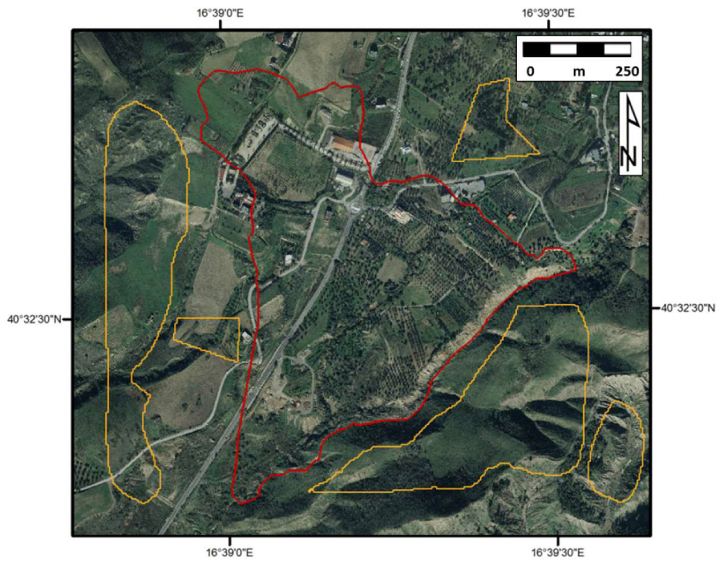
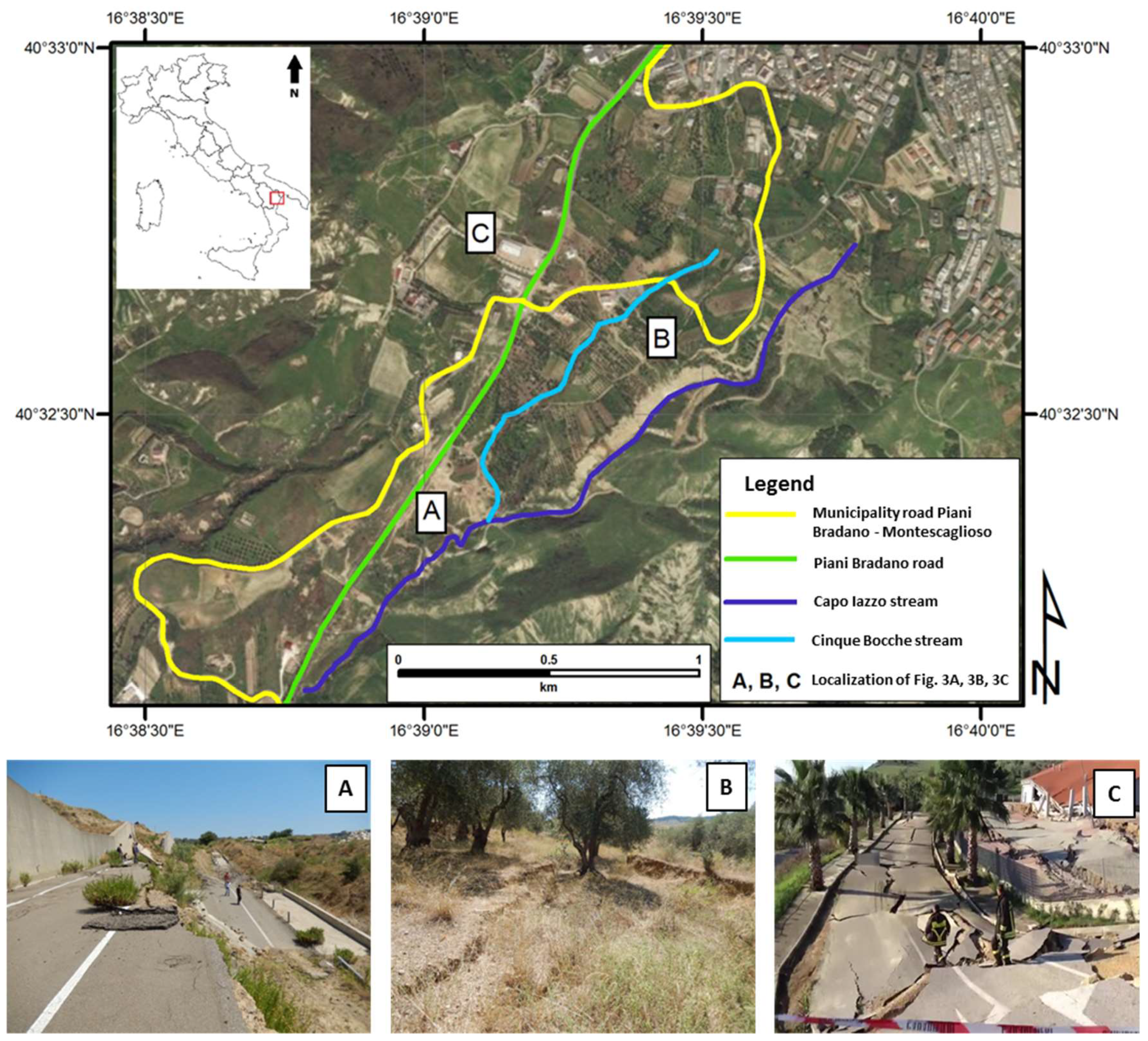
3. 3 December 2013 Montescaglioso Landslide

Montescaglioso (Basilicata region, Southern Italy) is a small village located on a hilltop at approximately 350 m a.s.l. along the left bank of the Bradano River. Based on the peculiar concave shape of the Montescaglioso relief, which illustrates an actively changing morphology, several types of ground evidence can be detected, such as inactive ancient landslide bodies, scarps and relicts, and blocks [23,38,39,41,42,43,55].
On 3 December 2013, a huge landslide occurred that damaged commercial buildings, infrastructure and private houses (Figure 3). The SW-directed slope instability affected part of the Montescaglioso hill. According to the authors of [43], the landslide covered an area that was approximately 500,000 m2, mobilized nearly 8 million m3 of material, and had a presumed failure surface at an approximate depth of 40 m.
The landslide involved an area spanning from 200 to 100 m a.s.l., and had a total length of approximately 1200 m and a width of approximately 800 m. The intense and persistent rainfall that affected southern Italy between 5 October and 8 October 2013, and between 30 November and 2 December 2013, has been considered the main trigger for the landslide event [23,38,39,41,43,55].
During the complex evolution of the 3 December 2013 Montescaglioso landslide, evidence of ground failures was collected starting at 1:00 p.m. CET on the same day. Consequently, according to the authors of [38], the deformation reached the lower left flank of the landslide, generating several scarps and counter-scarps characterized by lengths of a few tens of meters and maximum heights of 7–8 m. Then, the movement involved the municipality road Piani Bradano and progressively evolved toward the SE, thereby affecting the area on the right bank of the Capo Iazzo stream. In an additional phase, the instability involved the NW sector of the slope [39] (Figure 3). The last phase of the movement (occurring on the night between 3 and 4 December 2013) was typified by a retrogressive style that caused a northward replacement of the landslide area. According to the landslide classification introduced by the authors of [56] and highlighted by the authors of [38,39,42], the slope instability has been considered a rapid complex earth slide [1.8 m/h ≤ velocity <3 m/min]. Indeed, most of the movement occurred within a period of approximately 15–20 min, with peaks in velocity of approximately 0.75 m/min corresponding with certain sectors.
In the frame of this work, a specific field survey aimed at better constraining the deformational pattern and mapping the main geomorphological features of the slope was performed in July 2016. The main focus during the field survey was to observe and describe those geomorphological features caused by recent and previous slope instability processes.
Moreover, the field survey activities allowed for the reconstruction of the kinematic evolution of the Montescaglioso landslide by identifying all of the slope sectors involved in the 3 December event. As shown in Figure 3A–C, local infrastructure, buildings and private fields were seriously damaged and visually displaced. The occurrence of wide and deep ground tension cracks, and all of the new geomorphological features in the sectors highlighted in Figure 3, were used to improve the calibration and definition of the landslide boundary compared with the previous delineations in References [38,41]. Subsequently, based on photo-interpretative observations and terrain analyses performed in a Geographic Information System (GIS) environment, the triangular-shaped boundary of the Montescaglioso landslide has been defined, as previously suggested by the authors of [38,41].
The extensive and complex deformational pattern provides insights on the kinematic behavior of the landslide, and the geological and geomorphological constraints [23], and provides a valuable opportunity for testing the potential of the DIC technique by exploiting the different image datasets available.

4. Materials and Methods

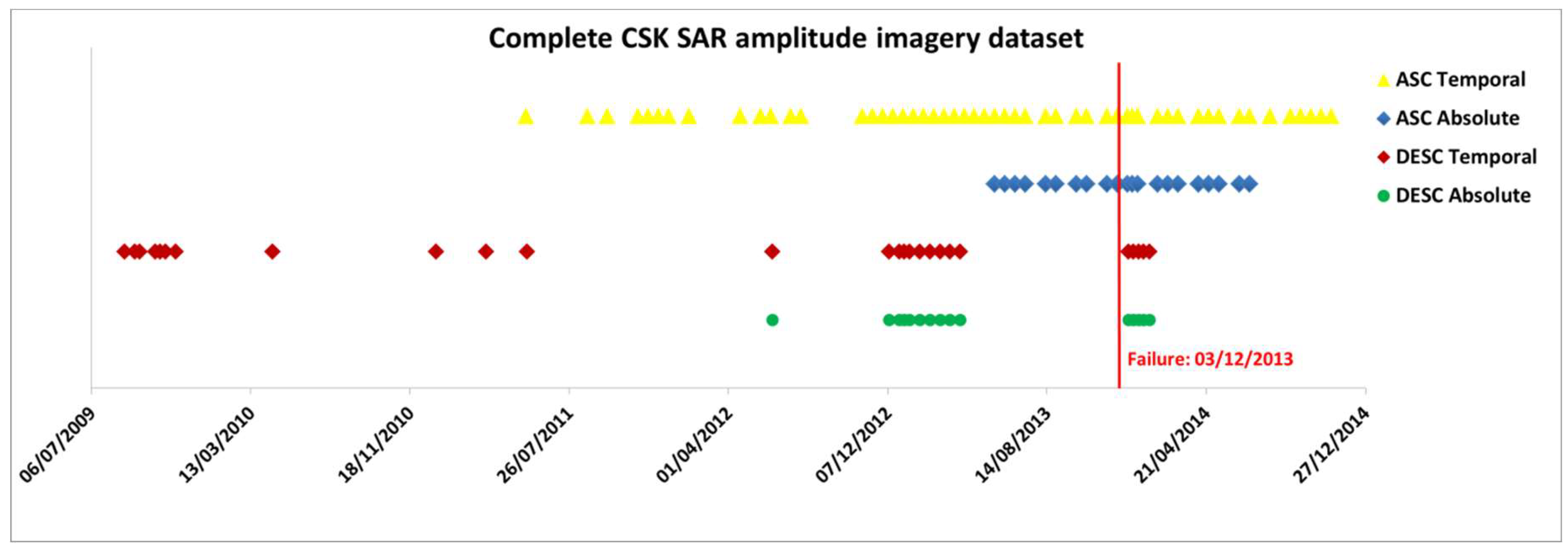
4.1. Available Datasets

An extensive examination of the datasets suitable for DIC analyses was conducted in the first step of the study, via an examination of the International Space Agency’s satellite image databases and national/regional databases of DTM and aerial images. Among the remotely sensed datasets, all images with a suitable geometric resolution and pre-post event images were chosen:
-
COSMO-SkyMed SAR Images (in both ascending and descending geometry);
-
LANDSAT 8 OLI-TIRS Images;
-
DTM; and,
-
High-resolution Aerial Optical Images.
The complete COSMO-SkyMed (CSK) dataset includes 60 SAR amplitude images in ascending geometry that were acquired between May 2011 and May 2015, and 28 SAR amplitude images in descending geometry that were collected between August 2009 and May 2015 (Figure 4). All images were collected in StripMap HIMAGE acquisition mode, and their ground-range and azimuth resolutions are approximately 3 m. According to Reference [8], because of its side-looking acquisition mode, SAR images are subjected to geometrical distortions. The types of areas that are affected by overlays or shadows cannot be imaged by the sensor [57]. In fact, the topography and, more precisely, the local slope along the line of sight (LOS) of the satellite can generate distortions. Hence, a method of overcoming this limitation is to combine ascending and descending orbits over the same area.
The LANDSAT 8 OLI-TIRS dataset includes two panchromatic images (with 15 m nominal resolution) acquired on 26 October 2013 (LC81880322013299LGN00) and 15 February 2014 (LC81880322014046LGN00).
The high-resolution (HR) aerial optical image dataset includes two orthophotos collected in July and December 2013 (i.e., before and after the landslide failure) respectively, with similar geometric resolutions; i.e., 0.3 m/pixel and 0.2 m/pixel for the pre-failure and the post-failure images, respectively.
Furthermore, through two airborne LiDAR surveys performed by local authorities before and after the failure, two high-resolution DTMs (1 × 1 m cell size) were collected in July and December 2013, respectively.
A synopsis of the available datasets is shown in Table 1, which provides a description of the platforms used, the types of sensors, the nominal geometric resolutions and the dates of image collection.

4.2. Image Processing Tools

Considering the extensive and heterogeneous image datasets available, different tools were used for the image pre-processing and then for the DIC analyses. The pre-processing phase is required to prepare the pre-post image pairs from each single dataset for processing using DIC software. The following software tools were used:
-
ENVI® v. 5.4 (Environment for Visualizing Images) [58]: ENVI® was used to visualize the available dataset and perform oversampling of both aerial orthophotos to 0.8 m/pixel geometric resolution (by using the nearest-neighbor interpolation method);
-
ESRI ArcGIS [59]: This software performs a number of surface operations and generates eight shaded reliefs before performing the DIC analysis on the pre-post DTM pair; and,
-
SARPROZ© (SAR PROcessing tool by periZ) [60]: This tool was used to perform time-averaged filtering on the entire CSK SAR amplitude dataset (in both ascending and descending geometries).
The DIC analyses were undertaken using two open source software programs: COSI-Corr and GOM Correlate.
-
COSI-Corr (Co-registration of Optically Sensed Images and Correlation) [61] is a sub-pixel image correlation algorithm (developed by the authors of [62,63] that is available as an open-source plug-in for the ENVI® software package. According to References [33,54,62,64,65], to allow for displacement measurements, an initial parameter setting has to be chosen as follows: (i) a window size, which is the size in pixels of the patches that will be correlated in the x and y directions; (ii) a step, which determines the step in the x and y directions in pixels between two sliding windows; and (iii), the type of correlator engine to be chosen, between frequency (Fourier based) and statistical typology. Further detailed descriptions of the algorithms and characteristics of this software are available in References [62,66].
-
GOM Correlate [67] is a DIC evaluation software program used for materials research and component testing. GOM Correlate software is based on a parametric concept that forms the underlying foundation for every single function [68,69]. This parametric approach ensures that all process steps are traceable, thereby guaranteeing process reliability for measuring results. In addition, in GOM Correlate, parameters must be initialized. While establishing the surface component, the software finds square-shaped facets in the collected scenes. Basically, the square facets, set in GOM Correlate, are equivalent to the subset, set in COSI-Corr analyses. GOM Correlate software identifies these facets by the stochastic pattern quality structure. The distance between the individual square shapes has to then be properly set. The point distance describes the distance between the center points of the adjacent square facets. This setting influences the measurement point density within the surface component. The measurement point density increases as the point distance decreases. A higher spatial resolution is obtained by decreasing the distance between the facets [68,69].
In References [54,69], the DIC analyses were performed by using adaptive approaches, providing the image correlation through the iterative least squares algorithm.
Here, the main requirements were that this correlation method is quite robust against noise and allows measurements with sub-pixel accuracy, by sliding a window scanning the pre- and post-event images [54]. Hence, the measurements of the movements at a sub-pixel scale were possible by estimating the bicubic interpolation [54,69].
Finally, statistical analyses were performed using ENVI® and the Image Processing Toolbox in MATLAB v. R2017b [70].
Further detailed descriptions of the algorithms and technical specifications of the above-mentioned software are available on the official websites.

5. Data Analyses and Results

The data analyses consisted of two main phases: image pre-processing, which was performed to prepare the image pairs for processing; and the DIC data analyses, which were performed to infer information on the ground deformation and for statistical analyses of the accuracy of the measurement method.

5.1. Image Pre-Processing

For each dataset, a number of pre-processing operations were needed to correct, co-register, better define and filter the pre-post image pairs.
To better calibrate and validate the DIC analyses performed on the absolute SAR amplitude images, a temporal average filtering process was applied to the available ascending and descending CSK datasets (Figure 4 and Figure 5). Hence, the environmental and instrumental background noise has been significantly decreased, leading to an increase in the effective signal. In this way, the signal-to-noise ratio (SNR), related to the horizontal displacement field measurement and estimation, has been increased as highlighted in Reference [39].
Regarding the DIC analyses performed on the pre-post DTMs, a number of surface operations were performed in the GIS environment, and eight shaded reliefs were generated. The procedure was characterized by the sun-azimuth angle variation in steps of 45 degrees, with contemporary maintenance of the sun-altitude angle at 45 degrees. The DIC analysis was based on the correlation of the different combinations of the hillshade raster data. According to the authors of [33,71], a COSI-Corr analysis has a higher probability of success for retrieving high-quality displacement results if the correlations are based on the shaded DSMs (or DTMs).
The US Geological Survey’s Earth Resources Observation and Science (EROS) Center [72] directly radiometrically corrected and coregistered the LANDSAT 8 OLI-TIRS images to a cartographic projection with rectifications for terrain displacement, thereby resulting in a standard orthorectified digital image. More information is available on the official website.
Finally, both HR aerial optical orthophotos were oversampled at a 0.80 m/pixel geometric resolution because of their different initial geometric resolutions.

5.2. DIC Analyses

A sensitivity study was performed on the application of the DIC technique to different datasets to test the potentialities and limitations, and the displacement of the Montescaglioso landslide area was calculated using all the available datasets.
Alternately, both DIC software programs described in Section 4.2 were used for each dataset to ensure the mutual control of the displacement measurements, define the movement directions and assess the background noise. The latter represents a fundamental parameter because it allows for a precise quantification of the environmental and instrumental/sensor errors.
Because the available processed datasets are characterized by regular and repetitive temporal resolutions, an in-depth study of the background noise with a high degree of reliability was undertaken for the entire imagery dataset. Furthermore, specific background/instrumental errors were assigned based on the collecting sensor (CSK, LANDSAT 8 OLI-TIRS, airborne LiDAR and aerial camera).

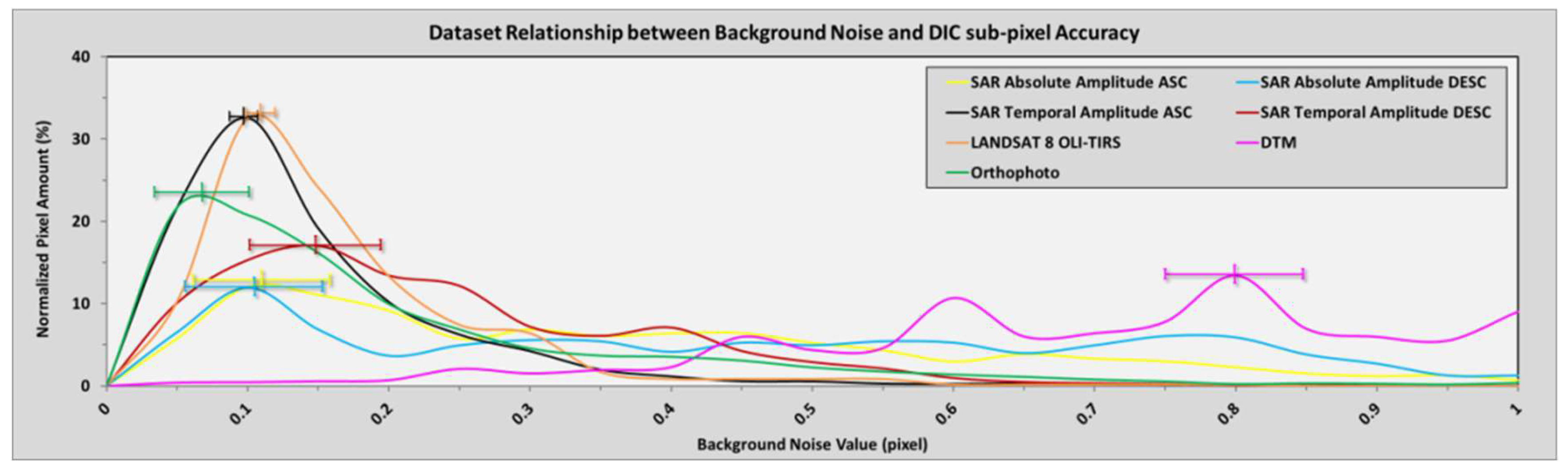
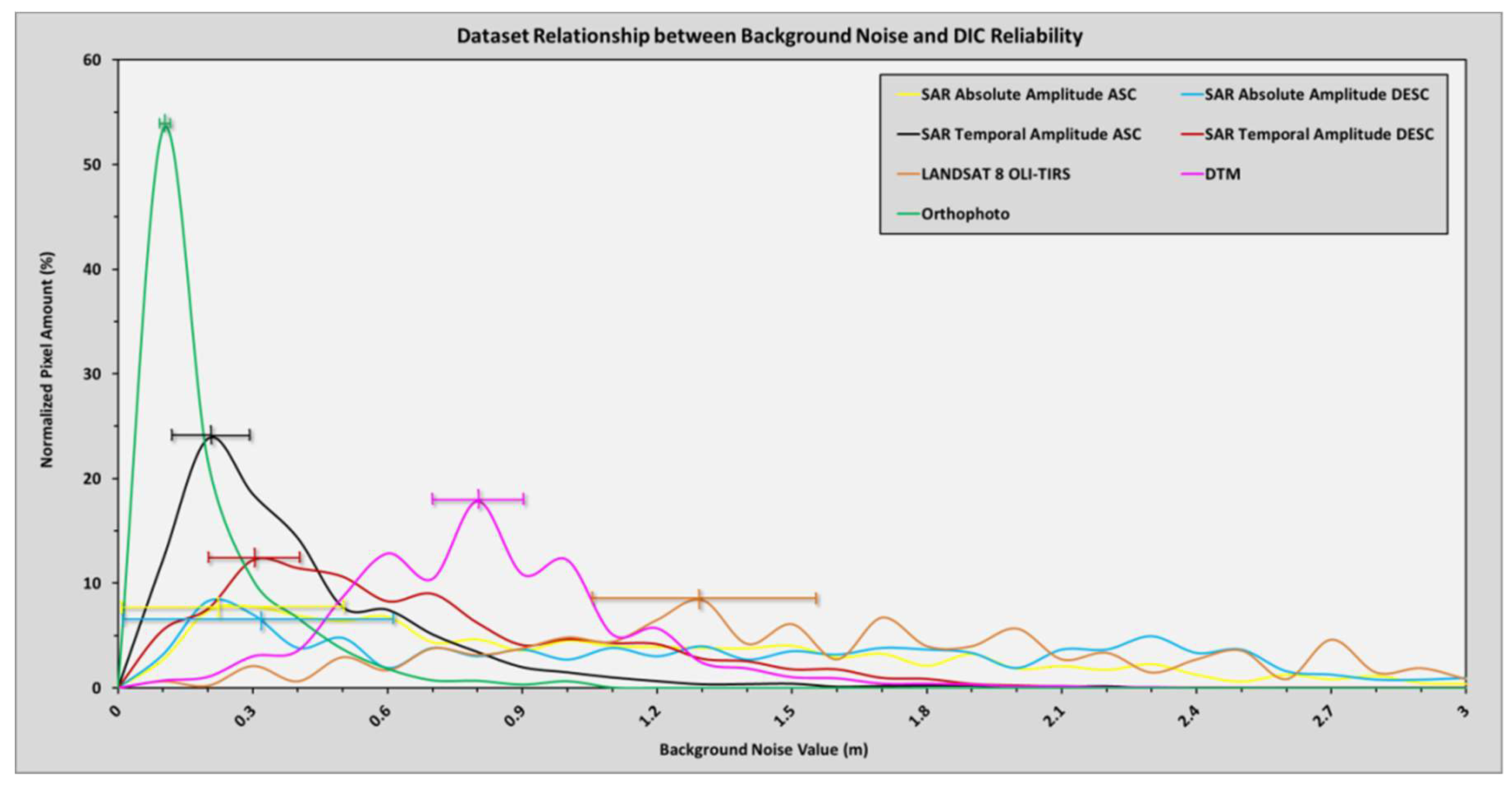
5.2.1. Analyses of the Background Noise

Because the surrounding sectors of the Montescaglioso area were unaffected by the general movement of the slope failure (i.e., they were not affected by any type of displacement), they were subjected to a DIC analysis to assess the background noise.
To that aim, a methodological analysis based on two different region of interest (ROI) approaches was conducted.
In approach #1, equivalent ROIs were designed in the surroundings of the Montescaglioso landslide using the DTM’s footprint (i.e., the smallest one) as a general reference for the entirety of the datasets (Figure 6), thereby reducing any ROI-related uncertainty. Through this approach, the background noise for each dataset was estimated and consistent measurements were therefore obtained.
In approach #2, different ROIs were selected in the surroundings of the Montescaglioso landslide using the overall footprint of each dataset as a reference, thereby accounting for the different geometric resolutions of the data. In this way, the analyses were performed on different areas for each dataset to achieve different background noise estimations, and the results indicated different sources of error (Figure 7, Table 2).
In both approaches, the measured background noise values were estimated. A comparison of the results (Table 2) showed similar findings within a small error fraction, which may be related to the unconstrained choice of the ROI selections in the same areas and differences in the geometrical and temporal resolutions.

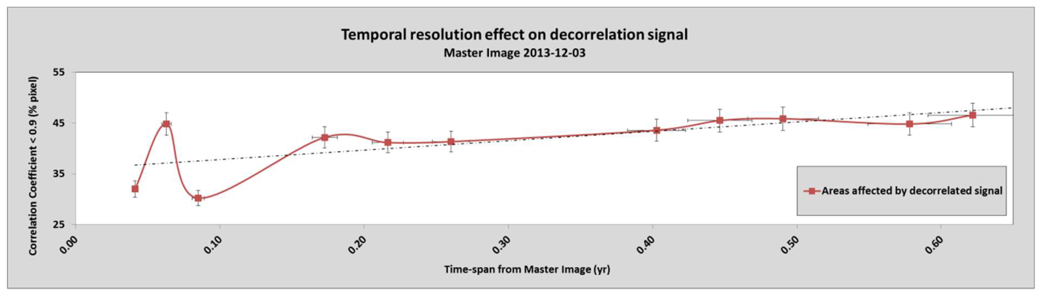
5.2.2. Analyses of the Temporal Resolution Effect

The regions of the processed imagery affected by the temporal resolution were similar to those affected by a low SNR. This matter was investigated through an analysis of the ascending CSK SAR absolute amplitude dataset. In Figure 8, the gradual intensification of the spatial extent of the decorrelated signal is shown. An analysis and comparison of the available images among the datasets showed that the random speckle pattern, a feature of the SAR absolute amplitude images, was always affected by different gray levels and tonal degrees. In fact, because of the different data collection times, the areas surrounding the Montescaglioso slope were characterized by important gray level, texture and tonal changes unrelated to ground movement.
Specifically, by using the ascending CSK SAR absolute amplitude dataset and analyzing the same ROIs previously used in the background noise estimation (specifically in approach #1) (Figure 6), a strategy has been adopted. With the aim of evaluating the percentage increase of the sectors affected by a decorrelated signal during the period, the DIC analyses performed between the last pre-failure image (3 December 2013, as the master image) and a number of post-failure images (from 18 December 2013 to 28 June 2014, as slave images) were considered (Figure 9, Table 3).

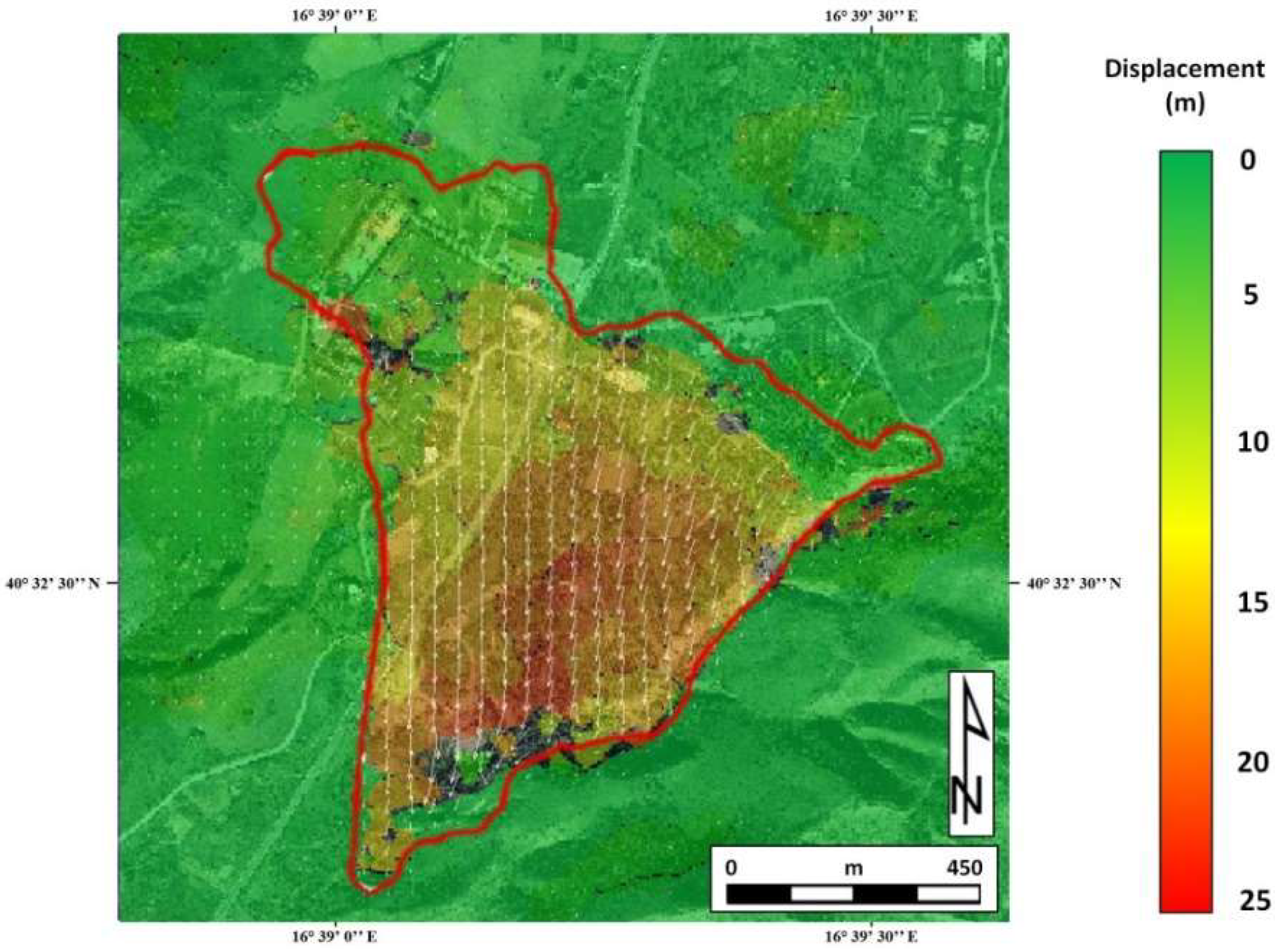
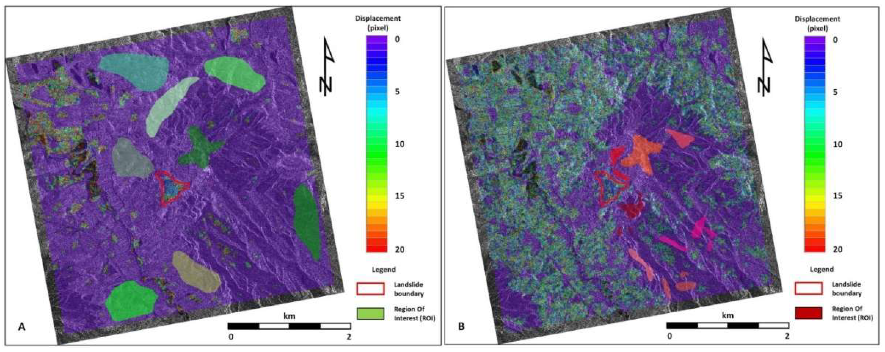
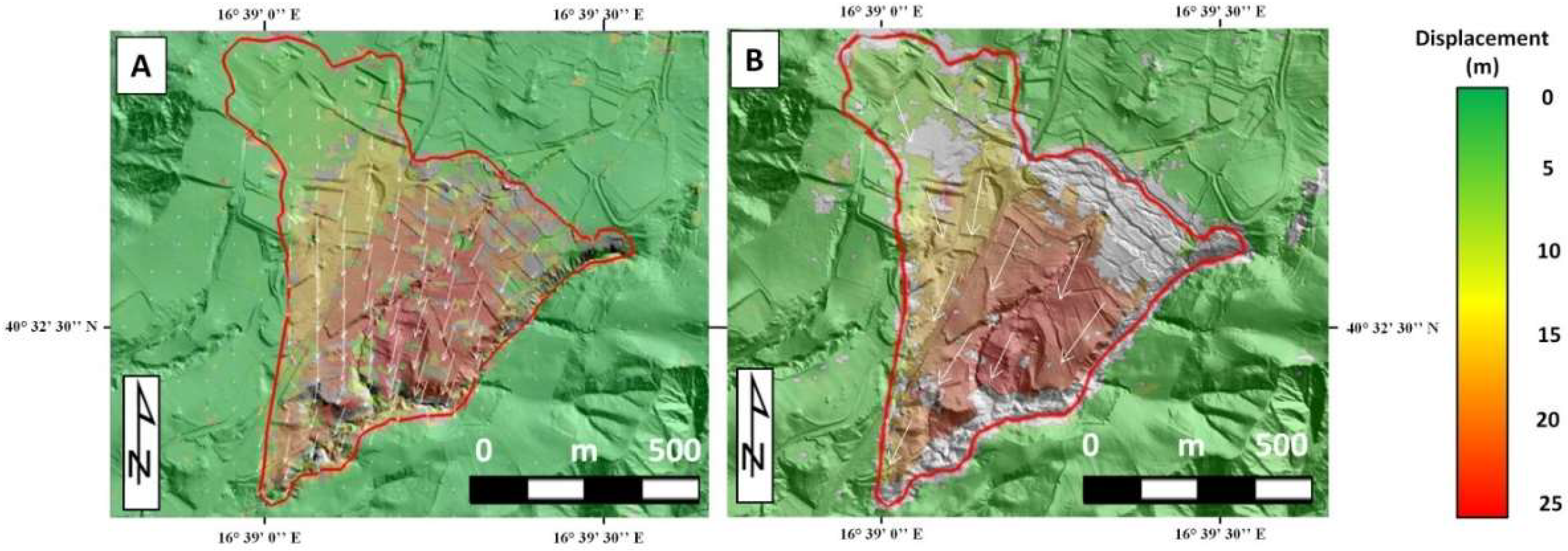
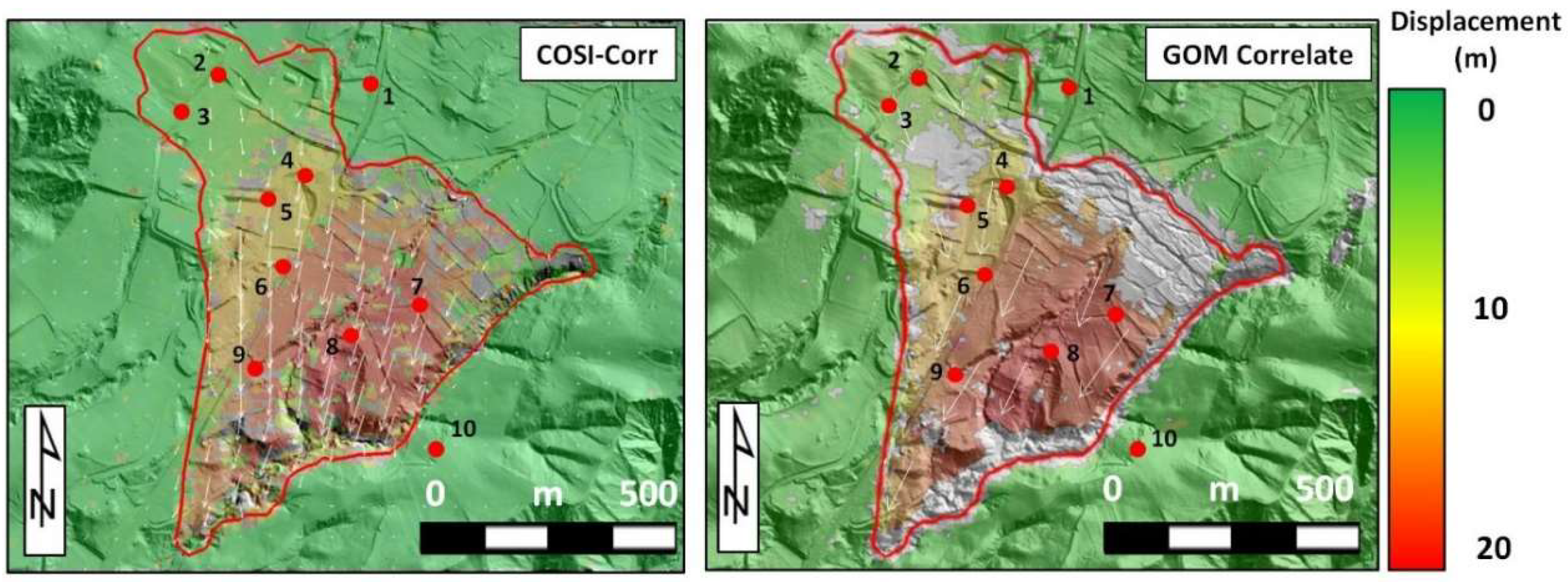
5.2.3. Analyses of the Landslide Deformation

The deformation of the Montescaglioso landslide area (Figure 6) was measured for each dataset shown in Table 1 using both the COSI-Corr and GOM Correlate software, setting a correlation threshold of 0.9. The best parameters for use in each analysis were identified through a trial and error approach, and the results are shown in Table 4.
Displacement maps of each analysis are reported in the following figures, except for the descending CSK SAR absolute amplitude dataset, which is characterized by a moderate percentage of areas affected by the decorrelated signal and is hence unrepresentative (Figure 10, Figure 11, Figure 12, Figure 13, Figure 14 and Figure 15).
The displacement pattern of the Montescaglioso landslide was inferred from an analysis of Figure 10, Figure 11, Figure 12, Figure 13, Figure 14 and Figure 15. All the processed maps show that the amount of displacement increases from the NW sector (~2–3 m) to the central part of the landslide and the toe, and the value is as large as 20–21 m. Moreover, similarities are observed in the amount of movement as well as in the direction of the landslide displacement field. In fact, the inferred vector fields show a direction that is generally towards the S-SE in the NW sector but S-SW in the NE sector, thus reaching a prevalent SW direction in the central portion.
In Figure 10, Figure 11b and Figure 14b, certain portions of the NE and E sectors of the landslide are characterized by a lack of signal where any type of results can be retrieved. In the areas immediately surrounding the landslide, no movement has been registered as shown by the green tones in each DIC displacement map.

6. Discussion

By taking advantage of a large dataset of pre- and post-failure images of the 3 December 2013 Montescaglioso landslide, an extensive sensitivity analysis using DIC has been performed. In addition to the evaluation of the landslide displacement pattern, this work provided insights into the reliability and accuracy of the DIC methodology for landslide investigation and monitoring purposes.
For most of the analyses, the percentage of the landslide area with a good correlation (i.e., where reliable deformation values can be derived) exceeded 70% of the available pixels, thereby providing a comprehensive overview of the landslide deformation field.
The landslide deformation field was quite consistent among the different datasets and the different data processing techniques used in this paper, thus demonstrating the reliability of the measurement technique. Furthermore, by selecting a correlation threshold of 0.9, the results are similar to those available in the literature [38,39,41,42,43,55,73,74,75,76], as well as the evidence inferred from field inspections. Figure 16 and Table 5 show the comparative results between the analyses performed using the COSI-Corr and GOM Correlate software for the same dataset. An analysis of the corresponding pixels (Table 5) showed that the average discrepancy was less than 0.2 pixels, with the differences ranging from 0.07 to 0.54 pixels.
Nevertheless, although GOM Correlate provided good results for a few datasets, COSI-Corr software was able to process all the available datasets (Table 6).
An analysis of portions of the slope not affected by the 3 December 2013 landslide was performed to estimate the sub-pixel accuracy and the environmental and instrumental background noise affecting each dataset, as previously performed by several authors [8,31,35,62,63,64,65,77,78,79,80,81,82,83,84].
The background noise values (in pixels for Figure 17 and in meters for Figure 18) were calculated for each dataset using COSI-Corr software. Specifically, each curve represents the percentage of pixels (on the y-axis) characterized by different values of background noise/displacement accuracy (on the x-axis) for each dataset, thereby showing the most likely background noise value (i.e., the value corresponding to the highest percentage on the y-axis). Moreover, to better estimate the standard deviation of the background noise value, a window (i.e., background noise interval) corresponding to an overall percentage of pixels equal to 30% was calculated for each curve.
Focusing only on the two end members, LANDSAT 8 OLI-TIRS is characterized by a displacement accuracy of approximately 1/10 of a pixel, whereas the shaded DTM dataset is characterized by a displacement accuracy of approximately 8/10 of a pixel (Figure 17). However, if the different pixel sizes of the two datasets (i.e., 15 m for LANDSAT OLI-TIRS and 1 m for the shaded DTM) are accounted for, better accuracy is achieved for the DTM dataset (i.e., 0.8 m) than for the LANDSAT OLI-TIRS dataset (i.e., 1.3 m) (Figure 18).
For the 30% reliability windows, high variability between the different datasets can be observed, and is likely caused by the different image resolutions; i.e., geometric, radiometric and spectral [85]. For example, by only focusing on the two end members, we can see that the orthophoto dataset is characterized by a reliability window of approximately 0.05 m, whereas the LANDSAT OLI-TIRS dataset is characterized by a reliability window of 0.9 m (Figure 18).
Moreover, strong differences are observed between the results, with absolute SAR images and temporal average amplitude images, both in terms of noise value and reliability windows especially (Figure 17 and Figure 18). Such a difference is caused by the despeckling of SAR images achieved by averaging several images acquired at different times as also shown in Figure 5 [86,87,88,89,90].
The availability of an ascending stack of CSK SAR absolute amplitude images allowed us to also investigate the temporal decorrelation that affected certain sectors in the surrounding areas of the Montescaglioso landslide. As shown in Figure 8 and Figure 9, the time span between the processed images increased from 15 days to over 200 days, which caused an increase of the decorrelated area from approximately 32% to 46%. The temporal resolution of remotely sensed data may also affect the precision and accuracy of the measurements and analyses performed [91]). According to the authors of [8,92], the time span between two image acquisitions can play an important role in increasing the decorrelated signal [93]. However, in most cases, the time resolution is governed by the data collection procedure (e.g., different satellite revisit times), thus ensuring a significant impact on all types of measurements [94]. Therefore, a compromise has to be found between the correlation loss and the minimum signal detection. For example, with slow landslides, the time span between the two acquisitions has to be large enough to detect the signal, but also needs to be short enough to avoid decorrelation [8,92,95].
The above findings indicate that landslides characterized by fast movements and/or episodic occurrences might be more successfully investigated by employing amplitude-based techniques (such as the DIC) than interferometric-based analyses, because the movement may induce important changes in the surface topography. In fact, when a large ground displacement between two SAR images collected at different times in the same geometry is too large to be measured by interferometry (InSAR), image-based techniques, such as mainly the sub-pixel image-correlation method, can be particularly suitable, complementary and successful [37,96,97,98,99,100,101,102,103,104,105,106,107,108,109,110,111].

7. Conclusions

The aim of this work was to verify the efficacy and sensitivity of the DIC technique for landslide displacement measurements. For that purpose, the kinematic behavior of the 3 December 2013 Montescaglioso landslide was investigated, using different remotely sensed imagery and different data processing software.
The measured displacement values, achieved with all the available processed datasets (e.g., LANDSAT 8 OLI-TIRS, high-resolution airborne optical ortho-photos, DTMs and COSMO-SkyMed SAR imagery), range between a few meters (2–3 m) in the NW sector of the landslide body and up to 20–21 m in its central portion, consistent with the results attained by other authors, both in terms of displacement magnitude and direction [38,39,40,41,42,43,73,74,75,76].
A detailed study in areas not involved in the landslide movement was performed to estimate the environmental-instrumental background noise in terms of pixel and meters values, and comparisons of the results obtained from the different datasets and software were performed.
The maximum achieved accuracy values for the pixels and displacements are on the order of 0.1 pixels and 0.1 m, respectively. The different datasets show different sub-pixel accuracies (8/10 of a pixel referred to the DTM results, 1/10 of a pixel for the ortho-photos and between 1/10 and 2/10 of a pixel for the CSK absolute and temporal amplitude SAR imagery), as well as different reliability windows, thereby demonstrating the importance of the dataset characteristics on the final results of the analyses.
Specifically, the LANDSAT 8 OLI-TIRS results indicate that the radiometric and geometric resolutions of the images have different impacts. The LANDSAT 8 OLI-TIRS images are characterized by one of the best sub-pixel accuracies (1/10 of a pixel) because of their high radiometric accuracy; however, because of the low nominal geometric resolution (i.e., 15 m), the achieved background noise value is on the order of 1.4 m.
The Montescaglioso landslide is a case in which the availability of different datasets and the irregular patterns of ground deformation have provided ideal conditions for successfully testing the sub-pixel image correlation technique and demonstrating the potential use of this technique as an investigation/monitoring tool for landslides.
The results achieved shed light on the potential of the herein proposed DIC approach for landslide monitoring, because of its capabilities to be applied at different spatial and temporal scale, to a variety of landslides. Furthermore, the rapidly increasing geometric, radiometric and temporal resolution of optical sensors could reduce most of the present limitations of such a methodology (e.g., limited displacement accuracy and low data sampling rate), especially if combined with the growing data processing capabilities of high performance computing.

Author Contributions

Conceptualization, P.C. and P.M.; methodology, P.C. and P.M.; validation, P.C. and P.M.; formal analysis, P.C.; investigation, P.C.; data curation, P.C., P.M and F.B.; writing-original draft preparation, P.C.; writing-review and editing, P.C., P.M. and F.B.; visualization, P.C., P.M.; supervision, P.M. and F.B.

Funding

The founding sponsors had no role in the design of the study; in the collection, analyses, or interpretation of data; in the writing of the manuscript, or in the decision to publish the results.

Acknowledgments

The authors would like to thank the Italian Space Agency (ASI) for providing the COSMO-SkyMed SAR images, and local authorities for the DTMs and aerial optical orthophotos used in this study.

Conflicts of Interest

The authors declare no conflict of interest.

References

  1. Alexander, E.D. Vulnerability to landslides. In Landslide Hazard and Risk; Glade, T., Anderson, M.G., Crozier, M.J., Eds.; John Wiley & Sons, Ltd.: New York, NY, USA, 2004; pp. 175–198. [Google Scholar]
  2. Kjekstad, O.; Highland, L.M. Economic and social impacts of landslides. In Landslides—Disaster Risk Reduction; Sassa, D., Canuti, P., Eds.; Springer: Berlin, Germany, 2008; pp. 573–587. [Google Scholar]
  3. Sanchez, C.; Lee, T.-S.; Young, S.; Batts, D.; Benjamin, J.; Malilay, J. Risk factors for mortality during the 2002 landslides in Chuuk, Federated States of Micronesia. Disasters 2009, 33, 705–720. [Google Scholar] [CrossRef] [PubMed]
  4. Petley, D. Global patterns of loss of life from landslides. Geology 2012, 40, 927–930. [Google Scholar] [CrossRef]
  5. Baroň, I.; Supper, R. Application and reliability of techniques for landslide site investigation, monitoring and early warning—Outcomes from a questionnaire study. Nat. Hazards Earth Syst. Sci. 2013, 13, 3157–3168. [Google Scholar] [CrossRef]
  6. Mantovani, F.; Soeters, R.; Van Wasten, C.J. Remote sensing techniques for landslide studies and hazard zonation in Europe. Geomorphology 1996, 15, 213–225. [Google Scholar] [CrossRef]
  7. Delacourt, C.; Allemand, P.; Casson, B.; Vadon, H. Velocity field of the “La Clapiere” landslide measured by the correlation of aerial and QuickBird satellite images. Geophys. Res. Lett. 2004, 31, L15619. [Google Scholar] [CrossRef]
  8. Delacourt, C.; Allemand, P.; Berthier, E.; Raucoules, D.; Casson, B.; Grandjean, P.; Pambrun, C.; Varel, E. Remote-sensing techniques for analysing landslide kinematics: A review. Bull. Soc. Géol. Fr. 2007, 178, 89–100. [Google Scholar] [CrossRef]
  9. Voigt, S.; Kemper, T.; Riedlinger, T.; Kiefl, R.; Scholte, K.; Mehl, H. Satellite Image Analysis for Disaster and Crisis-Management Support. IEEE Trans. Geosci. Remote Sens. 2007, 45. [Google Scholar] [CrossRef]
  10. Mazzanti, P. Displacement monitoring by Terrestrial SAR Interferometry for geotechnical purposes. NHAZCA S. r. l., Geotechnical Instrumentation News, June 2011; 25–28. [Google Scholar]
  11. Mazzanti, P. Remote monitoring of deformation. An overview of the seven methods described in previous GINs. Geotechnical Instrumentation News, December 2012; 24–29. [Google Scholar]
  12. Mazzanti, P.; Pezzetti, G. Traditional and Innovative Techniques for Landslide Monitoring: Dissertation on Designed Criteria. In Proceedings of the 19th Tagung für Ingenieurgeologie mit Forum für junge Ingenieurgeologen, Technische Universität München, Germany, 13–16 March 2013. [Google Scholar]
  13. Qiao, G.; Lu, P.; Scaioni, M.; Xu, S.; Tong, X.; Feng, T.; Wu, H.; Chen, W.; Tian, Y.; Wang, W.; et al. Landslide Investigation with Remote Sensing and Sensor Network: From Susceptibility Mapping and Scaled-down Simulation towards in situ Sensor Network Design. Remote Sens. 2013, 5, 4319–4346. [Google Scholar] [CrossRef] [Green Version]
  14. Scaioni, M.; Longoni, L.; Melillo, V.; Papini, M. Remote sensing for landslide investigations: An overview of recent achievements and perspectives. Remote Sens. 2014, 6, 9600–9652. [Google Scholar] [CrossRef]
  15. Ciampalini, A.; Raspini, F.; Bianchini, S.; Frodella, W.; Bardi, F.; Lagomarsino, D.; Di Traglia, F.; Moretti, S.; Prioietti, C.; Pagliara, P.; et al. Remote sensing as tool for development of landslide databases: The case of the Messina Province (Italy). Geomorphology 2015, 249, 103–118. [Google Scholar] [CrossRef]
  16. Mazzanti, P.; De Blasio, F.V.; Di Bastiano, C.; Bozzano, F. Inferring the high velocity of landslides in Valles Marineris on Mars from morphological analysis. Earth Planets Space 2016, 68. [Google Scholar] [CrossRef]
  17. Williams, J.; Rosser, N.J.; Kincey, M.E.; Benjamin, J.; Oven, K.J.; Densmore, A.L.; Milledge, D.G.; Robinson, T.R.; Jordan, C.A.; Dijkstra, T.A. Satellite-based emergency mapping using optical imagery: Experience and reflections from the 2015 Nepal earthquakes. Nat. Hazards Earth Syst. Sci. 2018, 18, 185–205. [Google Scholar] [CrossRef]
  18. Dewitte, O.; Jasselette, J.C.; Cornet, Y.; Van Den Eeckhaut, M.; Collignon, A.; Poesen, J.; Demoulin, A. Tracking landslide displacements by multi-temporal DTMs: A combined aerial stereophotogrammetric and LIDAR approach in western Belgium. Eng. Geol. 2008, 99, 11–22. [Google Scholar] [CrossRef]
  19. Cascini, L.; Fornaro, G.; Peduto, D. Advanced low- and full-resolution DInSAR map generation for slow-moving landslide analysis at different scales. Eng. Geol. 2010, 112, 29–42. [Google Scholar] [CrossRef]
  20. Handwerger, A.L.; Roering, J.J.; Schmidt, D.A.; Rempel, A.W. Kinematics of earthflows in the Northern California Coast Ranges using satellite interferometry. Geomorphology 2015, 246, 321–333. [Google Scholar] [CrossRef]
  21. Mazzanti, P.; Bozzano, F.; Cipriani, I.; Prestininzi, A. New insights into the temporal prediction of landslides by a terrestrial SAR interferometry monitoring case study. Landslides 2015, 12, 55. [Google Scholar] [CrossRef]
  22. Moretto, S.; Bozzano, F.; Esposito, C.; Mazzanti, P.; Rocca, A. Assessment of Landslide Pre-Failure Monitoring and Forecasting Using Satellite SAR Interferometry. Geosciences 2017, 7, 36. [Google Scholar] [CrossRef]
  23. Bozzano, F.; Caporossi, P.; Esposito, C.; Martino, S.; Mazzanti, P.; Moretto, S.; Scarascia Mugnozza, G.; Rizzo, A.M. Mechanism of the Montescaglioso landslide (Southern Italy) inferred by geological survey and remote sensing. In Advancing Culture of Living with Landslides; Sassa, K., Mikoş, M., Yin, Y., Eds.; Springer International Publishing AG: Basel, Switzerland, 2017. [Google Scholar]
  24. White, D.J.; Take, W.A.; Bolton, M.D. Soil deformation measurement using particle image velocimetry (PIV) and photogrammetry. Geotechnique 2003, 53, 619–631. [Google Scholar] [CrossRef]
  25. Le Corvec, N.; Walter, T.R. Volcano spreading and fault interaction influenced by rift zone intrusions: Insights from analogue experiments analyzed with digital image correlation technique. J. Volcanol. Geotherm. Res. 2009, 183, 170–182. [Google Scholar] [CrossRef]
  26. Kääb, A. Monitoring high-mountain terrain deformation from repeated air- and spaceborne optical data: Examples using digital aerial imagery and ASTER data. ISPRS J. Photogramm. Remote Sens. 2002, 57, 39–52. [Google Scholar] [CrossRef]
  27. Kääb, A.; Huggel, C.; Fischer, L.; Gue, S.; Paul, F.; Roer, I.; Salzmann, N. Remote sensing of glacier and permafrost-related hazards in high mountains: An overview. Nat. Hazards Earth Syst. Sci. 2005, 5, 527–554. [Google Scholar]
  28. Ruiz, L.; Berthier, E.; Masiokas, M.; Pitte, P.; Villalba, R. First surface velocity maps for glaciers of Monte Tronador, North Patagonian Andes, derived from sequential Pléiades satellite images. J. Glaciol. 2015, 61. [Google Scholar] [CrossRef]
  29. Van Puymbroeck, N.; Michel, R.; Binet, R.; Avouac, J.P.; Taboury, J. Measuring earthquakes from optical satellite images. Appl. Opt. 2000, 39, 3486–3494. [Google Scholar] [CrossRef] [PubMed]
  30. Avouac, J.P.; Ayoub, F.; Wei, S.; Ampuero, J.P.; Meng, L.; Leprince, S.; Jolivet, R.; Duputel, Z.; Helmberger, D. The 2013, Mw 7.7 Balochistan earthquake, energetic strike-slip reactivation of a thrust fault. Earth Planet. Sci. Lett. 2014, 391, 128–134. [Google Scholar] [CrossRef] [Green Version]
  31. Travelletti, J.; Delacourt, C.; Allemand, P.; Malet, J.P.; Schmittbhul, J.; Toussaint, R.; Bastard, M. Correlation of multi-temporal ground-based optical images for landslide monitoring: Application, potential and limitations. ISPRS J. Photogramm. Remote Sens. 2012, 70, 39–55. [Google Scholar] [CrossRef]
  32. Travelletti, J.; Malet, J.P.; Delacourt, C. Image-based correlation of Laser Scanning point cloud time series for landslide monitoring. Int. J. Appl. Earth Obs. Geoinf. 2014, 32, 1–18. [Google Scholar] [CrossRef]
  33. Lucieer, A.; De Jong, S.M.; Turner, D. Mapping landslide displacements using Structure from Motion (SfM) and image correlation of multi-temporal UAV photography. Prog. Phys. Geogr. 2014, 38, 97–116. [Google Scholar] [CrossRef]
  34. Bickel, V.T.; Manconi, A.; Amann, F. Quantitative Assessment of Digital Image Correlation Methods to Detect and Monitor Surface Displacements of Large Slope Instabilities. Remote Sens. 2018, 10, 865. [Google Scholar] [CrossRef]
  35. Stumpf, A. Landslide Recognition and Monitoring with Remotely Sensed Data from Passive Optical Sensors. Ph.D. Thesis, University of Strasbourg, Strasbourg, France, 18 December 2013. [Google Scholar]
  36. Raucoules, D.; Ristori, B.; De Michele, M.; Briole, P. Surface displacement of the Mw 7 Machaze earthquake (Mozambique): Complementary use of multiband InSAR and radar amplitude image correlation with elastic modelling. Remote Sens. Environ. 2011, 114, 2211–2218. [Google Scholar] [CrossRef] [Green Version]
  37. Singleton, A.; Li, Z.; Hoey, T.; Muller, J.P. Evaluating sub-pixel offset techniques as an alternative to D-InSAR for monitoring episodic landslide movements in vegetated terrain. Remote Sens. Environ. 2014, 147, 133–144. [Google Scholar] [CrossRef]
  38. Manconi, A.; Casu, F.; Ardizzone, F.; Bonano, M.; Cardinali, M.; De Luca, C.; Gueguen, E.; Marchesini, I.; Parise, M.; Vennari, C.; et al. Brief Communication: Rapid mapping of landslide events: The 3 December 2013 Montescaglioso landslide, Italy. Nat. Hazards Earth Syst. Sci. 2014, 14, 1835–1841. [Google Scholar] [CrossRef] [Green Version]
  39. Raspini, F.; Ciampalini, A.; Del Conte, S.; Lombardi, L.; Nocentini, M.; Gigli, G.; Ferretti, A.; Casagli, N. Exploitation of Amplitude and Phase of Satellite SAR Images for Landslide Mapping: The Case of Montescaglioso (South Italy). Remote Sens. 2015, 7, 14576–14596. [Google Scholar] [CrossRef] [Green Version]
  40. Bozzano, F.; Mazzanti, P.; Perissin, D.; Rocca, A.; De Pari, P.; Discienza, M.E. Basin Scale Assessment of Landslides Geomorphological Setting by Advanced InSAR Analysis. Remote Sens. 2017, 9, 267. [Google Scholar] [CrossRef]
  41. Amanti, M.; Chiessi, V.; Guarino, P.M.; Spizzichino, D.; Troccoli, A.; Vizzini, G. Relazione finale di cui all’art. 5 (b) della Convenzione Operativa tra il Commissario Delegato, O.C.D.P.C. n. 151 del 21.2.2014 e l’Istituto Superiore per la Protezione e la Ricerca Ambientale (ISPRA) per monitoraggio e studi sulla frana di Montescaglioso (MT) del 3 dicembre 2013, ISPRA—Istituto Superiore per la Protezione e la Ricerca Ambientale: Rome, Italy, 2014. (In Italian)
  42. Carlà, T.; Raspini, F.; Intrieri, E.; Casagli, N. A simple method to help determine landslide susceptibility from spaceborne InSAR data: The Montescaglioso case study. Environ Earth Sci. 2016, 75, 1492. [Google Scholar] [CrossRef]
  43. Pellicani, R.; Spilotro, G.; Ermini, R.; Sdao, F. The large Montescaglioso landslide of December 2013 after prolonged and severe seasonal climate conditions. In Proceedings of the n. 186 of 12th International Symposium of Landslides, Naples, Italy, 12–19 June 2016. [Google Scholar]
  44. Ekstrom, M.P. Digital Image Processing Techniques; Academic Press, Inc.: London, UK, 1984. [Google Scholar]
  45. Pan, B.; Xie, H.; Wang, Z.; Qian, K.; Wang, Z. Study on Subset Size Selection in Digital Image Correlation for Speckle Patterns; No. 10/OPTICS EXPRESS 7037; Optical Society of America: Washington, DC, USA, 2008; Volume 16. [Google Scholar]
  46. Mazzanti, P. Toward transportation asset management: What is the role of geotechnical monitoring? J. Civ. Struct. Health Monit. 2017. [Google Scholar] [CrossRef]
  47. Sutton, M.A.; Orteu, J.J.; Schreier, H.W. Shape, Motion and Deformation Measurements: Basic Concepts, Theory and Applications; Springer Science: Berlin, Germany, 2009; Chapter V. [Google Scholar]
  48. Lecompte, D.; Smits, A.; Bossuyt, S.; Sol, H.; Vantomme, J.; Van Hemelrijck, D.; Habraken, A.M. Quality assessment of speckle patterns for digital image correlation. Opt. Lasers Eng. 2006, 44, 1132–1145. [Google Scholar] [CrossRef] [Green Version]
  49. Lava, P.; Cooreman, S.; Coppieters, S.; De Strycker, M.; Debruyne, D. Assessment of measuring errors in DIC using deformation fields generated by plastic FEA. Opt. Lasers Eng. 2009, 47, 747–753. [Google Scholar] [CrossRef]
  50. Lava, P.; Cooreman, S.; Debruyne, D. Study of systematic errors in strain fields obtained via DIC using heterogeneous deformation generated by plastic FEA. Opt. Lasers Eng. 2010, 48, 457–468. [Google Scholar] [CrossRef]
  51. Lava, P.; Coppieters, S.; Wang, Y.; Van Houtte, P.; Debruyne, D. Error estimation in measuring strain fields with DIC on planar sheet metal specimens with a non-perpendicular camera alignment. Opt. Lasers Eng. 2010, 49, 57–65. [Google Scholar] [CrossRef]
  52. MatchID Manual. Documentation. MatchID Metrology beyond colors. Ghent, Belgium. Available online: http://matchid.eu/Documentation/ (accessed on 06 September 2018).
  53. Yoneyama, S.; Murasawa, G. Digital image correlation. In Experimental Mechanics; Freire, J.F., Ed.; Encyclopedia of Life Support System (EOLSS) Publishers: Oxford, UK, 2009. [Google Scholar]
  54. Leprince, S. Monitoring Earth Surface Dynamics with Optical Imagery. Ph.D. Thesis, California Institute of Technology, Pasadena, CA, USA, 16 May 2008. [Google Scholar]
  55. Pascale, S.; Pastore, V.; Sdao, F.; Sole, A.; Roubis, D.; Lorenzo, P. Use of Remote Sensing Data to Landslide Change Detection: Montescaglioso Large Landslide (Basilicata, Southern Italy). Int. J. Agric. Environ. Inf. Syst. 2012, 3, 14–25. [Google Scholar] [CrossRef]
  56. Cruden, D.M.; Varnes, D.J. Landslide types and processes. In Landslides: Investigation and Mitigation; Turner, A.K., Schuster, R.L., Eds.; National Academy Press: Washington, DC, USA, 1996; pp. 36–75. [Google Scholar]
  57. Nagler, T.; Mayer, C.; Rott, H. Feasibility of DInsar for mapping complex motion fields of Alpine ice and rock glaciers. In Proceedings of the 3rd International Symposium on Retrieval of Bio- and Geophysical Parameters from SAR Data for Land Applications, Sheffield, UK, 11–14 September 2002; pp. 377–382. [Google Scholar]
  58. ENVI® v. 5.4. ENvironment for Visualizing Images. Harris® Geospatial Solutions, Inc.: Boulder, CO, USA. Available online: http://www.harrisgeospatial.com/SoftwareTechnology/ENVI.aspx (accessed on 6 September 2018).
  59. ArcGIS. Environmental Systems Research Institute (ESRI): Redlands, CA, USA. Available online: http://www.esri.com/arcgis/about-arcgis. (accessed on 6 September 2018).
  60. SARPROZ©. SAR PROcessing Tool by periZ. Available online: https://www.sarproz.com/ (accessed on 6 September 2018).
  61. COSI-Corr. California Institute of Technology (CALTECH), Tectonics Observatory (TO): Pasadena, CA, USA. Available online: http://www.tectonics.caltech.edu/slip_history/spot_coseis/index.html (accessed on 6 September 2018).
  62. Leprince, S.; Barbot, S.; Ayoub, F.; Ayouac, J.P. Automatic and precise orthorectification, co-registration, and sub-pixel correlation of satellite images, application to ground deformation measurements. IEEE Trans. Geosci. Remote Sens. 2007, 45, 1529–1558. [Google Scholar] [CrossRef]
  63. Ayoub, F.; Leprince, S.; Avouac, J.P. Co-registration and Correlation of Aerial Photographs for Ground Deformation Measurements. ISPRS J. Photogramm. Remote Sens. 2009, 64, 551–560. [Google Scholar] [CrossRef]
  64. Leprince, S.; Berthier, E.; Ayoub, F.; Delacourt, C.; Avouac, J.P. Monitoring earth surface dynamics with optical imagery. EOS Trans. Am. Geophys. Union 2008, 89. [Google Scholar] [CrossRef]
  65. Leprince, S.; Musé, P.; Avouac, J.P. In-Flight CCD Distortion Calibration for Pushbroom Satellites Based on Subpixel Correlation. IEEE Trans. Geosci. Remote Sens. 2008, 46, 2675–2683. [Google Scholar] [CrossRef] [Green Version]
  66. Ayoub, F.; Leprince, S.; Avouac, J.P. User’s Guide to COSI-Corr: Co-Registration of Optically Sensed Images and Correlation; California Institute of Technology: Pasadena, CA, USA, 2017. [Google Scholar]
  67. GOM Correlate. GOM—Precise Industrial 3D Metrology. Braunschweig, Germany. Available online: https://www.gom.com/index.html (accessed on 6 September 2018).
  68. GOM GmbH. GOM Correlate Professional V8 SR1 Manual Basic. Inspection—3D Testing; GOM mbH: Braunschweig, Germany, 2015; pp. 7–8. [Google Scholar]
  69. GOM GmbH. GOM Testing—Technical Documentation as of V8 SR1, Digital Image Correlation and Strain Computation Basics; GOM mbH: Braunschweig, Germany, 2016. [Google Scholar]
  70. MATLAB® v. R2017b. The MathWorks, Inc.: Natick, MA, USA. Available online: https://it.mathworks.com/ (accessed on 6 September 2018).
  71. Turner, D.; Lucieer, A.; De Jong, S.M. Time Series Analysis of Landslide Dynamics Using an Unmanned Aerial Vehicle (UAV). Remote Sens. 2015, 7, 1736–1757. [Google Scholar] [CrossRef] [Green Version]
  72. Earth Resources Observation and Science (EROS) Center, USGS. Landsat 8 OLI (Operational Land Imager) and TIRS (Thermal Infrared Sensor). Sioux Falls, SD, USA. Available online: https://lta.cr.usgs.gov/L8 (accessed on 6 September 2018).
  73. Elefante, S.; Manconi, A.; Bonano, M.; De Luca, C.; Casu, F. Three-dimensional ground displacement retrieved from SAR data in a landslide emergency scenario. In Proceedings of the 2014 IEEE International Geoscience and Remote Sensing Symposium (IGARSS), Quebec City, QC, Canada, 13–18 July 2014. [Google Scholar] [CrossRef]
  74. Spilotro, G.; Ermini, R.; Sdao, F.; Pellicani, R. Post failure behaviour of landslide bodies: The large Montescaglioso landslide of 2013 dec. In Proceedings of the 2015 EGU General Assembly 2015, Vienna, Austria, 12–17 April 2015; Volume 17. [Google Scholar]
  75. Amanti, M.; Chiessi, V.; Guarino, P.M.; Spizzichino, D.; Troccoli, A.; Vizzini, G.; Facio, N.L.; Lollino, P.; Parise, M.; Vennari, C. Back-analysis of a large earth-slide in stiff clays induced by intense rainfalls. In Landslides and Engineered Slopes: Experience, Theory and Practice, Proceedings of the 12th International Symposium on Landslides, Napoli, Italy, 12–19 June 2016; Aversa, S., Cascini, L., Picarelli, L., Scavia, C., Eds.; Associazione Geotecnica Italiana: Rome, Italy, 2016; ISBN 978-1-138-02988-0. [Google Scholar]
  76. Parise, M.; Gueguen, E.; Vennari, C. Mapping Surface Features Produced by an Active Landslide. In Proceedings of the World Multidisciplinary Earth Sciences Symposium (WMESS 2016), Prague, Czech Republic, 5–9 September 2016; IOP Conf. Series: Earth and Environmental Science. Volume 44, p. 022029. [Google Scholar] [CrossRef]
  77. Delacourt, C.; Raucoules, D.; Le Mouélic, S.; Carnec, C.; Feurer, D.; Allemand, P.; Cruchet, M. Observation of a Large Landslide on La Reunion Island Using Differential Sar Interferometry (JERS and Radarsat) and Correlation of Optical (Spot5 and Aerial) Images. Sensors 2009, 9, 616–630. [Google Scholar] [CrossRef] [PubMed] [Green Version]
  78. Debella-Gilo, M.; Kääb, A. Sub-pixel precision image matching for measuring surface displacements on mass movements using normalized cross-correlation. Remote Sens. Environ. 2011, 115, 130–142. [Google Scholar] [CrossRef] [Green Version]
  79. Stumpf, A.; Malet, J.P.; Allemand, P.; Ulrich, P. Surface reconstruction and landslide displacement measurements with Pléiades satellite images. ISPRS J. Photogramm. Remote Sens. 2014, 95. [Google Scholar] [CrossRef]
  80. Rosu, A.M.; Pierrot-Deseilligny, M.; Delorme, A.; Binet, R.; Klinger, Y. Measurement of ground displacement from optical satellite image correlation using the free open-source software MicMac. ISPRS J. Photogramm. Remote Sens. 2015, 100, 48–59. [Google Scholar] [CrossRef]
  81. Kropáček, J.; Vařilová, Z.; Baroň, I.; Bhattacharya, A.; Eberle, J.; Hochschild, V. Remote Sensing for Characterisation and Kinematic Analysis of Large Slope Failures: Debre Sina Landslide, Main Ethiopian Rift Escarpment. Remote Sens. 2015, 7, 16183–16203. [Google Scholar] [CrossRef] [Green Version]
  82. Shi, B.; Liu, C.; Wu, H.; Lu, P. Elementary Analysis of the Mechanism of Xishan Landslide Based on Pixel Tracking on VHR Images. IJGE 2016, 2, 53–71. [Google Scholar] [CrossRef]
  83. Stumpf, A.; Michéa, D.; Malet, J.P. Improved Co-Registration of Sentinel-2 and Landsat-8 Imagery for Earth Surface Motion Measurements. Remote Sens. 2018, 10, 160. [Google Scholar] [CrossRef]
  84. Moragues, S.; Lenzano, M.G.; Lo Vecchio, A.; Falaschi, D.; Lenzano, L. Surface velocities of Upsala glacier, Southern Patagonian Andes, estimated using cross-correlation satellite imagery: 2013-2014 period. Andean Geol. 2018, 45, 87–103. [Google Scholar] [CrossRef]
  85. Redpath, T.A.N.; Sirguey, P.; Fitzsimons, S.J.; Kääb, A. Accuracy assessment for mapping glacier flow velocity and detecting flow dynamics from ASTER satellite imagery: Tasman Glacier, New Zealand. Remote Sens. Environ. 2013, 133, 90–101. [Google Scholar] [CrossRef]
  86. Oliver, C.J. Information from SAR images. J. Phys. D Appl. Phys. 1991, 24, 1493. [Google Scholar] [CrossRef]
  87. Bratsolis, E.; Bampasidis, G.; Solomonidou, A.; Coustenis, A. A despeckle filter for the Cassini synthetic aperture radar images of Titan’s surface. Planet. Space Sci. 2012, 61, 108–113. [Google Scholar] [CrossRef]
  88. Masoomi, A.; Hamzehyan, R.; Shirazi, N.C. Speckle Reduction Approach for SAR Image in Satellite Communication. Int. J. Mach. Learn. Comput. 2012, 2, 62. [Google Scholar] [CrossRef]
  89. Kooshesh, M.; Akbarizadeh, G. Despeckling algorithm for remote sensing synthetic aperture radar images using multi-scale curvelet transform. In Proceedings of the International Symposium on Artificial Intelligence and Signal Processing (AISP), Tehran, Iran, 3–5 March 2015. [Google Scholar] [CrossRef]
  90. Mangalraj, P.; Agrawal, A. Despeckling of SAR images by directional representation and directional restoration. Opt. Int. J. Light Electron Opt. 2016, 127, 116–121. [Google Scholar] [CrossRef]
  91. Kross, A.; Fernandes, R.; Seaquist, J.; Beaubien, E. The effect of the temporal resolution of NDVI data on season onset dates and trends across Canadian broadleaf forests. Remote Sens. Environ. 2011, 115, 1564–1575. [Google Scholar] [CrossRef]
  92. Delacourt, C.; Allemand, P.; Squarzoni, C.; Picard, F.; Raucolules, D.; Carnec, C. Potential and limitation of ERS-Differential SAR Interferometry for landslide studies in the French Alps and Pyrenees. In Proceedings of the FRINGE 2003 Workshop (ESA SP-550), Rome, Italy, 1–5 December 2003. [Google Scholar]
  93. Schirer, G. SAR Geocoding: Data and Systems; Wichmann: Karlsruhe, Germany, 1993; 435p. [Google Scholar]
  94. Kavetski, D.; Fenicia, F.; Clark, M.C. Impact of temporal data resolution on parameter inference and model identification in conceptual hydrological modeling: Insights from an experimental catchment. Water Resour. Res. 2011, 47. [Google Scholar] [CrossRef] [Green Version]
  95. Zebker, H.A.; Villasenor, J. Decorrelation in interferometric radar echoes. IEEE Trans. Geosci. Remote Sens. 1992, 30, 950–959. [Google Scholar] [CrossRef] [Green Version]
  96. Michel, R.; Avouac, J.P.; Taboury, J. Measuring ground displacements from SAR amplitude images: Application to the Landers earthquake. Geophys. Res. Lett. 1999, 26, 875–878. [Google Scholar] [CrossRef]
  97. Bamler, R.; Eineder, M. Accuracy of differential shift estimation by correlation and split-bandwidth interferometry for wideband and delta-k SAR systems. Geosci. Remote Sens. Lett. 2005, 2, 151–155. [Google Scholar] [CrossRef]
  98. Avouac, J.P.; Ayoub, F.; Leprince, S.; Konca, O.; Helmberger, D.V. The 2005, Mw 7.6 Kashmir earthquake: Sub-pixel correlation of ASTER images and seismic waveforms analysis. Earth Planet. Sci. Lett. 2006, 249, 514–528. [Google Scholar] [CrossRef]
  99. Fujiwara, S.; Tobita, M.; Sato, H.P.; Ozawa, S.; Une, H.; Koaarai, M.; Nakai, H.; Fujiwara, M.; Yarai, H.; Nishimura, T.; et al. Satellite data gives snapshot of the 2005 Pakistan earthquake. EOS Trans.-Am. Geophys. Union 2006, 87, 73–84. [Google Scholar] [CrossRef]
  100. Pathier, E.; Fielding, E.J.; Wright, T.J.; Walker, R.; Parsons, B.E.; Hensley, S. Displacement field and slip distribution of the 2005 Kashmir earthquake from SAR imagery. Geophys. Res. Lett. 2006, 33. [Google Scholar] [CrossRef]
  101. Yan, Y.; Trouvé, E.; Pinel, V.; Pathier, E.; Bisserier, A.; Mauris, G.; Galichet, S. Assimilation of D-InSAR and sub-pixel image correlation displacement measurements for coseismic fault parameter estimation. In Proceedings of the 2010 IEEE International Geoscience and Remote Sensing Symposium, Honolulu, HI, USA, 25–30 July 2010. [Google Scholar] [CrossRef]
  102. Yan, Y.; Pinel, V.; Trouvé, E.; Pathier, E.; Galichet, S.; Mauris, G.; Bisserier, A. Combination of differential interferometry and sub-pixel image correlation in measurement of the 2005 Kashmir Earthquake displacement field. In Proceedings of the ‘Fringe 2009 Workshop’, Rome, Italy, 30 November–4 December 2009. [Google Scholar]
  103. Schubert, A.; Faes, A.; Kääb, A.; Meier, E. Glacier surface velocity estimation using repeat TerraSAR-X images: Wavelet- vs. correlation-based image matching. ISPRS J. Photogramm. Remote Sens. 2013, 82, 49–62. [Google Scholar] [CrossRef]
  104. Zhao, C.; Lu, Z.; Zhang, Q. Time-series deformation monitoring over mining regions with SAR intensity-based offset measurements. Remote Sens. Lett. 2013, 4, 436–445. [Google Scholar] [CrossRef]
  105. Yangue-Martinez, N.; Fielding, E.; Haghshenas-Haghighi, M.; Cong, X.Y.; Motagh, M.; Steinbrecher, U.; Eineder, M.; Fritz, T. Ground displacement measurement of the 2013 M7.7 and M6.8 Balochistan Earthquake with TerraSAR-X ScanSAR data. In Proceedings of the 2014 IEEE International Conference on Geoscience and Remote Sensing Symposium (IGARSS), Quebec City, QC, Canada, 13–18 July 2014. [Google Scholar]
  106. Yan, S.; Liu, G.; Deng, K.; Wang, Y.; Zhang, S.; Zhao, F. Large deformation monitoring over a coal mining region using pixel-tracking method with high-resolution RADARSAT-2 imagery. Remote Sens. Lett. 2016, 7, 219–228. [Google Scholar] [CrossRef]
  107. Dematteis, N.; Giordan, D.; Zucca, F.; Luzi, G.; Allasia, P. 4D surface kinematics monitoring through terrestrial radar interferometry and image cross-correlation coupling. ISPRS J. Photogramm. Remote Sens. 2018, 142, 38–50. [Google Scholar] [CrossRef]
  108. Palazzo, F.; Latini, D.; Baiocchi, V.; Del Frate, F.; Giannone, F.; Dominici, D.; Remondiere, S. An application of COSMOSky Med to coastal erosion studies. Eur. J. Remote Sens. 2012, 45, 361–370. [Google Scholar] [CrossRef]
  109. Casagli, N.; Cigna, F.; Bianchini, S.; Hölbling, D.; Füreder, P.; Righini, G.; Del Conte, S.; Friedl, B.; Schneiderbauer, S.; Iasio, C.; et al. Landslide mapping and monitoring by using radar and optical remote sensing: Examples from the EC-FP7 project SAFER. Remote Sens. Appl. Soc. Environ. 2016, 4, 92–108. [Google Scholar] [CrossRef]
  110. Li, X.F.; Muller, J.P.; Fang, C.; Zhao, Y.H. Measuring displacement field from TerraSAR-X amplitude images by sub-pixel correlation: An application to the landslide in Shuping, Three Gorges Area. Remote Sens. 2016, 8, 659. [Google Scholar] [CrossRef]
  111. Sun, L.; Muller, J.P. Evaluation of the use of the sub-Pixel Offset Tracking method with conventional dInSAR techniques to monitor landslides in densely vegetated terrain in the Three Gorges Region, China. In Proceedings of the Fringe 2015 Workshop, Rome, Italy, 23–27 March 2015. [Google Scholar]
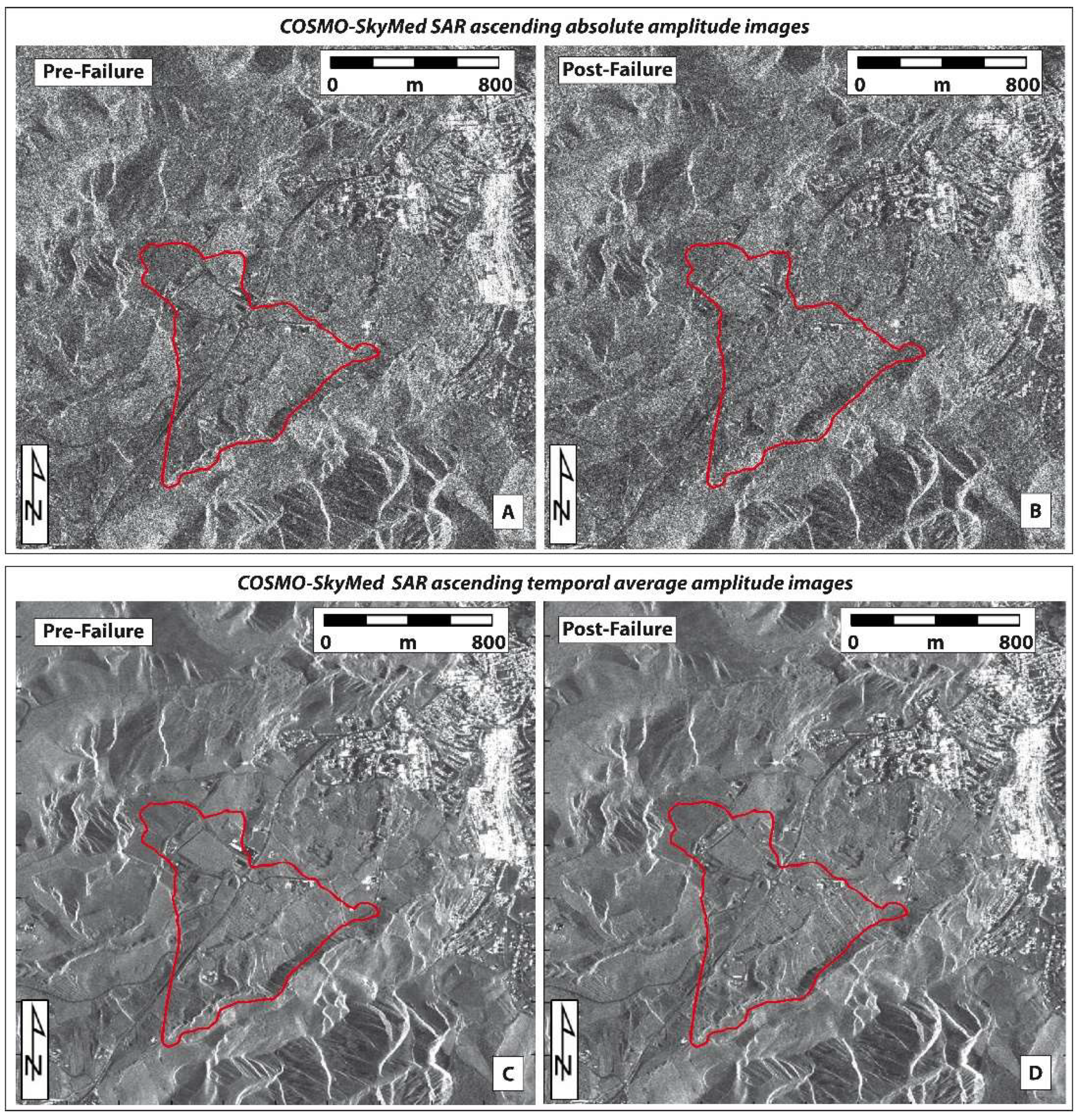
Figure 1. Schematic diagram of the basic principle of DIC.
Ijgi 07 00372 g001
Figure 2. Typologies of the subset transformation order [52].
Ijgi 07 00372 g002
Figure 3. SW slope of Montescaglioso Village, which was affected by the landslide occurrence (3 December 2013). Local evidence of damage to primary infrastructure and private fields (A,B) obtained during the field survey in July 2016, and buildings (C), from Reference [39]. Coordinate system: WGS84 UTM33N.
Ijgi 07 00372 g003
Figure 4. Complete COSMO-SkyMed (CSK) Synthetic Aperture Radar (SAR) amplitude imagery dataset used in the analyses (in both ascending and descending geometries). The red line represents the landslide failure occurrence. In this diagram, all the available CSK scenes have been reported by highlighting the scenes used for the temporal average filtering process (in yellow and red) and those used directly in the DIC analyses without applying any type of temporal or spatial filter (in blue and green). The number of CSK SAR absolute amplitude images (in both acquisition geometries) is part of the whole CSK dataset, which covers a wider temporal window.
Ijgi 07 00372 g004
Figure 5. Pre- and post-failure CSK SAR amplitude datasets (in ascending geometry). The difference between the absolute amplitude (A,B) and the temporal average amplitude imagery (C,D) is clearly visible.
Ijgi 07 00372 g005
Figure 6. Regions of interest (ROIs) (orange polygons) used in approach #1 and located in the immediate surroundings of the landslide (red polygon).
Ijgi 07 00372 g006
Figure 7. Regions of interest (ROIs) used in approach #2. Here, the ROIs have been intentionally designed over a wider sector by arbitrarily choosing those areas not affected by the general movement of the slope failure. In (A,B), two different series of ROIs have been highlighted in green tones (A) and red tones (B).
Ijgi 07 00372 g007
Figure 8. DIC displacement maps retrieved from CSK SAR ascending absolute amplitude images. Here, an increase in the areas affected by the decorrelated signal from (A) to (D) (highlighted in yellow polygons) in the surrounding sectors of the Montescaglioso landslide area (red polygons) is clearly visible. The time span between the pre-event (3 December 2013) and post-event images increases from the top left to bottom right: (A) 18 December 2013 (15 days); (B) 3 January 2014 (31 days); (C) 4 February 2014 (63 days); and (D) 8 March 2014 (95 days).
Ijgi 07 00372 g008
Figure 9. Temporal resolution effect on the decorrelation signal. A direct relationship was achieved, which is also perceptible from the trend line (dashed black line).
Ijgi 07 00372 g009
Figure 10. DIC displacement maps derived from CSK SAR absolute amplitude images (in ascending geometry) and analyzed with COSI-Corr software. The extracted vector field (white arrows) of the landslide area (red polygon) is reported. Grey coloring corresponds to areas with loss of correspondence between the pre- and post-failure images.
Ijgi 07 00372 g010
Figure 11. DIC displacement map retrieved from ascending CSK SAR temporal average amplitude images with COSI-Corr (A) and GOM Correlate (B) software. The white arrows show the displacement vector field. The red polygons show the landslide boundary. The stable area surrounding the slope failure area is clearly characterized as having no movement. Grey coloring corresponds to areas with loss of correspondence between the pre- and post-failure images. Therefore, the displacement magnitude effect induced an important or total variation on the morphology.
Ijgi 07 00372 g011
Figure 12. DIC displacement map retrieved from descending CSK SAR temporal average amplitude images with COSI-Corr software. The white arrows show the displacement vector field. The red polygons show the landslide boundary. Grey coloring corresponds to areas with loss of correspondence between the pre- and post-failure images.
Ijgi 07 00372 g012
Figure 13. DIC displacement map retrieved from LANDSAT 8 OLI-TIRS (Operational Land Imager-Thermal Infrared Sensor) images and analyzed with COSI-Corr software. White arrows show the displacement vector field. The red polygon shows the landslide boundary. Grey coloring corresponds to areas with loss of correspondence between the pre- and post-failure images.
Ijgi 07 00372 g013
Figure 14. DIC displacement map retrieved from shaded Digital Terrain Models (DTMs) derived images with COSI-Corr (A) and GOM Correlate (B) software. The white arrows show the displacement vector field. The red polygons show the landslide boundary. Grey coloring corresponds to areas with loss of correspondence between the pre- and post-failure images.
Ijgi 07 00372 g014
Figure 15. DIC displacement map retrieved from the HR (high-resolution) optical orthophoto with COSI-Corr software. The white arrows represent the displacement vector field direction of the landslide (red polygon), which is consistent with the other displacement maps. Grey coloring corresponds to areas with loss of correspondence between the pre- and post-failure.
Ijgi 07 00372 g015
Figure 16. Comparison between DIC analyses retrieved from the DTM dataset using COSI-Corr and GOM Correlate software.
Ijgi 07 00372 g016
Figure 17. Diagram showing the background noise (in pixels) histograms for each dataset considered using COSI-Corr software. Each curve represents the percentage of pixels (on the y-axis) characterized by different values of background noise/displacement accuracy (on the x-axis) for each dataset. For each curve, the most likely value of displacement accuracy (i.e., the one with the highest percentage of pixels) and the reliability interval above 30% of the measured background noise are shown.
Ijgi 07 00372 g017
Figure 18. Diagram showing the background noise (in meters) histograms for each dataset considered using COSI-Corr software. Each curve represents the percentage of pixels (on the y-axis) characterized by different values of background noise/displacement accuracy (on the x-axis) for each dataset. For each curve, the most likely value of the displacement accuracy (i.e., the one with the highest percentage of pixels) and the reliability interval above 30% of the measured background noise are shown.
Ijgi 07 00372 g018
Table 1. Detailed scheme of the technical specifications of the different analyzed datasets.
DatasetPlatformSensorImageGeometrical Resolution (m/pixel)Pre-Failure ImagePost-Failure Image
COSMO-SkyMed (CSK) ASCSatelliteSARSAR absolute amplitude 33 December 201318 December 2013
COSMO-SkyMed (CSK) DESCSatelliteSARSAR absolute amplitude 331 March 201320 December 2013
COSMO-SkyMed (CSK) ASCSatelliteSARSAR temporal average amplitude 319 May 2011–3 December 201318 December 2013–14 May 2015
COSMO-SkyMed (CSK) DESCSatelliteSARSAR temporal average amplitude 327 August 2009–31 March 201320 December 2013–24 May 2015
LANDSAT 8 OLI-TIRSSatelliteMulti-spectralPanchromatic1526 October 201315 February 2014
Digital Terrain Model (DTM)AirborneLiDARShaded relief1July 2013December 2013
OrthophotoAirborneOpticalHigh resolution<1July 2013December 2013
Table 2. Background noise retrieved by the region of interest (ROI) method: Approaches #1 and #2.
DatasetSensorImageApproach #1: Background Noise–MeanApproach #2: Background Noise–MeanΔ (Approach #1–Approach #2)
PixelPixelPixel
COSMO-SkyMed (CSK) ASCSARSAR absolute amplitude ~0.14~0.470.33
COSMO-SkyMed (CSK) DESCSARSAR absolute amplitude ~0.12~0.350.23
COSMO-SkyMed (CSK) ASCSARSAR temporal average amplitude ~0.12~0.100.02
COSMO-SkyMed (CSK) DESCSARSAR temporal average amplitude ~0.15~0.050.1
LANDSAT 8 OLI-TIRSMulti- spectralPanchromatic~0.10~0.050.05
Digital Terrain Model (DTM)LiDARShaded relief~0.81~0.800.01
OrthophotoOpticalOptical high-resolution~0.21~0.200.01
Table 3. Pixel percentage affected by the decorrelated signal increases as the time span between the processed images increases.
Master Image: 3 December 2013
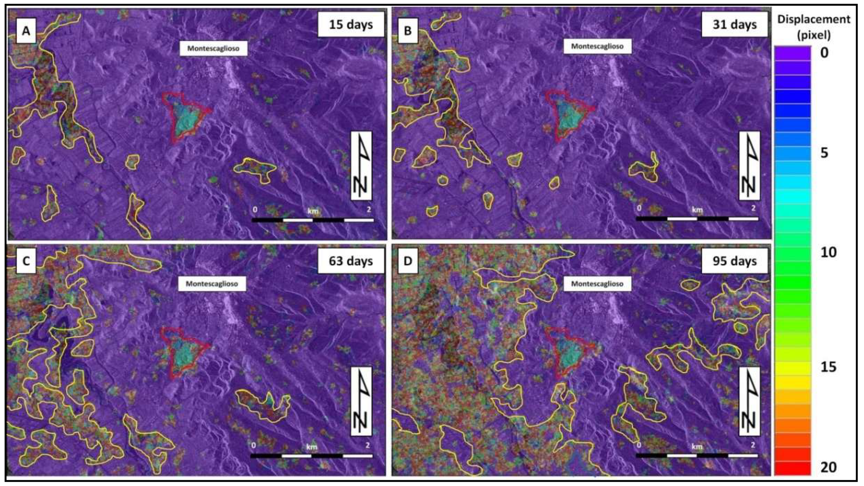
Post-Failure Images (Slaves)Time Span from Master Image (gg)Time Span from Master Image (years)Pixels Affected by Decorrelated Signal (%)
18 December 2013 150.0432.0
23 December 2013 230.0644.8
3 January 2014 310.0830.2
4 February 2014 630.1742.2
20 February 2014 790.2241.1
8 March 2014 950.2641.3
9 April 2014 1470.4043.6
25 April 2014 1630.4545.5
11 May 2014 1790.4945.9
12 June 2014 2110.5844.8
28 June 2014 2270.6246.6
Table 4. DIC setting parameters used in COSI-Corr and GOM Correlate processing.
DatasetCOSI-CorrGOM Correlate
Frequency Correlator EngineSurface ComponentPattern Quality ToolScale Calibration
Window Size (pixels)Step (pixels)Window Size (pixels)Point Distance (pixels)Window Size (pixels)Point Distance (pixels)
CSK SAR absolute ASC1284205205Manually defined scale
CSK SAR absolute DESC2568505505Manually defined scale
CSK SAR temporal average ASC642205205Manually defined scale
CSK SAR temporal average DESC1284505505Manually defined scale
LANDSAT 8 OLI-TIRS162505505Manually defined scale
Shaded DTMs644505155Manually defined scale
HR Optical Orthophoto1288505155Manually defined scale
Table 5. Analysis of equivalent points (IDs from 1 to 10) using COSI-Corr and GOM Correlate software showed consistent actual displacement values with only a slight error fraction.
IDDisplacement (pixel)
COSI-CorrGOM CorrelateΔ (COSI-Corr vs. GOM Correlate)
10.880.750.13
23.353.160.19
33.213.090.12
411.8911.350.54
512.6112.680.07
616.0716.260.19
718.3418.530.18
818.8919.070.18
916.3916.230.16
100.730.620.11
Table 6. Results achieved by the COSI-Corr and GOM Correlate software for the different datasets processed.
DatasetCOSI-CorrGOM Correlate
CSK SAR absolute ASCYesNo
CSK SAR absolute DESCYesNo
CSK SAR temporal average ASCYesYes
CSK SAR temporal average DESCYesYes
LANDSAT 8 OLI-TIRSYesNo
Shaded DTMsYesYes
HR Optical OrthophotoYesNo

