Nesting Patterns of Loggerhead Sea Turtles (Caretta caretta): Development of a Multiple Regression Model Tested in North Carolina, USA

Abstract

Numerous environmental conditions may influence when a female Loggerhead sea turtle (Caretta caretta) selects a nesting site. Limited research has used Geographic Information Systems (GIS) and statistical analysis to study sea turtle spatial patterns and temporal trends. Therefore, the goals of this research were to identify areas that were most prevalent for nesting and to test social and environmental variables to create a nesting suitability predictive model. Data were analyzed at all barrier island beaches in North Carolina, USA (515 km) and several variables were statistically significant: distance to hardened structures, beach nourishment, house density, distance to inlets, and beach elevation, slope, and width. Interestingly, variables that were not significant were population density, proximity to the Gulf Stream, and beach aspect. Several statistical techniques were tested and Negative Binomial Distribution produced good regional results while Geographically Weighted Regression models successfully predicted the number of nests with an average of 75% of the variance explained. Therefore, the combination of traditional and spatial statistics provided insightful predictive modeling results that may be incorporated into management strategies and may have important implications for the designation of critical Loggerhead nesting habitats.

1. Introduction

Multiple environmental cues may be important to the female sea turtle when deciding where to nest, and a combination of cues may help to explain more variation in the nesting patterns, than single environmental variables [1,2]. Loggerhead nests are typically found between the mean high water line and the toe of the dune or line of permanent vegetation and, in North Carolina, Loggerheads nest from late May to mid-August [3]. Females nest at intervals of every two to four years (not every year), typically laying three to six clutches per season, approximately twelve to fourteen days apart [4]. In nesting, females follow a series of steps: 1) emerge from the ocean, 2) select a nesting site by digging a body pit, 3) dig an egg chamber within the body pit, 4) deposit eggs inside of the egg chamber, 5) cover the eggs using rear flippers, 6) camouflage the nesting site, and 7) make a return crawl to the ocean [3]. Hatchling Loggerheads leaving the North Carolina coast migrate east to the Gulf Stream current before becoming entrained in the North Atlantic Gyre flowing around the Sargasso Sea. Most Loggerheads will remain within the gyre for several years, crossing to the eastern side of the Atlantic Ocean before returning as large juveniles to the North American coast to take up residence in coastal feeding grounds [4].

Suggestions have been made that, because oviparous species have short-term control over the timing of oviposition, the females may wait until the nesting conditions are optimal to minimize harm to themselves from predation or desiccation, while also maximizing the survival of their offspring [1]. 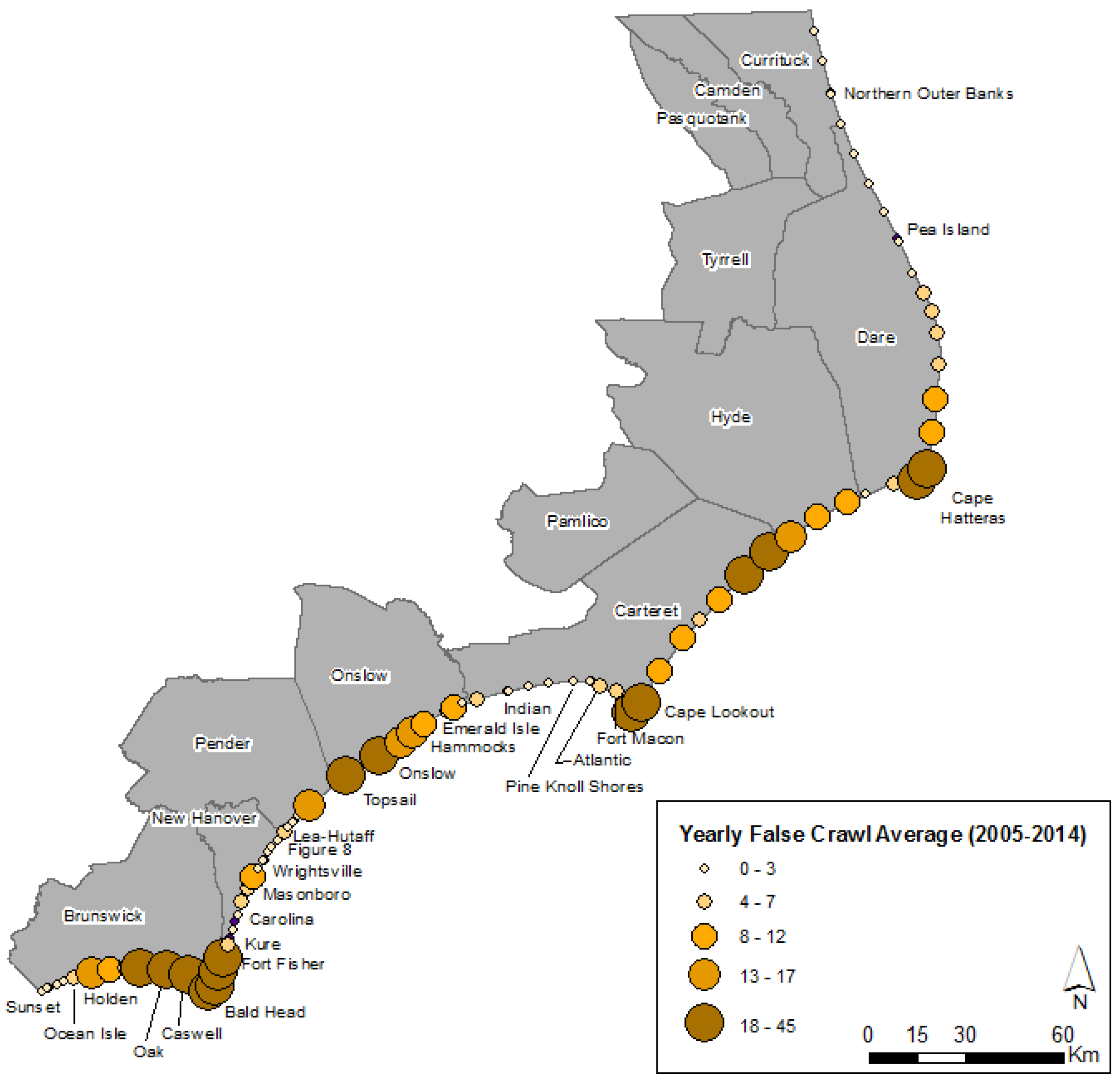Nest placement close to the sea increases the likelihood of inundation and egg loss due to erosion, whereas nest placement farther inland increases the likelihood of hatchling disorientation, desiccation, and predation of both eggs and hatchlings [5]. If a nesting female is uncomfortable with the potential nesting site, she will cross the beach without digging and return to the water. This act is termed a “false crawl” and could suggest that the environmental needs were not met or that she felt threatened by a predator or human activity [6]. Analyzing both nesting and false crawls is important when evaluating the correlations between environmental variables and nesting and false crawl densities.

1.1. Critical Loggerhead Nesting Habitat in North Carolina, USA

In December 2011, under the Endangered Species Act, the National Marine Fisheries Service and the U.S. Fish and Wildlife Service designated nine Distinct Population Segments (DPS) for Loggerhead sea turtles (Caretta caretta) [7]. Each DPS is labeled as either threatened or endangered. In North Carolina, Loggerhead sea turtles are a part of the Northwest Atlantic DPS and are designated as threatened. Effective August 2014, the USFWS designated specific areas in the terrestrial environment of the U.S. 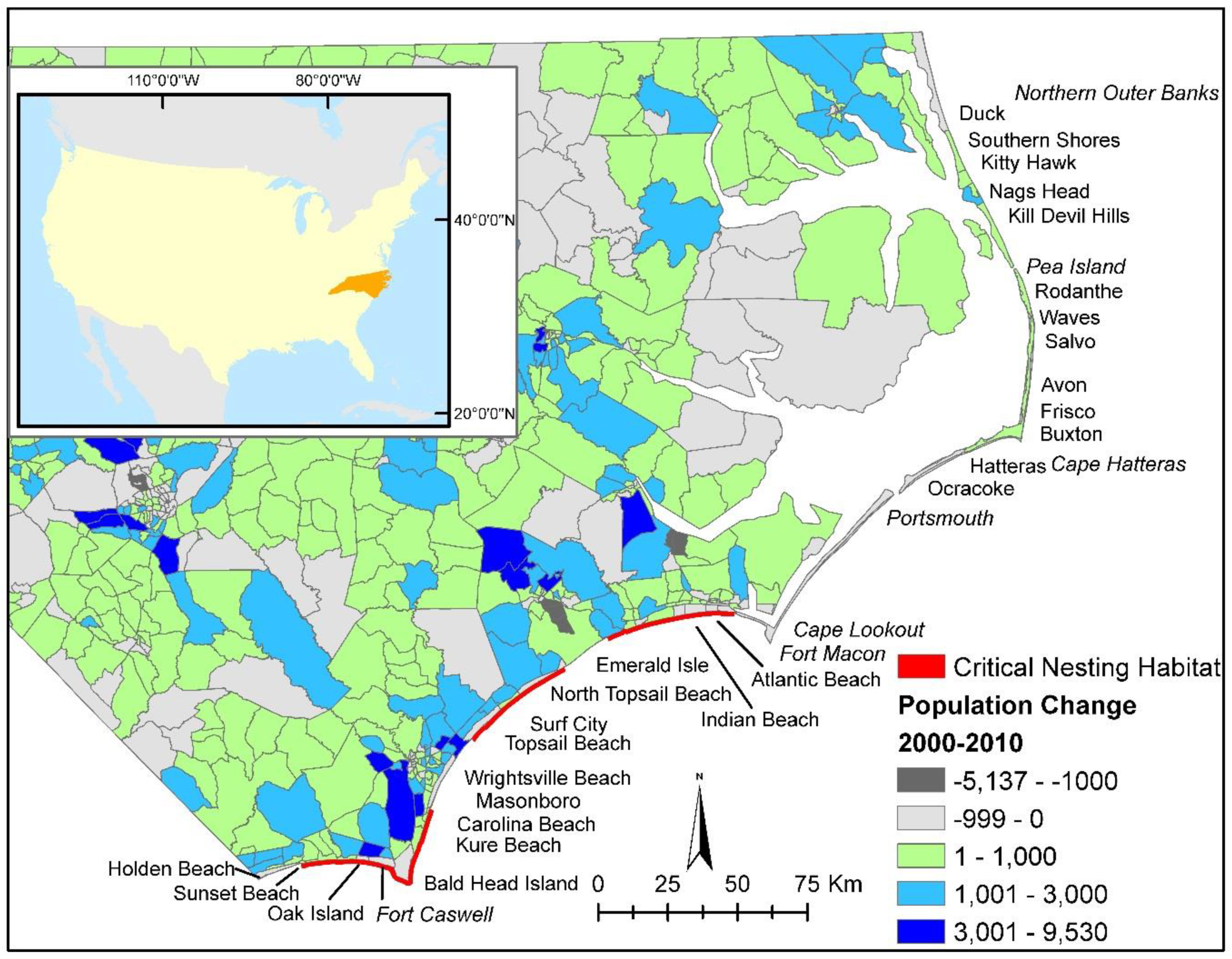Atlantic and Gulf of Mexico coasts as critical habitats for the Northwest Atlantic DPS [8]. In total, approximately 1102 km of shoreline are within the boundaries of the critical habitat designation. North Carolina, a member of the Northern Recovery Unit, has approximately 154.6 km as Critical Nesting Habitat. This designation includes popular tourism beaches such as: Atlantic Beach, Emerald Isle, Topsail Island, Carolina Beach, Kure Beach, Bald Head Island, Oak Island, and Holden Beach. Critical habitat designations were determined by examining nesting data from 2002–2012 and beaches with the highest nesting densities were selected. In addition, adjacent beaches were included in order to serve as expansion areas if the nesting rates changed. At this time, no management plans have been implemented to address Loggerhead sea turtles in any of North Carolina’s critical habitats [8].

1.2. Factors that Influence Nesting

Marine turtles experience threats from both natural and human sources [1]. It is estimated that only one of every 1000 eggs develops into an adult [9]. Natural threats coupled with additional stress placed on turtles from human activities have led to a need for increased research regarding possible management strategies.

1.2.1. Environmental Influences

Several studies have investigated correlations between nest site selection and topographic variables; however, there are some inconsistencies among the findings. Beach width has been identified as the primary factor affecting nest site selection and that wider beaches (>8.5 m) had more nests than narrow beaches [10]. Beach width has been negatively correlated with beach slope, indicating that wider beaches have inherently less slope. Interestingly, others have concluded that beaches with steeper slopes and higher elevation had higher nest densities. Steeper slopes indicate areas with higher elevation and thus have a higher probability of nest survival [5,11].

1.2.2. Human Influences

When development in the coastal zone increases, the pressures that threaten biodiversity can increase as well. Urbanization of beaches has led to the increased construction of houses, which in turn contributes to the increased amount of artificial light. Research has investigated the responses of sea turtles to artificial light [3]. Sea turtles were presented with different types of luminaries and found that light significantly reduced the number of Loggerheads emerging and nesting in the lighted study areas. Some turtles were also misdirected on their return to the ocean after nesting attempts. More recently, research concluded that nesting densities are negatively related to night light intensity and that nests are concentrated in darker areas along the coast [12]. A study conducted in 1995 demonstrated a positive correlation between nesting densities and the presence of tall objects, such as buildings or dunes [13]. This response may be unique to urban beaches to avoid being exposed to light. Artificial light also affects hatchlings emerging on urban beaches where they do not orient towards the ocean [14].

Development adjacent or near to the coastal zone has also led to an increase in erosion in some areas, which has resulted in beach nourishment and coastal armoring (e.g., jetties, groins, rock walls, and sandbags). Research has been conducted to investigate the influence that hardened structures may have on sea turtle nesting and although it is hypothesized that barriers impact nesting, it has also been shown to not have an effect on the nesting rate [3]. Extensive studies have been carried out to investigate the effects of beach nourishment and sediment characteristics on nesting and hatching success. An issue with beach nourishment is the unintentional creation of escarpments. Research in Florida has shown that slope, volume, and beach profile may be the most important environmental cues for sea turtle nesting [15]. At the start of a nourishment project, the U.S. Army Corps of Engineers (USACE) constructs a berm that extends the shoreline profile seaward. The berm is constructed in such a way that over time it will gradually return to the original profile, creating somewhat of a lag time from when the profile is constructed and when it will return to a state of equilibrium [16]. If the berm construction is done close to the nesting season, it may deter some females from nesting. Additionally, it may take a year or more for a nourished beach to return to its original profile and an increased number of false crawls in these areas can be seen for up to two years [16]. Additional concerns of nourishment on sea turtles include the quality and characteristics of sand placed on the beach. In 2007, the North Carolina Division of Coastal Management implemented a list of sediment criteria rules [17]. The focus of these rules was mostly ensuring that the sediment size of the dredged sand matches that of the native sand. Sand that contains too much silt or fine shell material can become compacted, making it too difficult for females to dig their egg chambers [18].

The color of dredged sand is not considered in the current list of criteria; however, nourished sand is typically darker than the native sand found on these beaches. Sea turtles exhibit temperature dependent sex determination, meaning that the surrounding temperature determines their sex during the middle third of the incubation period. Warmer beaches with darker sand will produce more females, while cooler lighter beaches will produce more males [19]. North Carolina is the northern nesting limit for the Northwest Atlantic Ocean Loggerhead Sea Turtle distinct population segment and beaches have relatively cooler sand compared to beaches located further south such as Florida and Georgia. North Carolina beaches produce 42% male hatchlings, while Florida only produces about 10% [20].

1.3. Project Significance and Objectives

Very little work has been done to merge the study of sea turtle conservation with Geographic Information Systems (GIS) as a way to view data from both a statistical and geographical standpoint. Although similar studies have identified environmental variables that are statistically significant to nest site selection of Loggerhead sea turtles, very few studies have used a combination of multiple variables over a large geographic area. Most studies are restricted spatially to the local level, where one beach was studied. Therefore, the primary research objective was to develop a predictive geographic model that covers a large area and statistically compares multiple human and environmental variables. The variables tested included: elevation, slope, aspect (cardinal direction), beach width, distance to hardened structures (e.g., pier or jetty), distance from inlets, housing density, population density, proximity to the Gulf Stream, and location of beach nourishment. Understanding the environmental and social conditions that affect nesting patterns will give insight into how the females might react to potential global changes (e.g., sea-level rise) and resulting changes to beach morphology. The results from this project may have important implications for the designations of critical habitats and to the future management of Loggerhead rookeries. The following questions were investigated:

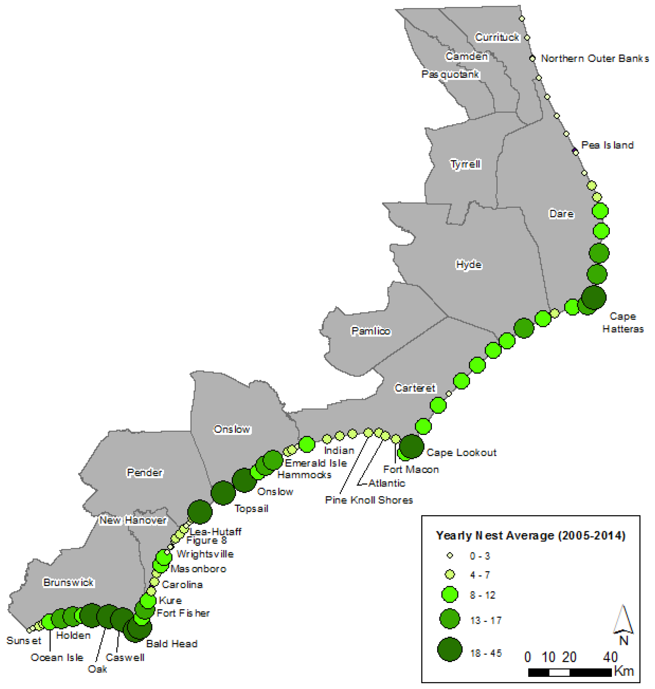
• Given that North Carolina is the northern extent for Loggerhead nesting, what areas of the North Carolina (NC) coast have the most and least nesting?
• Given the variety of studies that have identified several different variables of importance to sea turtle nesting, what environmental and human variables (alone and in combination) have the most statistically significant relationship with nesting locations in North Carolina?
• Given that there are currently no management plans for the designated Critical Nesting Habitats, which statistical technique is the most useful for explaining nesting distribution and can predictive modeling be used to identify how characteristics differ across large geographic areas?

1.4. Study Area

The North Carolina Sea Turtle Project, overseen by the North Carolina Wildlife Resource Commission’s Division of Wildlife Management, is a monitoring program that includes all beaches in North Carolina with the exception of Brown’s Island, a 4 km barrier island located north of Topsail Island, which is managed by the Camp LeJeune military base [21]. Each beach is surveyed during the nesting season by employees and volunteers from different organizations (see Appendix A for a detailed list of sea turtle nest monitoring programs in North Carolina). Nest characteristics are recorded and a GPS coordinate is obtained. At the end of each nesting season, all data are integrated into the project database.

To investigate the relationship between Loggerhead nesting and environmental and human variables, we studied all North Carolina beaches, approximately 515 km (Figure 1). The entire NC beach zone was selected for this study in order to investigate the variety of nesting densities and test the significance of environmental characteristics and human variables that may explain the density of sea turtle nests. Examining the entire North Carolina coastline allows for the evaluation of independent variables across a large geographic area which enables a thorough investigation of spatial variability. Additionally, population estimates indicate that there are approximately 865,000 people living along North Carolina’s coast and the barrier islands have seen a 75–150% population growth since 1980 [22].

To define the nesting area, heads-up digitizing was performed using both high-resolution Lidar data and orthophotography to create a line along the highest elevation of the dunes. This line represents the landward boundary for nesting. The official state shorelines, mapped by the North Carolina Department of Environment and Natural Resources, Division of Coastal Management, were gathered for all available years (2004, 2009 and 2012) [23]. The shoreline was defined as the boundary between wet and dry sand and with the digitized dune line this area became the potential nesting area for each island. Each of the beaches/islands were divided into transect polygons/zones. Transect polygons were created using the shoreline, dune line, and equal distances along the beach, but to determine the optimal number of transects for the 515 km of shoreline, a sensitivity analysis was conducted. The smallest transects, spaced 500 m, resulted in too many polygons with no nests, and polygons larger than 5000 m did not have enough polygons on each island in order to determine if parts of the island had different patterns of nesting through time. Therefore, the 5000 m transect polygons had enough zones (81) to identify spatial patterns across the 23 islands and not too many dates with 0 observations. Therefore, each island, was divided into approximately 5000 m length to create a total of 81 transect polygons, which were then used as the geographic unit of analysis. Next, to determine if there were regional trends across the study area, the 81 transects/23 islands, were grouped into 5 geographic regions: (1) northern Outer Banks, (2) Pea Island to Cape Hatteras, (3) Portsmouth to Cape Lookout, (4) Fort Macon to Bald Head Island, and (5) Fort Caswell to Sunset Beach.

2. Materials and Methods

To investigate the relationship between nesting locations and independent variables for each of the 23 islands, the project workflow consisted of: (1) data collection, preparation and processing, (2) statistical analysis, and (3) development of nesting suitability regression models.

Table 1. Data sources and purpose for model development.

Purpose	Model Variable(s)	Data Provider	Data Source/URL
Basemap Data	Critical Nesting Habitat	National Marine Fisheries Service, National Oceanic Atmospheric Administration (NOAA)	http://www.nmfs.noaa.gov/pr/species/turtles/criticalhabitat_Loggerhead.htm
	Shorelines, Beach Access Locations, Inlet Hazard Areas	North Carolina Department of Environmental Quality	https://deq.nc.gov/about/divisions/coastal-management/coastal-management-data/spatial-data-maps
	Primary Dune line	Digitized from NOAA Digital Coast Lidar data	https://coast.noaa.gov/dataviewer/#
Dependent variables	Nest and False Crawl Locations (2005 through 2014)	North Carolina Wildlife Resources Commission	Data provided by the organization
Environmental Independent Variables	Beach elevation, slope, aspect	NOAA Digital Coast Lidar data	https://coast.noaa.gov/dataviewer/#
	Beach width	Distance between dune line and shoreline	Calculated from dune line and shoreline
	Distance to Gulf Stream	NASA’s Physical Oceanography Distributed Active Archive Center	Night-time sea surface temperature (SST): https://podaac.jpl.nasa.gov/
	Distance to Inlets	NC OneMap	Digitized from 2012 orthophotography: http://data.nconemap.com/geoportal/catalog/main/home.page
Human independent variables	Population Change 2000–2010 (by Census Tract)	University of North Carolina: Carolina Population Center	http://demography.cpc.unc.edu/resources/nc-neighborhood-change-2000-2010/
	Population Density and Seasonal Housing (by Census Tract)	US Census Bureau	https://www.census.gov/geo/maps-data/data/tiger.html https://factfinder.census.gov/faces/nav/jsf/pages/index.xhtml
	Distance to Artificial Structures	North Carolina Department of Environmental Quality and NC OneMap	https://deq.nc.gov/about/divisions/coastal-management/coastal-management-data/spatial-data-maps and some digitized from 2012 orthophotography: http://data.nconemap.com/geoportal/catalog/main/home.page
	Density of oceanfront Houses	NC OneMap	Digitized from orthophotography: http://data.nconemap.com/geoportal/catalog/main/home.page
	Beach Nourishment	Western Carolina University Program for the Study of Developed Shorelines	https://psds.wcu.edu/current-research/beach-nourishment/

provides a list of data sources.

2.1. Data Collection, Preparation and Processing

2.1.1. Dependent Variables: Nesting and False Crawl Monitoring Data

Nesting and false crawl locations from surveys conducted annually from 2005 through 2014 were obtained from the North Carolina Wildlife Resources Commission. Data included: (1) geographic coordinates, (2) date collected, (3) species of turtle, and (4) activity type. Due to inaccuracies in GPS data collection, some nest and false crawl locations were plotting in impossible nesting locations, such as far inland or in the ocean, so these points were removed from the dataset. Sea turtle monitoring programs use GPS receivers to record the location of the nest and unfortunately, they do not have the funding to use mapping-grade GPS receivers. Also, there is no documentation for the mapping methods, or standards, for field mapping (e.g., how long they wait before taking a waypoint, number of satellites, and the minimum spatial resolution) and post-processing (e.g., differential correction). The point locations can range from 3–5 m, if the greatest care was taken during collection, to 20–30 m if data were less accurately collected and had no post-processing. Therefore, on average, the nesting data were estimated to be 20 m accurate. Points were also removed from further analysis if they were a species of sea turtle other than Loggerhead (Caretta caretta). By far the Loggerhead turtle is the most prevalent species nesting in North Carolina and other species are not as common and do not have the numbers to enable developing a species distribution model.

Nests deposited in areas with low probability of success are often times relocated to areas with a higher probability of success. Relocation sites were not included in data analysis because the new location is the only recorded coordinate and these locations will not help the development of a nest prediction model. It is important to note that nesting and false crawl data were incomplete for some dates and these were coded appropriately, as missing values, so as not to interfere, or incorrectly influence, the statistical analysis techniques.

2.1.2. Environmental Variables: Beach Elevation, Slope. Aspect and Width

Lidar data were the primary data source used to derive beach elevation, slope and aspect. Lidar uses a pulsed laser to measure variable distances to the Earth. The light pulses, combined with additional data recorded by the airborne system, generate precise three-dimensional information about the shape of the Earth and characteristics of the surface. Lidar data are of particular interest to researchers in coastal areas because of the ability to quickly highlight small elevation differences across the coastal landscape and have successfully been used when other commonly used digital elevation models were not adequate due to the temporal or spatial resolution [26].

Lidar data were obtained from the National Oceanic Atmospheric Administration (NOAA) Digital Coast “Coastal Lidar Data Registry” for all available years between 2005 and 2014 (in the WGS84 geographic coordinate system, NAD83 horizontal datum and NAVD88 vertical datum) [27]. The data were from multiple mapping projects carried out by the US Army Corp of Engineers, National Coastal Mapping Program, the Joint Airborne Lidar Bathymetry Technical Center of Expertise, the National Geodetic Survey Remote Sensing Division, and the United States Geological Survey Coastal Marine Geology Program (

Table 2. Lidar data sources and accuracies.

Year	Collection Dates	Source	Horizontal Accuracy	Vertical Accuracy
2005	24 August–26 November	USACE National Coastal Mapping Program	+/− 3.0 m within two standard deviations	+/− 3.0 m within two standard deviations
2008	17 March–27 March	NOAA National Geodetic Survey Remote Sensing Division	+/− 3.0 m within two standard deviations	+/− 3.0 m within two standard deviations
2009	16 August–24 August	USACE Joint Airborne LiDAR Bathymetry Technical Center of Expertise	+/− 0.75 m within one standard deviation	+/− 0.20 m within one standard deviation
2009	27 November–1 December	USGS Coastal Marine Geology Program	+/− 3.0 m within two standard deviations	+/− 3.0 m within two standard deviations
2010	4 May–16 June	USACE Joint Airborne LiDAR Bathymetry Technical Center of Expertise	+/− 0.75 m within one standard deviation	+/− 0.15 m within one standard deviation
2011	28 August–29 August	NOAA National Geodetic Survey Remote Sensing Division	+/− 1 m within two standard deviation	+/− 0.30 m within one standard deviation
2012	8 November–29 November	USGS Coastal Marine Geology Program	+/− 0.194 m within one standard deviation	+/− 0.147 m within one standard deviation
2013	23 May–14 June	USACE Joint Airborne LiDAR Bathymetry Technical Center of Expertise	+/− 0.75 m within one standard deviation	+/− 0.15 m within one standard deviation

). Using ArcGIS, the first return Lidar grids were clipped to the study area, projected to the North Carolina State Plane coordinate system (FIPS 3200 and units in meters) with a cell size of two meters by two meters, and mosaicked together using mean as the mosaic operator. The 2 m cell size was chosen as the average resolution of the data sources and resulted in a consistent grid for each year of data. For 2009, when there were two dates of Lidar data, the average elevation was calculated.

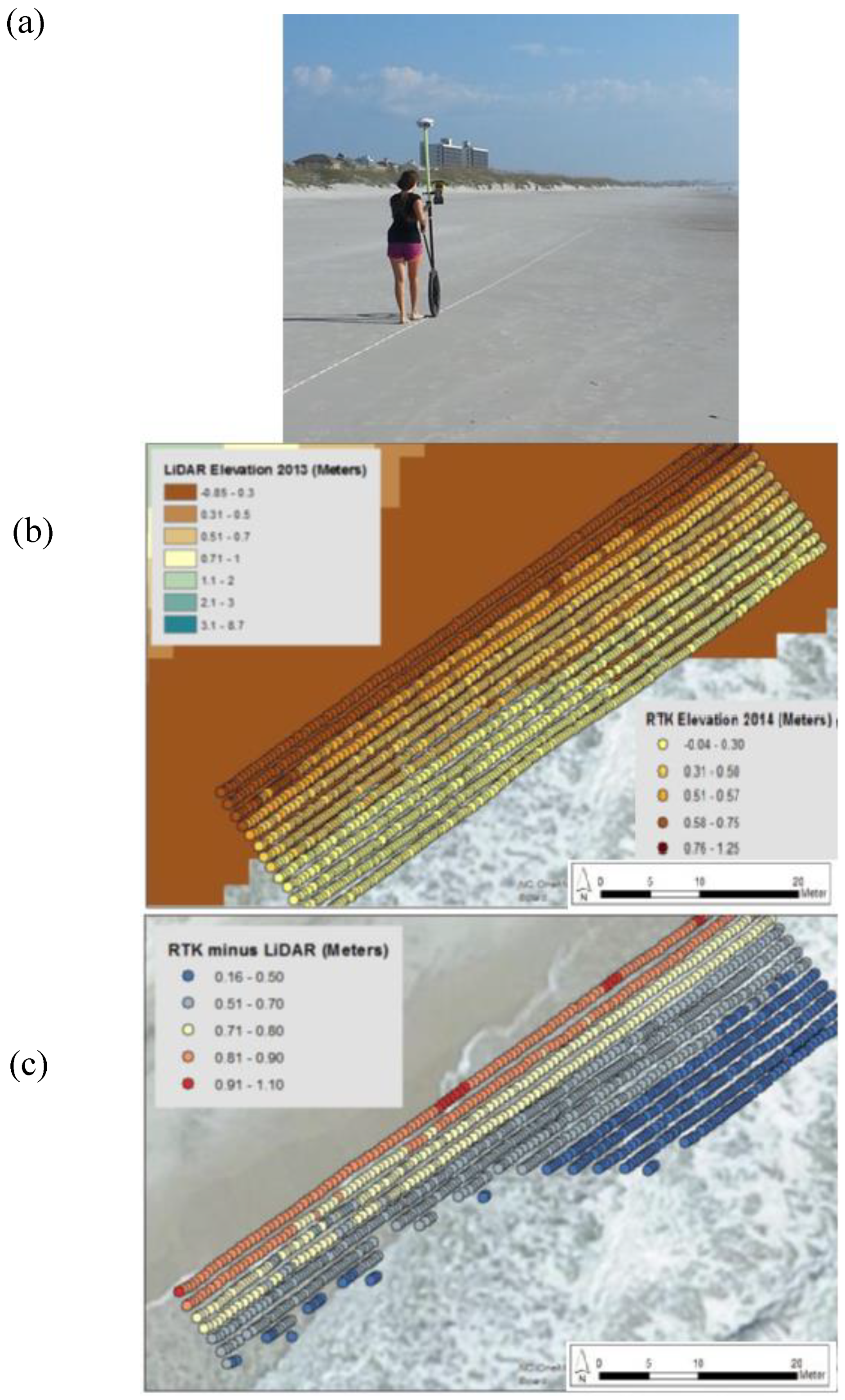
Beaches in North Carolina are dynamic and can change both seasonally and from storm events [28,29,30,31]. Field work was conducted to collect elevation data to be compared with the Lidar data to test the validity of Lidar for beach morphology metrics. Eight sites were selected based on a variety of nesting density, infrastructure and population/housing density along the beach. Fieldwork was conducted at Topsail Beach, Wrightsville Beach, Masonboro Island, and Bald Head Island (Figure 1).

Near-shore elevation data were collected using a survey grade Trimble Real Time Kinematic (RTK) unit. Data were collected at low-tide to ensure that the greatest amount of the near-shore environment was captured. With the GPS receiver mounted on a rover rod, data were collected by recording X,Y,Z data every 0.5 m in parallel lines to the water’s edge and then repeated at 1 m intervals towards the dune line. Elevation data were collected in North America Vertical Datum 1988, consistent with the Lidar data. The field data were compared with the Lidar data to evaluate the accuracy of the Lidar. If the field data and Lidar data are comparable then the assumption is that the rest of the Lidar data accurately represents the study area and can be used for further analysis. It is important to note that temporal differences exist as the Lidar data were collected in June 2013 and the RTK field elevation data were collected in May 2014. Inherently, some variation in elevation data may exist as the near-shore environment is dynamic and beach nourishment did occur at some of the field sites between 2013 and 2014. However, the seasonal influence is accounted for in that the Lidar and field work were collected at the same time of year. A comparison of the RTK and Lidar data showed that over 90 percent of the data points were less than 1 m difference in elevation. Therefore, the RTK and Lidar data were comparable which validated the use of Lidar to derive several beach metrics used in the study (Figure 2).

Using ArcGIS spatial analysis tools, slope grids were generated from the Lidar Digital Elevation Model (DEM) grids by calculating the rate of change in z-value from each cell of the raster surface and was recorded in degrees. Aspect grids were generated by identifying the linear directional mean and circular variance using several dates of shorelines (2004, 2009, and 2012). Lastly, for each transect polygon, the average elevation, slope and aspect were calculated for each year.

Beach width was calculated by measuring the distance (in meters) from each vertex of the dune line (described above in Section 1.4) to the nearest shoreline, for each of the three years that a shoreline was available. For each transect polygon and year, an average beach width was calculated.

2.1.3. Environmental Variables: Distance to Gulf Stream and Inlets

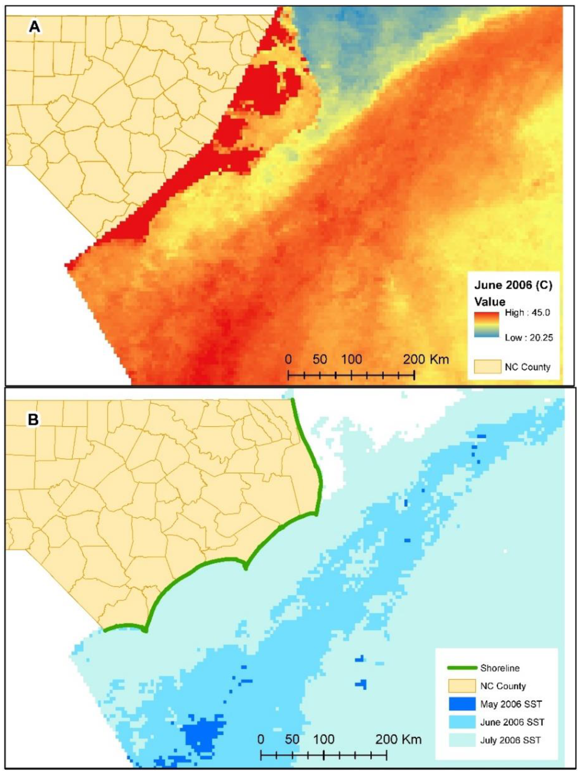
To derive the location of the Gulf Stream, night-time sea surface temperature (SST) data were obtained from NASA’s Physical Oceanography Distributed Active Archive Center as level 3 monthly and 8-day composite images [32]. Monthly data were from the MODIS (Moderate Resolution Imaging Spectroradiometer) Terra, Level 3, Thermal Infrared (4-km cell size) sensor from June, July and August, for the years 2005 through 2014. The eight-day images were also from the MODIS Aqua, Level 3 Thermal Infrared (4-km cell size) sensor and were used for the last eight days of May, for the same years. The composite night-time SST images were derived from the 11 and 12 micrometer thermal infrared bands (MODIS channels 31 and 32).

Data were converted to ArcGIS grids using the Marine Geospatial Ecology Tools from Duke University’s Marine Geospatial Ecology Lab [33]. Loggerhead sea turtles are most widely sighted in waters with an average SST of 26–29 °C during the warm nesting months (May–August) [34]. Therefore, SST grids were analyzed for each month of the nesting season, and all years of the study (2005–2014) in order to reflect the location of the Gulf Stream current in the North Atlantic. A query extracted the areas with the desired temperature range and polygons were created for each month (May, June, July, and August) and each year (2005–2014) (Figure 3). The distance from each transect polygon to the nearest monthly and annual SST polygon was calculated and then the yearly average distance was calculated for each transect polygon.

Distance to the nearest inlet was determined by first digitizing points in the middle of each of the 21 inlets and then measuring the distance from each nest to the nearest inlet. For each transect polygon, the average yearly distance to inlets was calculated.

2.1.4. Human/Social Variables: Population Change, Density and Seasonal Housing

Population change (2000–2010) data were obtained from the Carolina Population Center [24]. In order to aggregate these Census Tract data to the transect polygons, the data were interpolated using the Inverse Distance Weighted (IDW) method and then an average per transect polygon was calculated. Total population data were obtained from the 2000 and 2010 Census of Population also at the Census Tract level of geography [35]. These data were interpolated using IDW to calculate population density (people per hectare) and then averaged for each transect polygon.

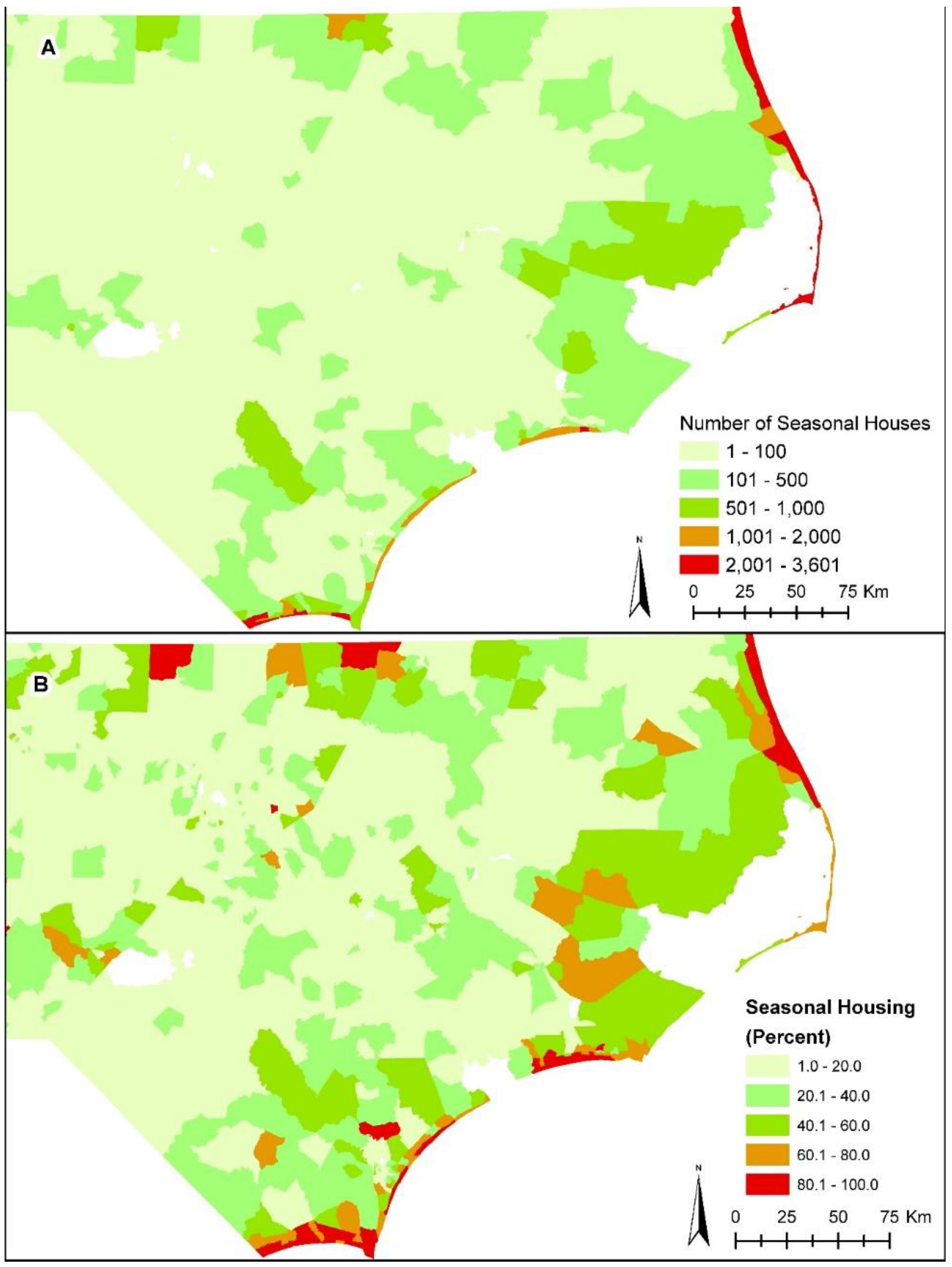
Tourism is a primary component of the coastal economy and understanding the seasonality of the population during the summer months may have an influence on the human impact more so than the total population of permanent residents. Therefore, the total number of housing units and the number of seasonal units (by Census Tract) were used to calculate the percent change in seasonal housing from 2000 to 2010 (Figure 4). These data were also interpolated using IDW and an average per transect polygon was calculated.

2.1.5. Human/Social Variables: Artificial Structures

Artificial structures include piers, jetties, groins, rock walls, sand bags, and boardwalks. Data were obtained from the North Carolina Department of Environmental Quality, Division of Coastal Management, which used 2007 rectified orthophotography to digitize the location of shoreline structures at a scale between 1:300 and 1:500 feet [36]. To ensure that we had a complete dataset, 2012 orthophotography was checked and any missing, or recently constructed structures, were digitized. The total number of structures per transect polygon was calculated. Also, the distance between each sea turtle nest to the nearest structure was calculated and then the average distance per transect was computed for each year.

2.1.6. Human/Social Variables: Oceanfront Houses

The number of houses located along the shoreline can be considered as potential sources of artificial light and human disturbance or influence on the coast. Therefore, oceanfront houses were digitized using 2012 orthophotography [37]. Housing density was calculated as the number of houses per hectare and averaged for each transect polygon. Only 1 date (2012) of orthophotography was available for the entire study area and therefore this housing count and density were used for each year in the study.

2.1.7. Human/Social Variables: Beach Nourishment

Information regarding the completion of beach nourishment projects was obtained from The Program for the Study of Developed Shorelines at Western Carolina University [38]. Projects labelled as shoreline protection or emergency beach nourishment were included and the year of each project was recorded. All nourishment events for three years prior to the beginning of this study period (2003–2014) were also included in order to account for the gradual return of the berm to its natural state. The total number of nourishment projects was calculated for each transect polygon and each year.

2.2. Statistical Analyses

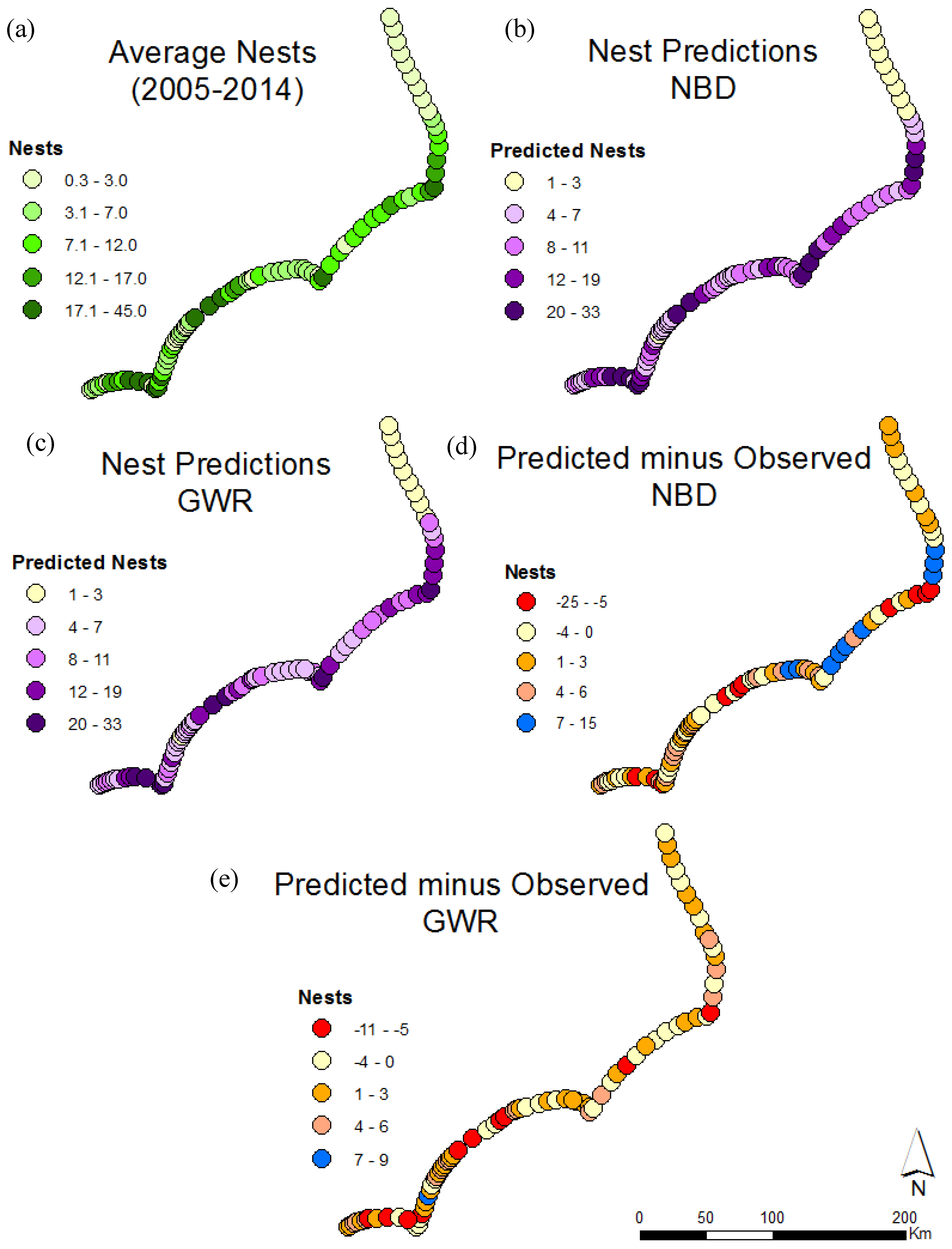
The objectives in a conservation study such as this are to evaluate the correlations between nest densities (dependent variable) and one or more independent environmental and human variables. To identify which independent variables were significantly correlated with annual nesting observations, a Generalized Linear Model (GLM) was run using Statistical Analysis System (SAS). GLM’s provide a powerful tool for analyzing count data, such as the number of nests per transect polygon. The starting point for analyzing count data was to determine if the data meet the assumptions of a Poisson distribution by testing if the variance was greater than the mean, or if the number of zeros was greater than expected. The nesting count data used in this research did not fit the Poisson test, because the observed variance was higher than the variance of a theoretical model, suggesting that there was an over-dispersion of nesting data. 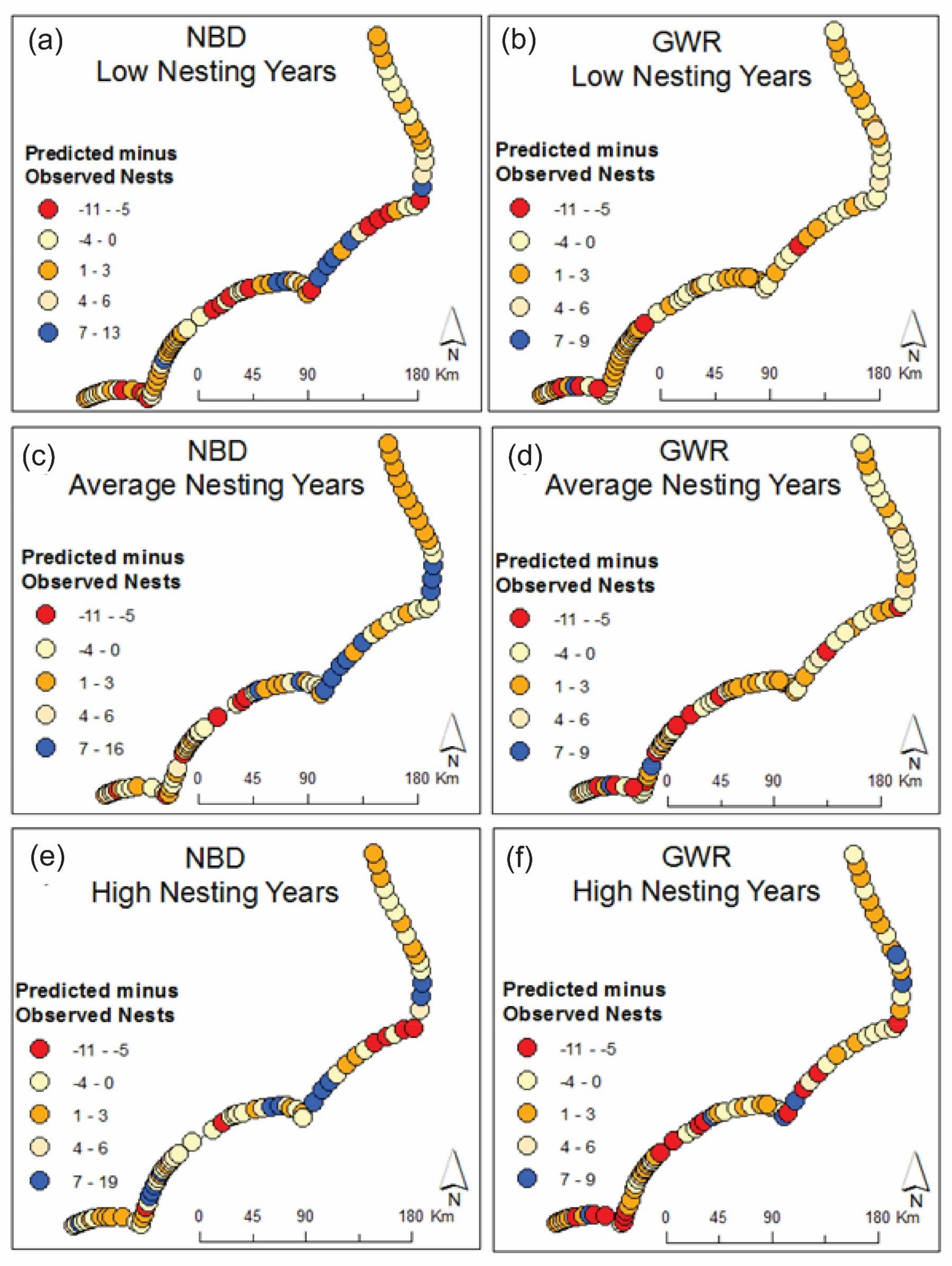Over-dispersion is to be expected, as nesting densities are heterogeneous (non-uniform) contrary to the assumptions implicit in widely used simple parametric models [39]. Both the dispersion parameters and goodness of fit test indicated that the Negative Binomial Distribution (NBD) technique was best suited for the nesting count data. Some of the independent variables were converted from ratio to categorical variables to provide another method of analyzing the data. For example, the distance to inlet variable was also included as distance categories: (1) 0 to 5000 m, (2) 5001 to 10,000 m and (3) > 10,000 m. The number of structures per transect polygon was also included as a categorical variable with 5 classes: (1) 0 structures , (2) 1–2 structures, (3) 3–5 structures, (4) 6–8 structures and (5) 9 or more structures.

First, an NBD model was created for the all years (2005 through 2014) which meant there were 10 years of nesting observations for each transect polygon which were compared with the independent variables. Importantly, some of the independent variables changed through time. For example, beach elevation, width and slop as well as SST and nourishment data were annual variables. The shoreline aspect (direction)variable, was based on the three dates of available shorelines (2004, 2009, and 2012) and all other variables were a single point in time or time period (e.g., Census data was from 2000 to 2010). Therefore, the NBD models compared data annually, not in total, in order to see if there were changes in relationships through time.

Building on the results from the NBD analysis, Geographically Weighted Regression (GWR) models were developed to provide local models by fitting a unique regression equation for each transect polygon. The GWR technique uses a moving weighted window (kernel or bandwidth) over the study area and computes a unique regression equation (with r-squared values, coefficients for each variable and goodness-of-fit measured using residuals) to each polygon. Spatial variation of the coefficients can be taken as an indication for non-stationarity [40]. Statistical non-stationarity exists when the properties of a time series dataset, such as mean, variance, and autocorrelation, are not constant over time.

Using the same dependent variable as the NBD analysis, the yearly number of nests per transect polygon was used as the dependent/response variable in the GWR analysis. Environmental and human variables that were significant in the NBD analysis were included in the GWR models as predictor variables. First, a spatial sensitivity test was performed where GWR models were calculated for a range of bandwidth sizes using kernal distance and number of neighbors. The values tested ranged from 2 to 5 number of neighbors and distanced from 10,000 m to 50,000 m in increments of 10,000 m. Results (r-square values and residuals) were compared with the standard method of using the AICc (corrected Akaike Information Criterion) [40]. GWR models were computed for each individual variable and combinations of variables.

3. Results

3.1. Distribution of Sea Turtle Nests and False Crawls

In total, 7009 Loggerhead nests and 5997 false crawls were located within the study area from 2005 through 2014. These data were summarized by transect polygon and year. Highest nesting densities were seen at Cape Lookout and Cape Hatteras, as well as Topsail Island and the southern region of the state (Oak Island, Caswell Beach and Bald Head Island) (Figure 5). High numbers of false crawls were in similar locations (Figure 6). Low nest and false crawl densities were in the northern Outer Banks, Wrightsville Beach, and Sunset Beach. Fluctuations in nest counts corresponded with the female nesting interval of two to four years [4]. Yearly nesting data were compared to the ten-year average to determine low (2007, 2009, 2014), average (2005, 2006, 2008), and high (2010–2013) nesting years.

The U.S. Fish and Wildlife Service considers a 1:1 false crawl to nest ratio as normal for an undeveloped beach. A higher ratio of false crawls to nests can indicate that the nesting environment is not favorable [9]. In this study, in North Carolina, developed beaches consistently had more false crawls than nests (

Table 3. Number of false crawls (FC), nests (N), yearly ratio of FC to N, and average FC to N ratio for each beach/island in North Carolina from 2005 to 2014.

Location (North to South)	Name	Number of Years Surveyed (FC/N)	Developed (D)/Undeveloped (U)	Average Yearly Number of False Crawls (FC)	Average Number of Nests (N)	Yearly Ratio (FC to N)	Aver-Age FC/N
1	N. Outer Banks	10/10	D	10.8	5.5	3.08	1.96
2	Pea Island	9/9	U	13.6	17.4	0.72	0.78
3	Cape Hatteras	6/7	U	129.3	158.0	0.79	0.82
4	Cape Lookout	5/5	U	156.2	163.6	0.96	0.95
5	Fort Macon	10/10	U	0.9	3.7	0.26	0.24
6	Atlantic	10/10	D	2.2	3.2	1.04	0.69
7	Pine Knoll Shores	9/9	D	3.0	5.9	0.41	0.51
8	Indian	10/10	D	0.9	3.4	0.31	0.26
9	Emerald	10/10	D	8.2	15.6	0.62	0.53
10	Hammocks	10/10	U	16.5	15.3	1.28	1.08
11	Onslow	9/9	U	40.1	44.4	0.93	0.90
12	Topsail	10/10	D	73.7	83.8	0.89	0.88
13	Lea-Hutaff	10/10	U	4.4	6.5	0.68	0.68
14	Figure Eight	9/9	D	8.7	12.9	0.73	0.67
15	Wrightsville	10/10	D	2.8	4.5	0.86	0.62
16	Masonboro	8/9	U	17.9	19.9	0.94	0.90
17	Carolina	10/10	D	3.9	6.4	0.75	0.61
18	Kure	9/9	D	5.3	7.6	1.02	0.71
19	Fort Fisher	10/10	U	30.8	25.9	1.15	1.19
20	Bald Head	10/10	D	86.4	66.2	1.33	1.31
21	Caswell	10/10	D	29.0	26.0	1.09	1.12
22	Oak Island	10/10	D	85.5	67.5	1.29	1.27
23	Holden	10/10	D	29.9	33.2	0.89	0.90
24	Ocean Isle	7/9	D	9.9	14.4	0.72	0.68
25	Sunset Beach	10/10	D	6.1	9.4	0.76	0.65

). Undeveloped beaches, such as Cape Hatteras National Seashore, generally had a higher number of nests than false crawls; however, there were some excpetions especially when an undeveloped beach was adjacent to a highly developed beach. This pattern suggests that undesirable nesting conditions (higher false crawl to nesting ratio) may be linked to human impacts, and generally the ratios are higher on developed beaches. However, care must be taken interpretting the false crawl to nest ratio since not all monitoring programs report false crawls consistently or use the same rigor as methods to record nest locations. See Supplementary Materials for annual number of nests and false crawls for all beaches in North Carolina.

3.2. Statistical Analyses

The result of the NBD analyses were the identification of significant variables (positive and negative) and a regression equation with the intercept and coefficient values to predict nest counts for each transect polygon. The NBD technique can also investigate the interaction among independent variables which means two variables combined may be a stronger predictor than each variable individually. The equation to predict nest counts using all years of data (2005 through 2014) is given in Equation (1):

log(NC_i) = −1.822 − 0.973S + 0.471E + 0.295(SG) + 0.061(SI) + 0.006(HP)
−0.23N − 0.123(GE) − 0.017(HE) − 0.003(GW)

(1)

where, NC = nest count, S = structure (by category), E = elevation, SG = interaction of structure (by category) and geographic region, SI = interaction of strucure (by category) and inlet (by category), HP = interaction of house density and slope, N = number of nourishment projects, GE = interaction of geographic region and elevation, HE = interaction of house density and elevation, and GW = interaction of geographic region and beach width. Next, to check and see if the relationship between dependent and independent variables were consistent, we created NBD models for low nesting years (2007, 2009, and 2014), average (2005, 2006, and 2008), and high (2010, 2011, 2012, and 2013) nest counts. Therefore, there were a total of four NBD equations and all identified the same variables, but the strength of the coefficients varied.

The most significant individual variables were: (1) number of hard structures, (2) average elevation, and (3) the number of beach nourishment projects. Interestingly, the categorical variables were more significant than the original ratio data and interaction variables were more significant than individual variables. For example, interactions among variables showed that while turtles prefered not to nest in areas with high housing densities, they will choose a nesting site in these areas if the beach has a relatively high elevation or slope. The presence of structures had a more significant relationship in the northern region, whereas beach elevation and width were more signicant in the southern region of the state. These results illustrate the usefulness of the NBD technique for identifying relationships among independent variables. Overall, the NBD model compared well with the nesting data; however, the NBD model over-predicted and under-predicted the nest count for several transects and did not perform well when predicting the nest counts for transect polygons with very high numbers of nests.

Using the siginificant independent variables identified rom the NBD analysis, GWR models using each unique variable and combinations of variables were developed to create regression equations for each transect polygon. The spatial sensitivity test for the GWR parameters (number of neighbors and kernal distance) had no siginficant difference from the AICc metric. Therefore, all GWR models were computed using the AICc method for computing the bandwidth [40]. All models were tested for multicollinearity and none failed [41]. So, even though the study area is a very long and linear shape, which is unusual for GWR analysis, the GWR technique was ableto compute regression equations without errors. Considering the NBD model produced a highly significant relationship between nest count and geographic region, the GWR analysis also considered region in order to identify regional differences in the significance of the independent/predictor variables. The GWR analysis results yielded r-squared values of the entire model (

Table 4. R-squared values using Geographically Weighted Regression models for each region ¹. R-squared values > 0.5 were considered significant (in bold).

Independent Variables	1	2	3	4	5
Structures (by category)	0.04159	0.52711	0.37088	0.65236	0.68728
Elevation	0.85881	0.24426	0.42989	0.55894	0.86017
House density and elevation	0.20506	0.30431	0.44286	0.58119	0.097
House Density and beach slope	0.53558	0.08025	0.02098	0.65224	0.76533
Structures (by category) and distance to inlet (by category)	0.37746	0.70042	0.66109	0.6392	0.56445
Slope and distance to inlet (by category)	0.72128	0.39419	0.41802	0.14075	0.59414
Beach width	0.16035	0.05575	0.00172	0.63766	0.80199

¹ Regions are numbered: (1) northern Outer Banks, (2) Pea Island to Cape Hatteras, (3) Portsmouth to Cape Lookout, (4) Fort Macon to Bald Head Island, and (5) Fort Caswell to Sunset Beach. (See Figure 1 for the location).

) and equations that predicted the number of nests, local r-square value, and residual per transect polygon.

Once the GWR models were produced, the selection of the best models was based on the overal regression statistics (e.g., r-square and residuals). From these best fit models, the next step was to choose the best model and this was done by subtracting the observed nesting count from the predicted count. Using this comparison, the GWR model had higher accuracy predicting nesting counts than the NBD model (Figure 7). The primary benefit of performing the NBD analysis was it worked well at identifying key variables and the interations among variables and then using these results the important variables were used in the GWR models which more accurately predicted the number of nests per transect. The largest differences between observed and predicted was in transect polygons with very high nesting counts. NBD and GWR predictions varied for low (2007, 2009, 2014), average (2005, 2006, 2008), and high (2010–2013) nesting years (Figure 8). The NBD model was quite accurate at predicting nests for average nesting years whereas the GWR model had better predictions for both low and average nesting years. Importantly, the NBD model helped to narrow down the lengthy list of independent variables and the GWR models provided unique, and therefore more accurate, regression equations for each transect polygon.

4. Discussion

Although previous research has investigated sea turtle nesting characteristics, these studies have generally been site specific. For example, one beach in Brevard County, Florida has been studied for Loggerhead response to barriers (structures) on the beach [3] and the relationship between temperature, moisture, salinity, and slope to nest site selection was investigated on Melbourne Beach, Florida [5]. Conversely, the results from this study have demonstrated that a geographic model that covers a large area (515 km of shoreline) and statistically compares multiple human and environmental variables can be developed and tested. A comprehensive analysis of several independent variables and their statistical significance to nest site selection was completed. The combination of field work, existing publicly available data, statistical analysis, and geospatial analysis has resulted in a highly accurate understanding of several environmental and human variables that are significantly related to Loggerhead nesting in North Carolina and demonstrates that the significance of these variables varies over space.

Using the results from the NBD model as input variables to the GWR model, by geographic region, proved to be the most successful method for modeling nesting trends from 2005 to 2014. Overall, nesting density was inversely correlated with the number of hardened structures, the number of beach nourishment projects (2003–2014), housing density, and distance to inlets. Nesting density was positively correlated with elevation, slope, width, and the geographic location of the beach on the North Carolina coast (significantly more nests in the southern portions of the study area). Other studies have reported similar findings. For example, beaches with steeper slopes and higher elevations have been identified as having higher nesting densities because steeper slopes indicate areas with higher elevation, thus having a higher probability of nest survival [5,11]. Interestingly, the final model showed that increased housing density is not significantly related to nesting females if the elevation is relatively higher in comparison to other portions of the beach. While the females avoid nesting near inlets, they will nest near an inlet if the slope is higher than other areas farther away.

Previous research identified beach width as the primary factor affecting nest site selection and that wider beaches had more nests than narrow beaches [10]. However, in this study, beach width was not significantly related to nesting across the entire study area; it was only significant in the south where the Loggerheads preferred wider beaches with lower elevations. Beach width has also been found to be negatively correlated with slope and elevation, indicating that wider beaches have inherently less slope and are lower in elevation [10]. Therefore, the use of Lidar was critical to measuring elevation, slope, aspect, and beach width over a vast geographic area and is highly recommended for future sea turtle nesting studies.

Human impacts such as beach nourishment and hard structures were found to have significant relationships with nesting densities. The construction of a nourishment berm completed too close to the nesting season can lead to scarping, deterring some females from nesting [16]. Hard structures such as piers, groins and other types of coastal armoring can prevent the use of the upper beach for nesting and changing the spatial distribution of nests on a beach [3]. It was hypothesized that Cape Lookout and Cape Hatteras would have the highest nest densities due to their lack of urban development and low housing densities. These beaches did have the highest nest densities, but were most significantly related to the distance to hard structures and inlets rather than being further away from housing.

Recommendations

Model predictions could be improved with the availability of more consistent and accurate nesting and false crawl data. Not all of the twenty-five nesting beaches record and report data in the same manner. Sea turtle nest patrols range from nightly interception programs (e.g., Bald Head Island) to patrolling the beach once a week (e.g., Lea-Hutaff Island). Prior to 2009 there were no set guidelines on reporting data to the North Carolina Wildlife Resource Commission, which resulted in incomplete data over space and time. Although most monitoring programs are currently recording nest data in a consistent manner, the recording of false crawls widely varies from not at all to only some tracks being recorded. Considering the importance of the ratio of false crawls to nests, we recommend that the Wildlife Resource Commission work with the monitoring programs to devise a consistent and useful approach to monitoring false crawls. Prior to 2008, the monitoring programs at Cape Hatteras and Cape Lookout recorded nesting locations using beach mile markers, instead of geographic coordinates using a GPS receiver. These data points could not be used in this study because they were not spatially accurate. The GPS units used by some monitoring programs have lower spatial accuracies where data were inaccurate by as much as 15–20 m. With the increasing spatial resolution and lower cost of GPS receivers, it is recommended that the sea turtle monitoring programs acquire new GPS equipment.

Although the practice of beach nourishment was found to be inversely related to nesting, the availability of detailed dredging and nourishment final reports were not available for this study. A total of 37 nourishment projects took place between 2003 and 2014, 11 of which were carried out by the U.S. Army Corps of Engineers (USACE). We were able to acquire project proposals from USACE; however, final reports which provide detailed location information were completed by local towns or by private contractors and were unavailable for this study. It would have been beneficial to the predictive model if precise dates and locations of nourishment had been available. Regardless, the model included the number of nourishment events, the year that they occurred, and the generalized location/beach where the project took place. If the spatial extent of each project were known then this would have enabled a better understanding of how nourishment may have affected nesting instead of assuming beach fill material was placed along an entire beach. Therefore, it is recommended that local (towns) and national (e.g., Corps of Engineers) nourishment projects maintain these spatial and temporal data so that they can be used in future geospatial models.

Housing densities, when coupled with elevation and slope, were significantly correlated with nesting. In the northern are, region one (Northern Outer Banks), females were likely to favor areas with higher housing densities if the average elevation was greater than surrounding transects. Further south, in region four (from Fort Macon to Bald Head Island), females were more likely to nest in areas with higher housing densities if the average slope for these transects greater than surrounding areas. The density of houses was used as a proxy for nighttime light and even though we attempted to collect field data, the luminance data loggers were unable to capture data in low light levels so these methods were not usable in this study. The availability of high resolution night-time thermal imagery may increase the accuracy of calculating luminance levels.

The methods developed and tested in this study offer readily repeatable techniques to determine both human and environmental factors that may affect nesting patterns locally and regionally. This approach can be implemented for rookeries around the world. Future work can examine specific transects in this study area that did not fit the model well in order to determine if there are other variables that were not used in this study that may explain more of the nesting variance. For example, this study identified Caswell Beach, Oak Island, as an area that does not fit the model well and for which the average number of nests found in this transect polygon was consistently under predicted. After taking a closer look at the geography of this region, it is possible that the proximity to the mouth of the Cape Fear River, with complex currents and hydrology, is an important factor that may explain the higher nest count. Although we considered including nearshore currents as a factor in the models, there is no complete dataset for this information that spans the entire study area.

Lastly, instead of using regional geographic groups, it might be beneficial to create predictive equations for each beach. This project has developed the modeling techniques and, given the site-specific data and high spatial resolution, the next phase could be the development of unique models for each beach. Understanding the unique combination of variables that affect nesting for a specific area is critical for future management. The information provided from a model such as this may be important when considering proposals for the construction of hard structures, revising guidelines for beach nourishment projects or proposing artificial light ordinances. Predictive modeling, such as the techniques used here, use statistics and geospatial statistics for identifying critical nesting locations. However, the primary goal was to identify the significance of various human and environmental factors related to Loggerhead nesting. Future research could develop forecasting models, using techniques such as Markov chains, where hindcasting and forecasting future nesting counts could be implemented [42,43,44].

Lastly, now that results from this study have identified key human and environmental parameters a Habitat Suitability Index (HSI) model could be developed to predict ideal habitat for Loggerhead nesting [45,46,47]. In HSI modeling the best available data are analyzed and integrated into a spatial index where, unlike this study, the data are not spatially aggregated into polygons or other larger spatial units of measurement. The benefit of HSI modeling is that the end product is a map of where the best, or ideal, habitat exists for a species and is particularly useful when there is limited species information. In this case, there is ongoing monitoring programs for sea turtle nesting and therefore HSI modeling could use these techniques to develop management strategies and may have important implications for the designation of critical nesting habitats.