Integration of Local and Global Support Vector Machines to Improve Urban Growth Modelling


Abstract
:
1. Introduction
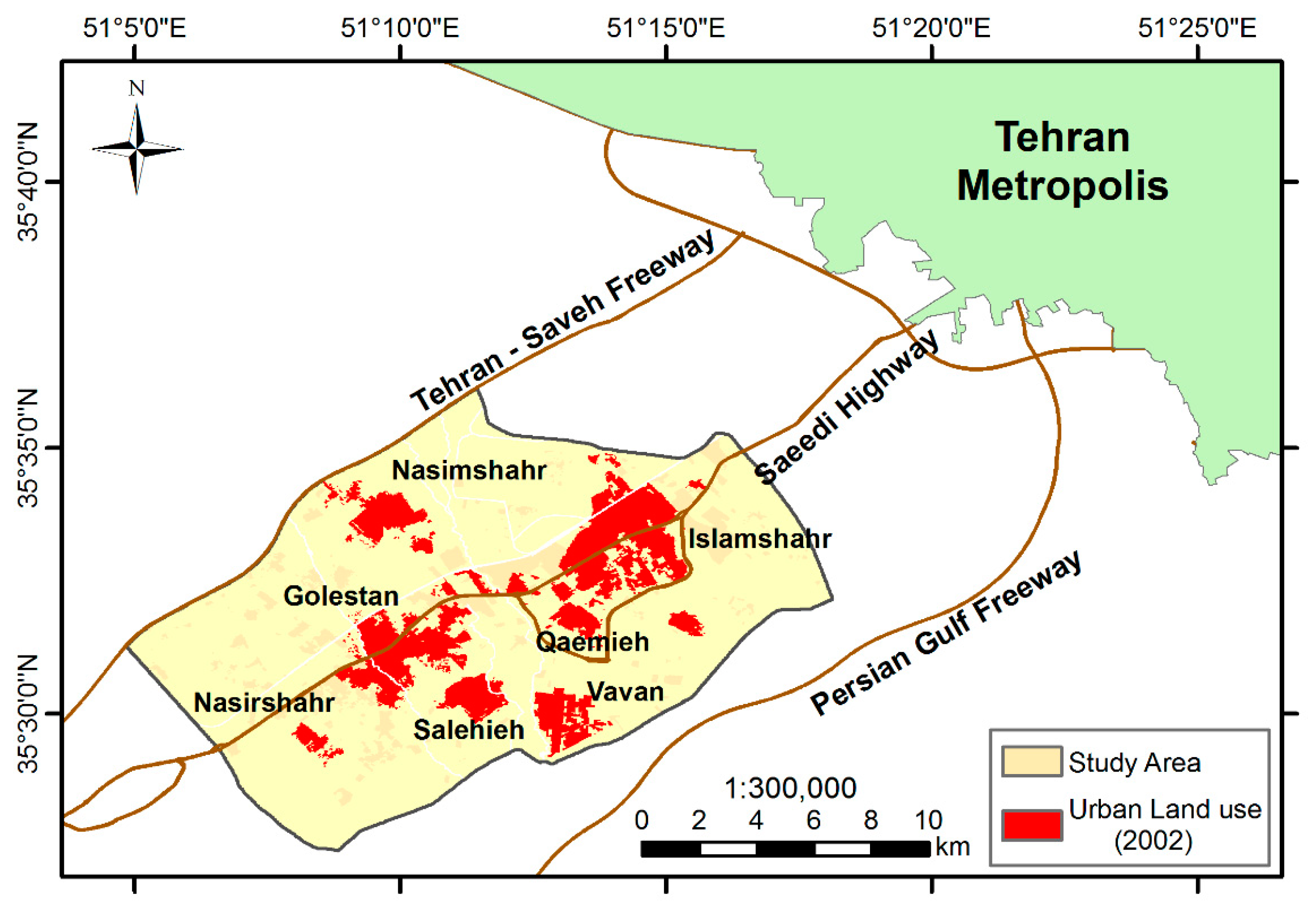
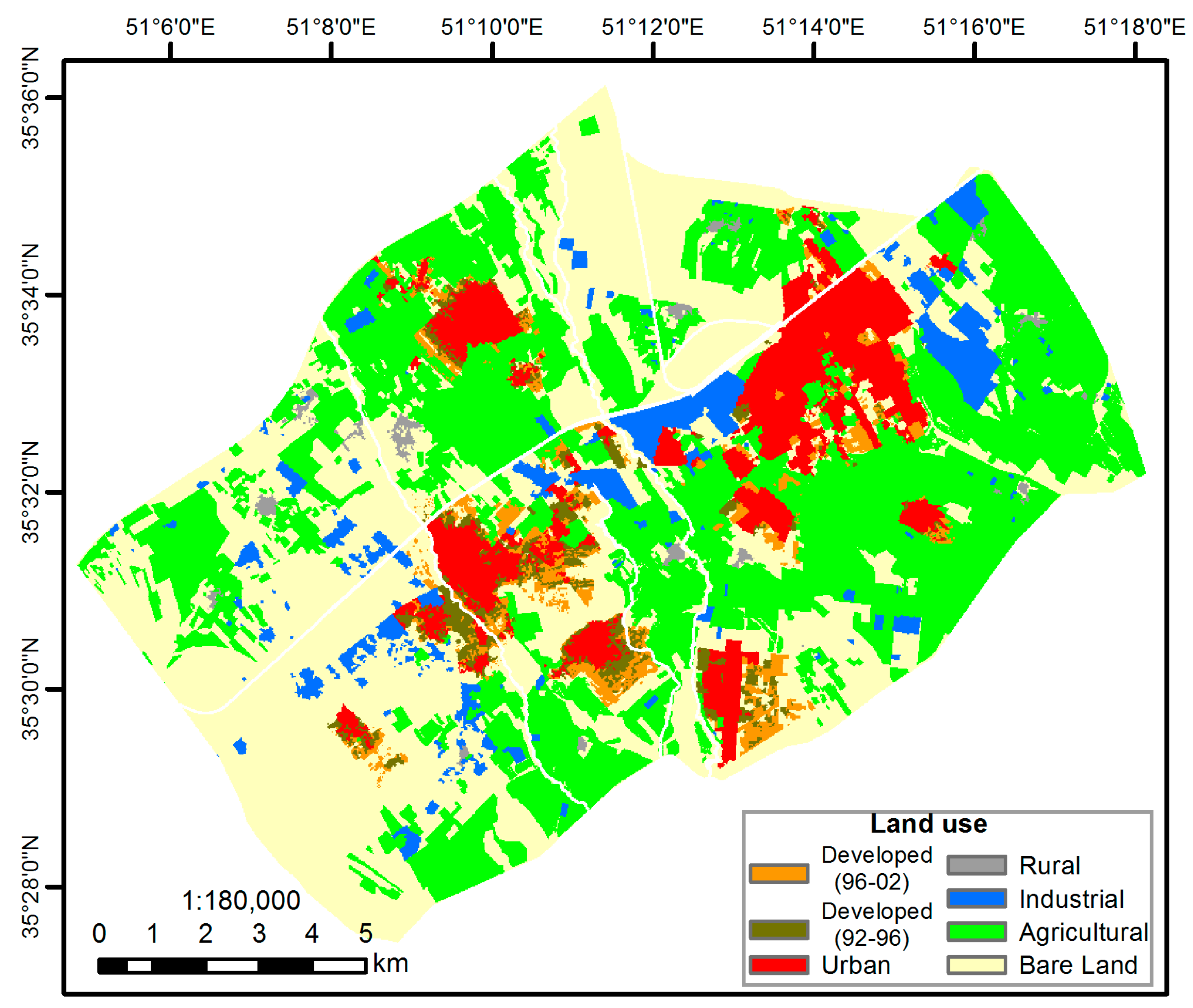
2. Study Area
3. Materials and Methods
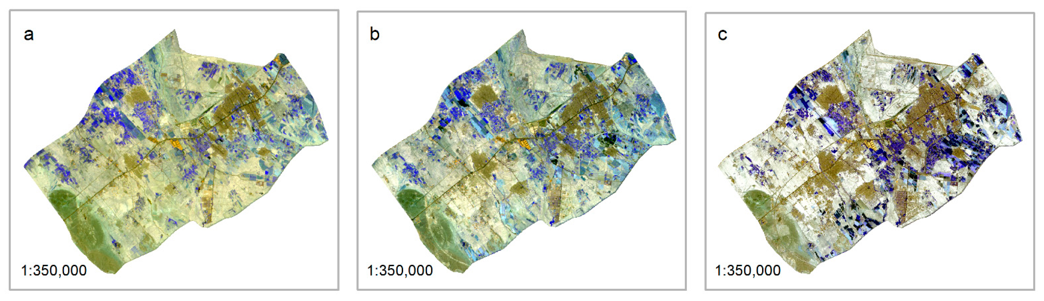
3.1. Data and Variables
3.2. Methodology
3.2.1. Research Outline
3.2.2. Global Support Vector Machines
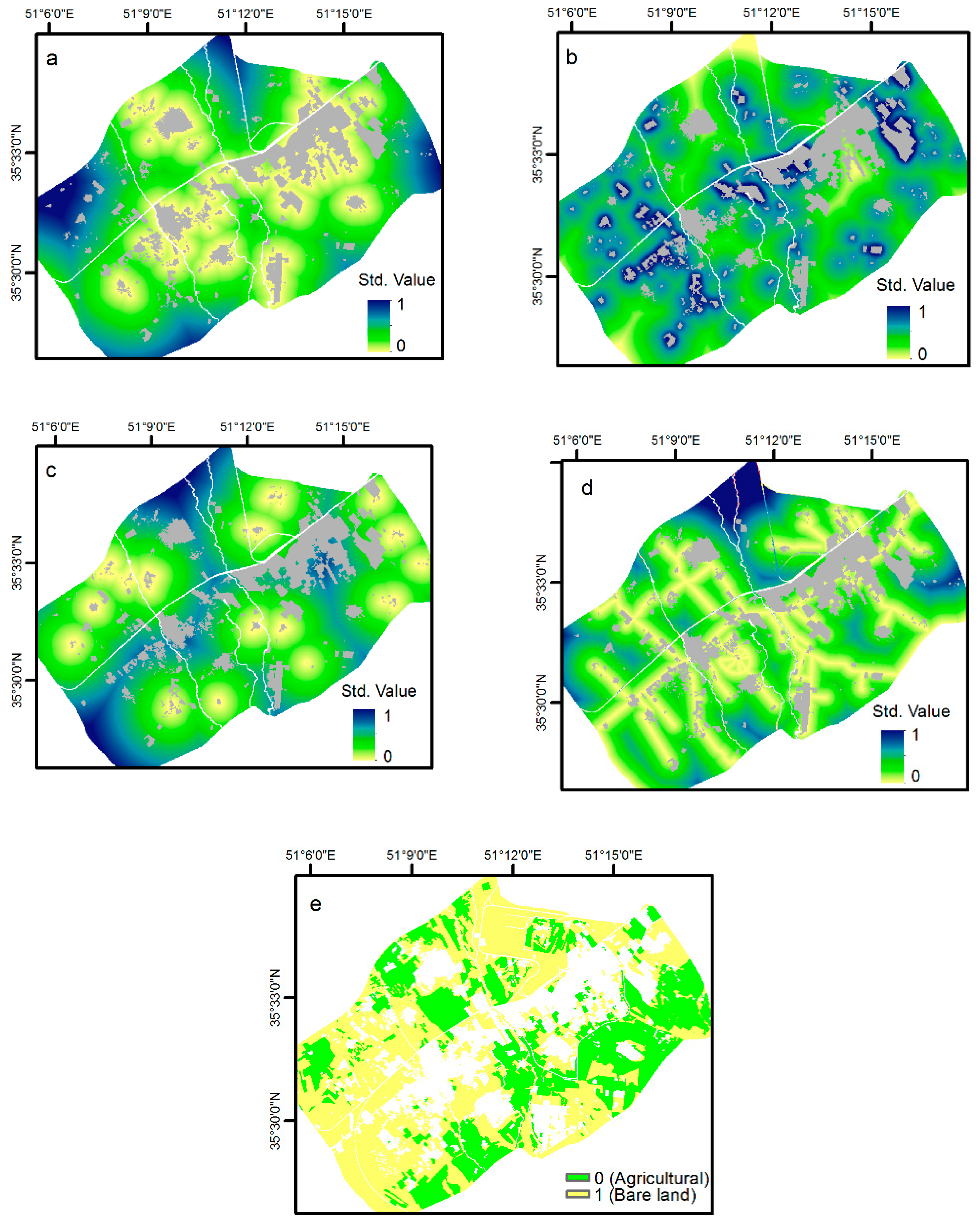
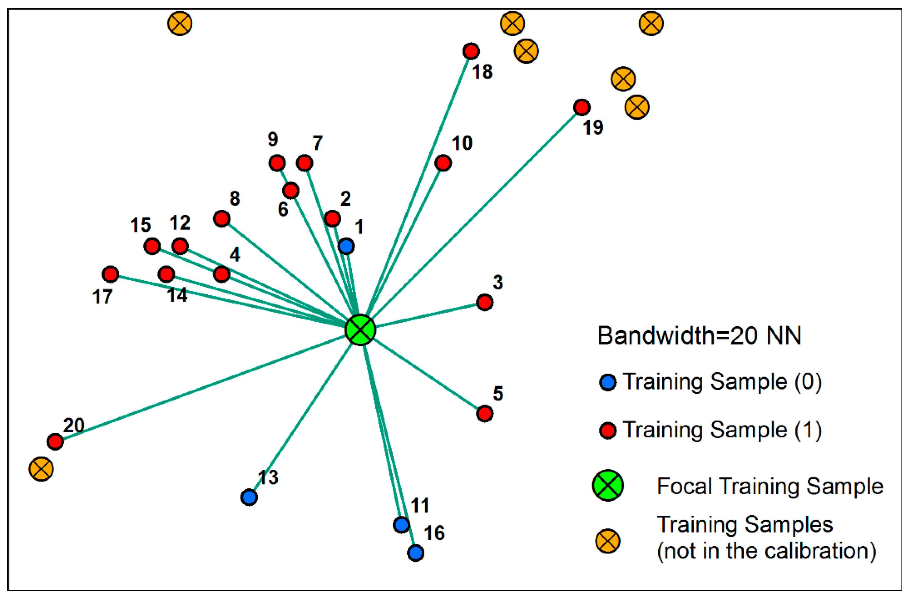
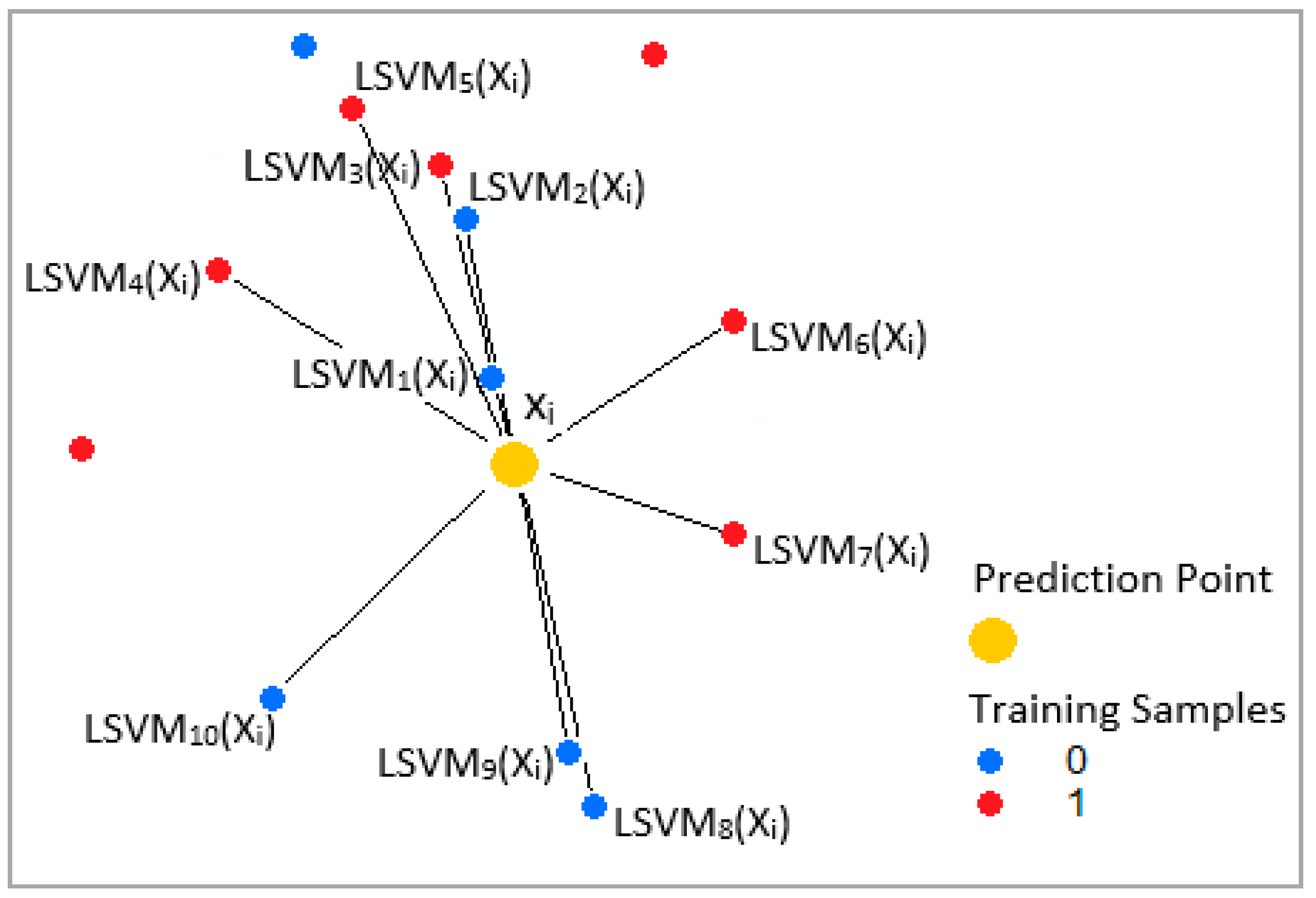
3.2.3. Local Support Vector Machines
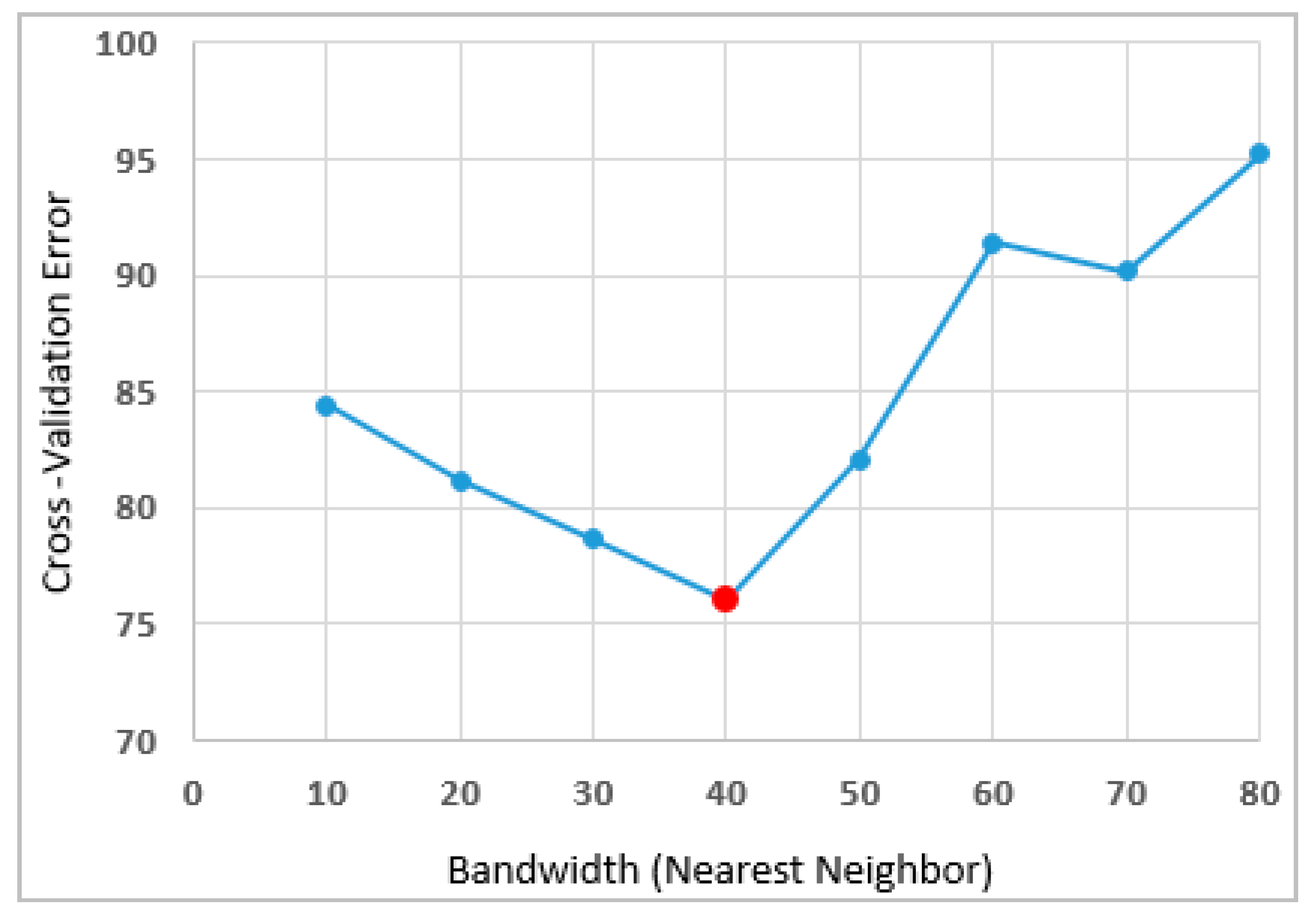
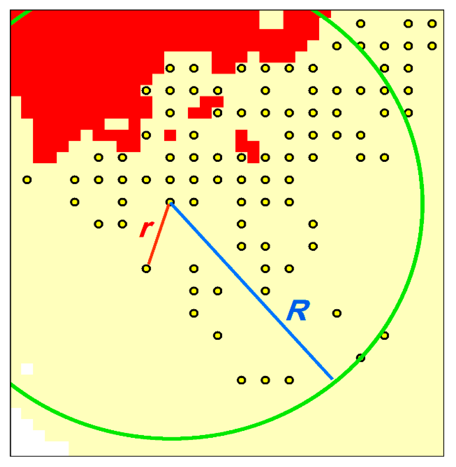
Determining the Optimal Bandwidth
Estimation
3.2.4. Integration of the Local and Global Models
3.2.5. Urban Cellular Automata
3.2.6. Validation
Area Under the ROC curve
Kappa Coefficient
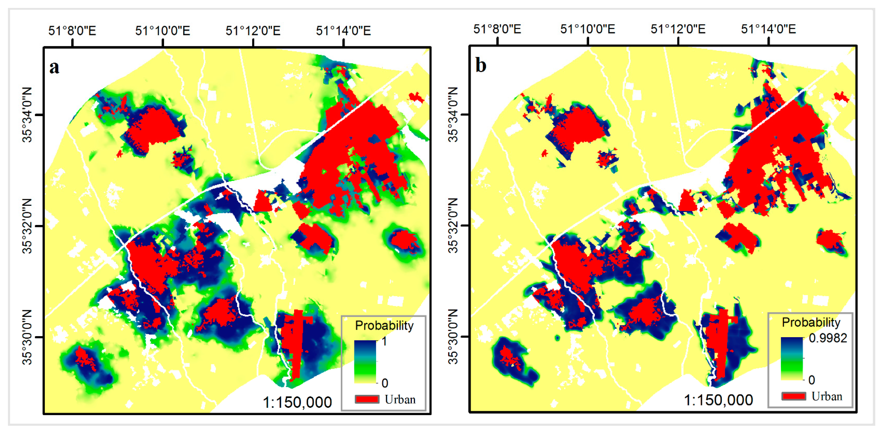
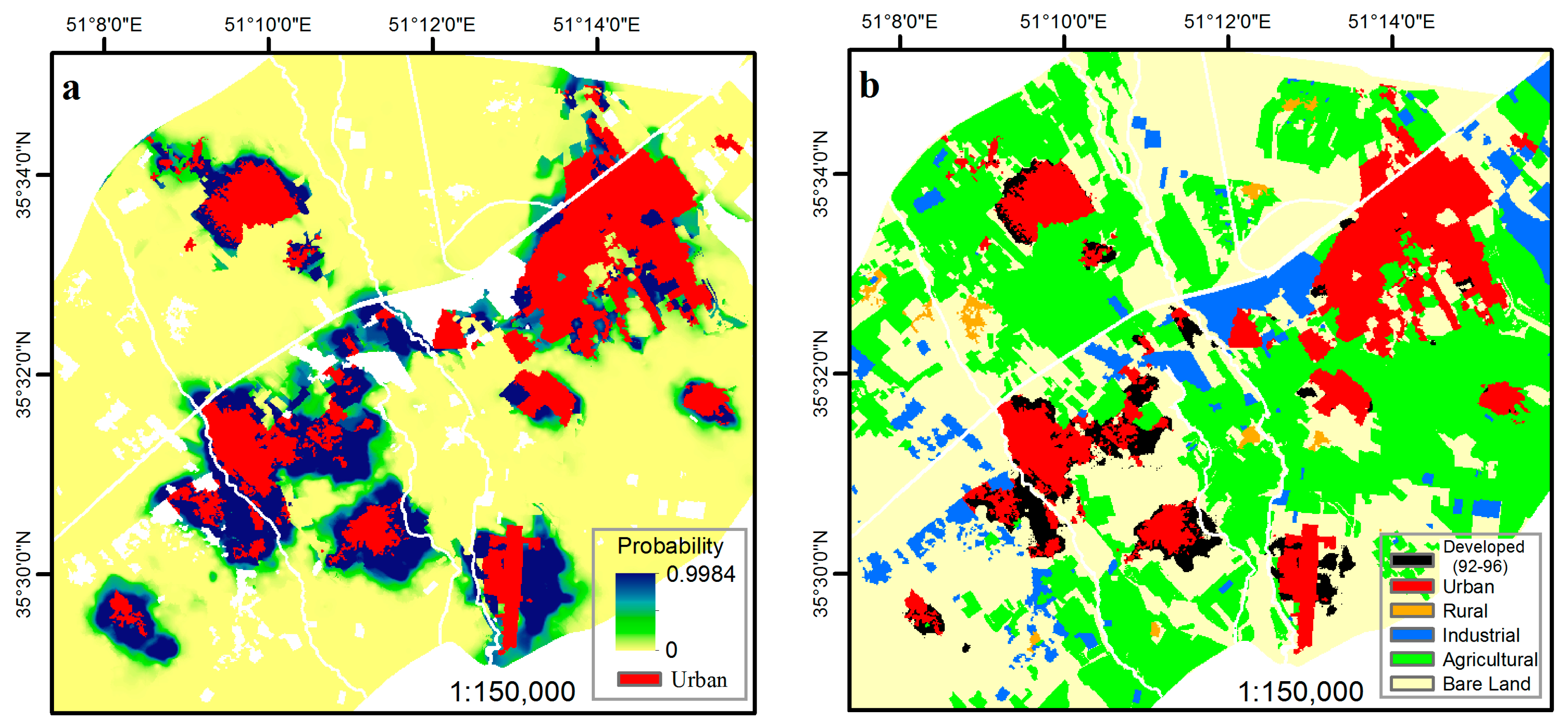
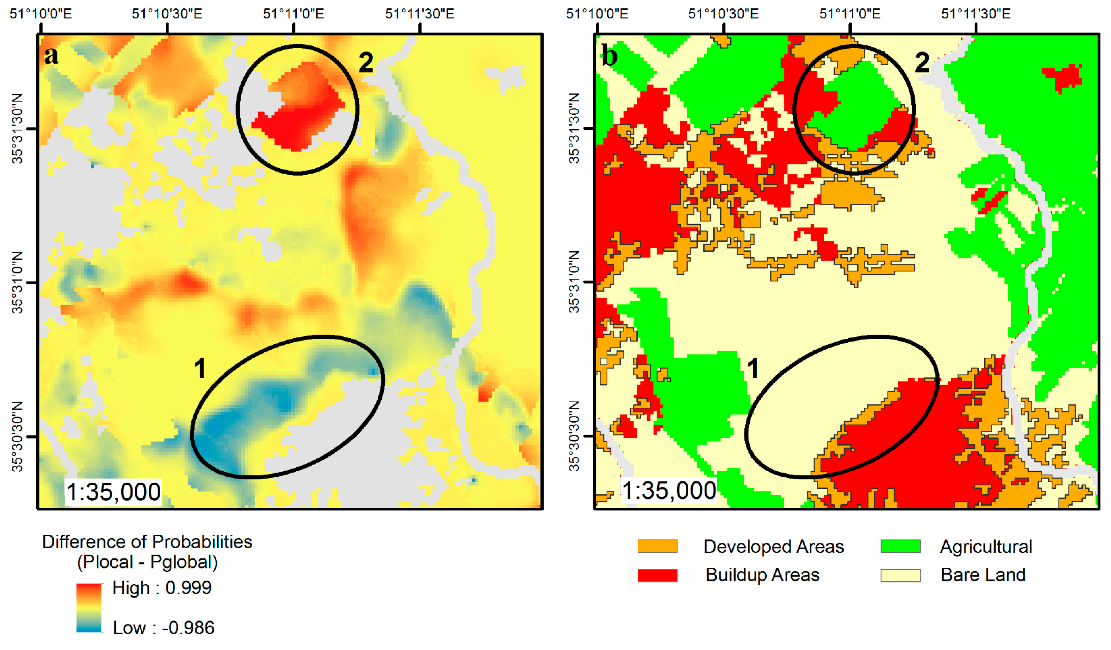
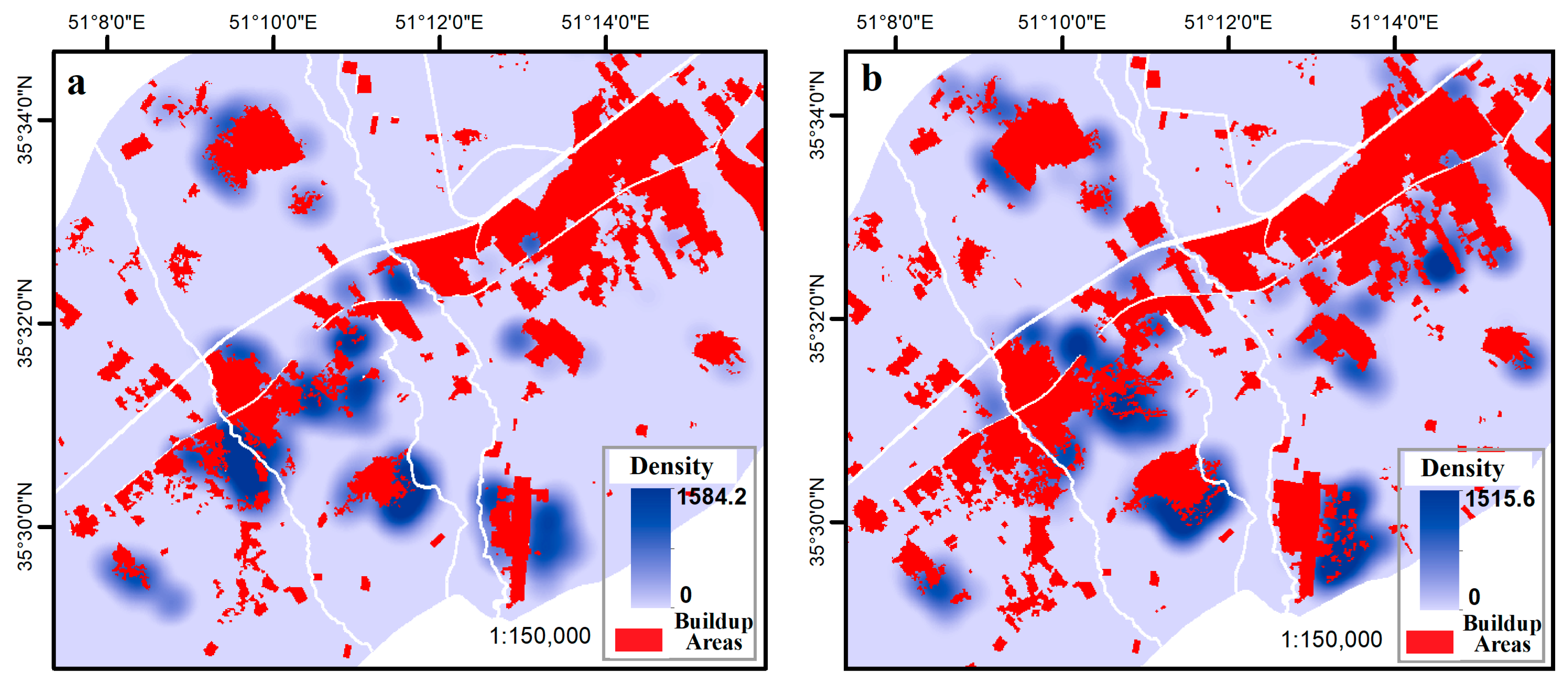
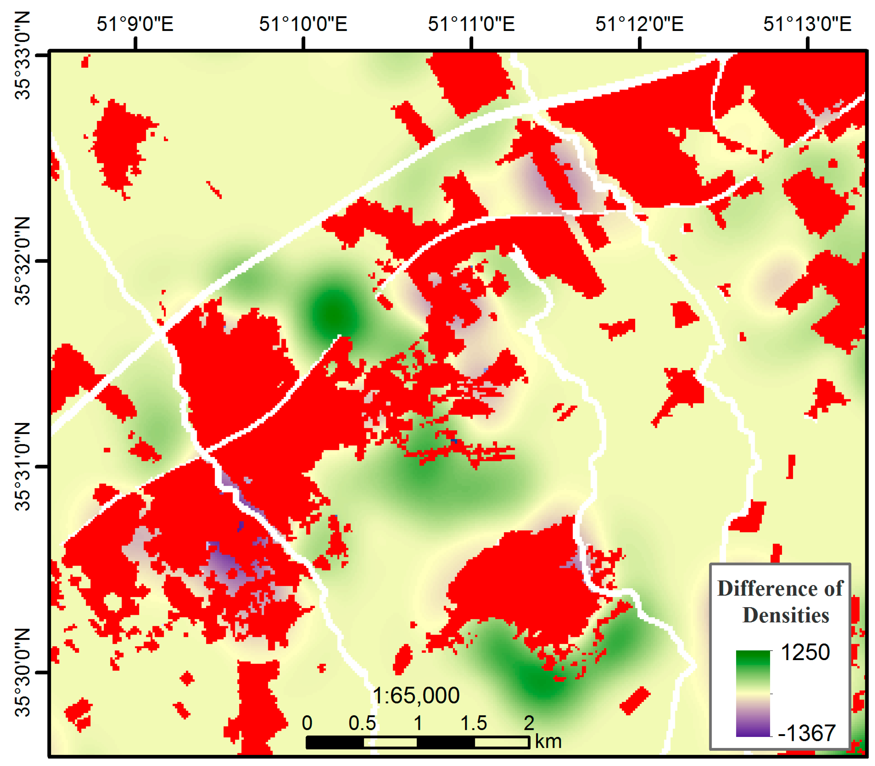
4. Results
5. Discussion
6. Conclusions
Author Contributions
Funding
Conflicts of Interest
References
- Liu, Y. Modelling Urban Development with Geographical Information Systems and Cellular Automata; CRC Press: Boca Raton, FL, USA, 2008; p. 1. ISBN 1-4200-5989-0. [Google Scholar]
- Pacione, M. Urban Geography: A Global Perspective, 3rd ed.; Routledge: Abingdon-on-Thames, UK, 2009; p. 164. ISBN 041546202. [Google Scholar]
- Bathrellos, G.D.; Gaki-Papanastassiou, K.; Skilodimou, H.D.; Papanastassiou, D.; Chousianitis, K.G. Potential suitability for urban planning and industry development using natural hazard maps and geological–geomorphological parameters. Environ. Earth. Sci. 2012, 66, 537–548. [Google Scholar] [CrossRef]
- Bathrellos, G.D.; Skilodimou, H.D.; Chousianitis, K.; Youssef, A.M.; Pradhan, B. Suitability estimation for urban development using multi-hazard assessment map. Sci. Total Environ. 2017, 575, 119–134. [Google Scholar] [CrossRef] [PubMed]
- Comber, A.; Brunsdon, C.; Green, E. Using a GIS-based network analysis to determine urban greenspace accessibility for different ethnic and religious groups. Landsc. Urban Plan. 2008, 86, 103–114. [Google Scholar] [CrossRef] [Green Version]
- Long, H.; Liu, Y.; Hou, X.; Li, T.; Li, Y. Effects of land use transitions due to rapid urbanization on ecosystem services: Implications for urban planning in the new developing area of China. Habitat. Int. 2014, 44, 536–544. [Google Scholar] [CrossRef]
- Papadopoulou-Vrynioti, K.; Bathrellos, G.D.; Skilodimou, H.D.; Kaviris, G.; Makropoulos, K. Karst collapse susceptibility mapping considering peak ground acceleration in a rapidly growing urban area. Eng. Geol. 2013, 158, 77–88. [Google Scholar] [CrossRef]
- Yeh, A.G.O.; Li, X. A cellular automata model to simulate development density for urban planning. Environ. Plann. B 2002, 29, 431–450. [Google Scholar] [CrossRef]
- Cao, M.; Bennett, S.J.; Shen, Q.; Xu, R. A bat-inspired approach to define transition rules for a cellular automaton model used to simulate urban expansion. Int. J. Geogr. Inf. Sci. 2016, 30, 1961–1979. [Google Scholar] [CrossRef]
- Clarke, K.C.; Hoppen, S.; Gaydos, L. A self-modifying cellular automaton model of historical urbanization in the San Francisco Bay area. Environ. Plan. B 1997, 24, 247–261. [Google Scholar] [CrossRef] [Green Version]
- He, J.; Li, X.; Yao, Y.; Hong, Y.; Jinbao, Z. Mining transition rules of cellular automata for simulating urban expansion by using the deep learning techniques. Int. J. Geogr. Inf. Sci. 2018, 32, 2076–2097. [Google Scholar] [CrossRef]
- Kamusoko, C.; Gamba, J. Simulating urban growth using a Random Forest-Cellular Automata (RF-CA) model. ISPRS Int. J. Geo-Inf. 2015, 4, 447–470. [Google Scholar] [CrossRef]
- Kocabas, V.; Dragicevic, S. Coupling Bayesian networks with GIS-based cellular automata for modeling land use change. In Proceedings of the International Conference on Geographic Information Science, Münster, Germany, 27–30 September 2006; pp. 217–233. [Google Scholar]
- Li, X.; Yeh, A.G.O. Calibration of cellular automata by using neural networks for the simulation of complex urban systems. Environ. Plan. A 2001, 33, 1445–1462. [Google Scholar] [CrossRef]
- Liu, X.; Li, X.; Shi, X.; Zhang, X.; Chen, Y. Simulating land-use dynamics under planning policies by integrating artificial immune systems with cellular automata. Int. J. Geogr. Inf. Sci. 2010, 24, 783–802. [Google Scholar] [CrossRef]
- Rimal, B.; Zhang, L.; Keshtkar, H.; Haack, B.N.; Rijal, S.; Zhang, P. Land use/Land cover dynamics and modeling of urban land expansion by the integration of cellular automata and markov chain. ISPRS Int. J. Geo-Inf. 2018, 7, 154. [Google Scholar] [CrossRef]
- Wu, F. Calibration of stochastic cellular automata: The application to rural-urban land conversions. Int. J. Geogr. Inf. Sci. 2002, 16, 795–818. [Google Scholar] [CrossRef]
- Yang, J.; Su, J.; Chen, F.; Xie, P.; Ge, Q. A local land use competition cellular automata model and its application. ISPRS Int. J. Geo-Inf. 2016, 5, 106. [Google Scholar] [CrossRef]
- Yao, Y.; Li, J.; Zhang, X.; Duan, P.; Li, S.; Xu, Q. Investigation on the expansion of urban construction land use based on the CART-CA model. ISPRS Int. J. Geo-Inf. 2017, 6, 149. [Google Scholar] [CrossRef]
- McDonald, R.I.; Urban, D.L. Spatially varying rules of landscape change: Lessons from a case study. Landsc. Urban Plan. 2006, 74, 7–20. [Google Scholar] [CrossRef]
- Meentemeyer, R.K.; Tang, W.; Dorning, M.A.; Vogler, J.B.; Cunniffe, N.J.; Shoemaker, D.A. FUTURES: Multilevel simulations of emerging urban–rural landscape structure using a stochastic patch-growing algorithm. Ann. Assoc. Am. Geogr. 2013, 103, 785–807. [Google Scholar] [CrossRef]
- Brunsdon, C.; Fotheringham, A.S.; Charlton, M.E. Geographically weighted regression: A method for exploring spatial nonstationarity. Geogr. Anal. 1996, 28, 281–298. [Google Scholar] [CrossRef]
- Lloyd, C.D. Local Models for Spatial Analysis, 2nd ed.; CRC Press: Boca Raton, FL, USA, 2010; ISBN 978-1-4398-2919-6. [Google Scholar]
- Kazemzadeh-Zow, A.; Zanganeh Shahraki, S.; Salvati, L.; Samani, N.N. A spatial zoning approach to calibrate and validate urban growth models. Int. J. Geogr. Inf. Sci. 2016, 31, 763–782. [Google Scholar] [CrossRef]
- Li, X.; Liu, X. An extended cellular automaton using case-based reasoning for simulating urban development in a large complex region. Int. J. Geogr. Inf. Sci. 2006, 20, 1109–1136. [Google Scholar] [CrossRef]
- Li, X.; Yang, Q.; Liu, X. Discovering and evaluating urban signatures for simulating compact development using cellular automata. Landsc. Urban Plan. 2008, 86, 177–186. [Google Scholar] [CrossRef]
- Mirbagheri, B.; Alimohammadi, A. Improving urban cellular automata performance by integrating global and geographically weighted logistic regression models. Trans. GIS 2017, 21, 1280–1297. [Google Scholar] [CrossRef]
- Shu, B.; Bakker, M.M.; Zhang, H.; Li, Y.; Qin, W.; Carsjens, G.J. Modeling urban expansion by using variable weights logistic cellular automata: A case study of Nanjing, China. Int. J. Geogr. Inf. Sci. 2017, 31, 1314–1333. [Google Scholar] [CrossRef]
- Anselin, L. Local indicators of spatial association-LISA. Geogr. Anal. 1995, 27, 93–115. [Google Scholar] [CrossRef]
- Getis, A.; Ord, J.K. The analysis of spatial association by use of distance statistics. Geogr. Anal. 1992, 24, 189–206. [Google Scholar] [CrossRef]
- Fotheringham, A.S.; Brunsdon, C.; Charlton, M. Geographically Weighted Regression: The Analysis of Spatially Varying Relationships; Wiley: New York, NY, USA, 2002; ISBN 0471496162. [Google Scholar]
- Gao, J.; Li, S. Detecting spatially non-stationary and scale-dependent relationships between urban landscape fragmentation and related factors using geographically weighted regression. Appl. Geogr. 2011, 31, 292–302. [Google Scholar] [CrossRef]
- Ivajnšič, D.; Kaligarič, M.; Žiberna, I. Geographically weighted regression of the urban heat island of a small city. Appl. Geogr. 2014, 53, 341–353. [Google Scholar] [CrossRef]
- Kumari, M.; Singh, C.K.; Bakimchandra, O.; Basistha, A. Geographically weighted regression based quantification of rainfall–topography relationship and rainfall gradient in Central Himalayas. Int. J. Climatol. 2017, 37, 1299–1309. [Google Scholar] [CrossRef]
- Shariat-Mohaymany, A.; Shahri, M.; Mirbagheri, B.; Matkan, A.A. Exploring Spatial Non-Stationarity and Varying Relationships between Crash Data and Related Factors Using Geographically Weighted Poisson Regression. Trans. GIS 2014, 19, 321–337. [Google Scholar] [CrossRef]
- Luo, J.; Kanala, N.K. Modeling urban growth with geographically weighted multinomial logistic regression. In Proceedings of the Geoinformatics 2008 and Joint Conference on GIS and Built Environment: The Built Environment and Its Dynamics, Guangzhou, China, 28–29 June 2008. [Google Scholar]
- Luo, J.; Wei, Y.H. Modeling spatial variations of urban growth patterns in Chinese cities: The case of Nanjing. Landsc. Urban Plan. 2009, 91, 51–64. [Google Scholar] [CrossRef]
- Nakaya, T. Geographically weighted generalised linear modelling. In Geocomputation A Practical Primer; Brunsdon, C., Singleton, A., Eds.; Sage Publication: London, UK, 2015; p. 195. ISBN 1446272931. [Google Scholar]
- Shafizadeh-Moghadam, H.; Helbich, M. Spatiotemporal variability of urban growth factors: A global and local perspective on the megacity of Mumbai. Int. J. Appl. Earth. Obs. 2015, 35, 187–198. [Google Scholar] [CrossRef]
- Gilardi, N.; Bengio, S. Local machine learning models for spatial data analysis. J. Geogr. Inform. Decis. Anal. 2001, 4, 11–28. [Google Scholar]
- Martens, D.; Baesens, B.; Van Gestel, T.; Vanthienen, J. Comprehensible credit scoring models using rule extraction from support vector machines. Eur. J. Oper. Res. 2007, 183, 1466–1476. [Google Scholar] [CrossRef]
- Okwuashi, O.; Mcconchie, J.; Nwilo, P.; Eyo, E. Stochastic GIS cellular automata for land use change simulation: Application of a kernel based model. In Proceedings of the 10th International Conference on GeoComputation, Sydney, Australia, 30 November–2 December 2009; pp. 1–7. [Google Scholar]
- Rienow, A.; Goetzke, R. Supporting SLEUTH–Enhancing a cellular automaton with support vector machines for urban growth modeling. Comput. Environ. Urban 2016, 49, 66–81. [Google Scholar] [CrossRef]
- Yang, Q.; Li, X.; Shi, X. Cellular automata for simulating land use changes based on support vector machines. Comput. Geosci. 2008, 34, 592–602. [Google Scholar] [CrossRef]
- Bottou, L.; Vapnik, V. Local learning algorithms. Neural Comput. 1992, 4, 888–900. [Google Scholar] [CrossRef]
- Ralaivola, L.; D’alché-Buc, F. Incremental support vector machine learning: A local approach. In Proceedings of the International Conference on Artificial Neural Networks, Vienna, Austria, 9–13 August 2001; pp. 322–330. [Google Scholar]
- Yang, X.; Song, Q.; Wang, Y. A weighted support vector machine for data classification. Int. J. Pattern Recogn. 2007, 21, 961–976. [Google Scholar] [CrossRef]
- Cheng, H.; Tan, P.N.; Jin, R. Localized support vector machine and its efficient algorithm. In Proceedings of the SIAM International Conference on Data Mining, Minneapolis, MN, USA, 30 April–1 May 2007; pp. 461–466. [Google Scholar]
- Cheng, H.; Tan, P.N.; Jin, R. Efficient algorithm for localized support vector machine. IEEE. Trans. Knowl. Data Eng. 2010, 22, 537–549. [Google Scholar] [CrossRef]
- Ladicky, L.; Torr, P. Locally linear support vector machines. In Proceedings of the 28th International Conference on Machine Learning (ICML-11), Bellevue, WA, USA, 19–24 June 2011; pp. 985–992. [Google Scholar]
- Gu, Q.; Han, J. Clustered Support Vector Machines. In Proceedings of the Sixteenth International Conference on Artificial Intelligence and Statistics, Scottsdale, AZ, USA, 29 April–1 May 2013; pp. 307–315. [Google Scholar]
- Andris, C.; Cowen, D.; Wittenbach, J. Support vector machine for spatial variation. Trans. GIS 2013, 17, 41–61. [Google Scholar] [CrossRef]
- Nazarian, A. Urban sprawl of Tehran city and emergence of satellite towns. J. Geogr. Res. 1991, 6, 97–139. [Google Scholar]
- Pourahmad, A.; Seifoddini, F.; Parnoon, Z. Migration and land use change in Islamshahr city. J. Geogr. Stud. Arid Reg. 2011, 2, 131–150. [Google Scholar]
- Ghamami, M. Urban Agglomeration of Tehran and Around Cities; Center of Studies and Researchers of Iran’s Architecture and Urban Planning; Ministry of Roads and Urban Development: Tehran, Iran, 2000. [Google Scholar]
- Gunn, S.R. Support vector machines for classification and regression. ISIS Tech. Rep. 1998, 14, 85–86. [Google Scholar]
- Kanevski, M.; Pozdnoukhov, A.; Timonin, V. Machine Learning for Spatial Environmental Data: Theory, Applications and Software; Epfl Press: Lausanne, Switzerland, 2009; p. 255. ISBN 978-2-940222-24-7.
- Pal, M.; Foody, G.M. Feature selection for classification of hyperspectral data by SVM. IEEE. Trans. Geosci. Remote 2010, 48, 2297–2307. [Google Scholar] [CrossRef]
- Vapnik, V.N.; Chervonenkis, A.Y. On the uniform convergence of relative frequencies of events to their probabilities. In Measures of Complexity; Vovk, V., Gammerman, A., Papadopoulos, H., Eds.; Springer: New York, NY, USA, 2015; pp. 11–30. ISBN 3319218514. [Google Scholar]
- Vapnik, V. The Nature of Statistical Learning Theory; Springer: New York, NY, USA, 2000; p. 139. ISBN 0387987800. [Google Scholar]
- Cortes, C.; Vapnik, V. Support-vector networks. Mach. Learn. 1995, 20, 273–297. [Google Scholar] [CrossRef] [Green Version]
- Bousquet, O.; Pez-Cruz, F. Kernel methods and their applications to signal processing. In Proceedings of the IEEE International Conference on Acoustics, Speech, and Signal Processing, Hong Kong, China, 6–10 April 2003. [Google Scholar]
- Chang, C.C.; Lin, C.J. LIBSVM: A library for support vector machines. ACM Trans. Intell. Syst. Technol. 2011, 2, 27. [Google Scholar] [CrossRef]
- Platt, J. Probabilistic outputs for support vector machines and comparisons to regularized likelihood methods. In Advances in Large Margin Classifiers; Smola, A.J., Bartlett, P., Schölkopf, B., Schuurmans, D., Eds.; MIT Press: Cambridge, MA, USA, 1999; Volume 10, pp. 61–74. [Google Scholar]
- Kohavi, R. A study of cross-validation and bootstrap for accuracy estimation and model selection. In Proceedings of the International Joint Conference on Artificial Intelligence, Montreal, QC, Canada, 9–15 August 1995; pp. 1137–1145. [Google Scholar]
- Olson, D.L.; Delen, D. Advanced Data Mining Techniques; Springer: Berlin, Germany, 2008; p. 157. ISBN 3540769161. [Google Scholar]
- Frohlich, H.; Zell, A. Efficient parameter selection for support vector machines in classification and regression via model-based global optimization. In Proceedings of the International Joint Conference on Neural Networks, Montreal, QC, Canada, 31 July–4 August 2005; pp. 1431–1436. [Google Scholar]
- Cleveland, W.S. Robust locally weighted regression and smoothing scatterplots. J. Am. Stat. Assoc. 1979, 74, 829–836. [Google Scholar] [CrossRef]
- Liao, J.; Tang, L.; Shao, G.; Su, X.; Chen, D.; Xu, T. Incorporation of extended neighborhood mechanisms and its impact on urban land-use cellular automata simulations. Environ. Model. Softw. 2016, 75, 163–175. [Google Scholar] [CrossRef]
- Verstegen, J.A.; Karssenberg, D.; Van Der Hilst, F.; Faaij, A.P. Identifying a land use change cellular automaton by Bayesian data assimilation. Environ. Model. Softw. 2014, 53, 121–136. [Google Scholar] [CrossRef]
- White, R.; Engelen, G. High-resolution integrated modelling of the spatial dynamics of urban and regional systems. Comput. Environ. Urban 2000, 24, 383–400. [Google Scholar] [CrossRef] [Green Version]
- Feng, Y.; Liu, M.; Chen, L.; Liu, Y. Simulation of dynamic urban growth with partial least squares regression-based cellular automata in a GIS environment. ISPRS Int. J. Geo-Inf. 2016, 5, 243. [Google Scholar] [CrossRef]
- Gorsevski, P.V.; Onasch, C.M.; Farver, J.R.; Ye, X. Detecting grain boundaries in deformed rocks using a cellular automata approach. Comput. Geosci. 2012, 42, 136–142. [Google Scholar] [CrossRef]
- White, R.; Engelen, G. Cellular automata and fractal urban form: A cellular modelling approach to the evolution of urban land-use patterns. Environ. Plan. A 1993, 25, 1175–1195. [Google Scholar] [CrossRef]
- Hu, Z.; Lo, C. Modeling urban growth in Atlanta using logistic regression. Comput. Environ. Urban 2007, 31, 667–688. [Google Scholar] [CrossRef]
- Pontius, R.G.; Pacheco, P. Calibration and validation of a model of forest disturbance in the Western Ghats, India 1920–1990. GeoJournal 2004, 61, 325–334. [Google Scholar] [CrossRef]
- Delong, E.R.; Delong, D.M.; Clarke-Pearson, D.L. Comparing the areas under two or more correlated receiver operating characteristic curves: A nonparametric approach. Biometrics 1988, 837–845. [Google Scholar] [CrossRef]
- De Smith, M.J.; Goodchild, M.F.; Longley, P. Geospatial Analysis: A Comprehensive Guide to Principles, Techniques and Software Tools; Troubador Publishing Ltd.: Leicester, UK, 2007; pp. 126–133. ISBN 1-905886-60-8. [Google Scholar]


| Satellite Image | Acquisition Date | Spatial Resolution (Meters) |
|---|---|---|
| SPOT 2 | 25 June 1992 | 20 |
| SPOT 3 | 19 June 1996 | 20 |
| SPOT 4 | 13 July 2002 | 10 |
| σ | −6 | −5 | −4 | −3 | −2 | |
|---|---|---|---|---|---|---|
| C | ||||||
| 0.125 | 21.88 | 22.10 | 22.01 | 23.19 | 25.90 | |
| 0.25 | 21.89 | 18.97 | 18.58 | 21.22 | 24.95 | |
| 0.5 | 22.42 | 15.74 | 15.93 | 19.36 | 23.47 | |
| 1 | 27.95 | 15.23 | 14.78 | 18.19 | 22.12 | |
| 2 | 61.18 | 16.52 | 14.86 | 17.20 | 20.70 | |
| 4 | 98.36 | 18.20 | 15.49 | 16.57 | 19.58 | |
| 8 | 71.07 | 25.06 | 15.92 | 16.29 | 19.17 | |
| GSVM (WLocal = 0) | WLocal | LSVM (WLocal = 1) | |||||||||
|---|---|---|---|---|---|---|---|---|---|---|---|
| 0.1 | 0.2 | 0.3 | 0.4 | 0.5 | 0.6 | 0.7 | 0.8 | 0.9 | |||
| AUC | 0.979 | 0.987 | 0.988 | 0.989 | 0.990 | 0.990 | 0.990 | 0.990 | 0.990 | 0.989 | 0.987 |
| Kappa | 0.489 | 0.578 | 0.619 | 0.642 | 0.660 | 0.667 | 0.670 | 0.667 | 0.660 | 0.657 | 0.617 |
| 1992–1996 | 1996–2002 | ||||
|---|---|---|---|---|---|
| Models | LGSVM vs. GSVM | LGSVM vs. LSVM | LGSVM vs. GSVM | LGSVM vs. LSVM | |
| Statistics | |||||
| Difference in AUCs | 0.0104 | 0.00308 | 0.0479 | 0.00403 | |
| Standard error (DeLong et al. 1988) | 0.000238 | 0.000238 | 0.00144 | 0.000483 | |
| z statistic | 43.513 | 12.951 | 33.26 | 8.33 | |
| Significance level | p-value < 0.001 | p-value < 0.001 | p-value < 0.001 | p-value < 0.001 | |
| Model | AUC | Model | Kappa |
|---|---|---|---|
| GSVM | 0.896 | GSVM-CA | 0.483 |
| LSVM | 0.939 | LSVM-CA | 0.493 |
| LGSVM | 0.943 | LGSVM-CA | 0.512 |
| Density of Urban Development | ||
|---|---|---|
| 1992–1996 | 1996–2002 | |
| PGSVM | 0.712▲ | 0.567▼ |
| PLSVM | 0.787▲ | 0.662▼ |
| PLGSVM | 0.792▲ | 0.673▼ |
© 2018 by the authors. Licensee MDPI, Basel, Switzerland. This article is an open access article distributed under the terms and conditions of the Creative Commons Attribution (CC BY) license (http://creativecommons.org/licenses/by/4.0/).
Share and Cite
Mirbagheri, B.; Alimohammadi, A. Integration of Local and Global Support Vector Machines to Improve Urban Growth Modelling. ISPRS Int. J. Geo-Inf. 2018, 7, 347. https://doi.org/10.3390/ijgi7090347
Mirbagheri B, Alimohammadi A. Integration of Local and Global Support Vector Machines to Improve Urban Growth Modelling. ISPRS International Journal of Geo-Information. 2018; 7(9):347. https://doi.org/10.3390/ijgi7090347
Chicago/Turabian StyleMirbagheri, Babak, and Abbas Alimohammadi. 2018. "Integration of Local and Global Support Vector Machines to Improve Urban Growth Modelling" ISPRS International Journal of Geo-Information 7, no. 9: 347. https://doi.org/10.3390/ijgi7090347
APA StyleMirbagheri, B., & Alimohammadi, A. (2018). Integration of Local and Global Support Vector Machines to Improve Urban Growth Modelling. ISPRS International Journal of Geo-Information, 7(9), 347. https://doi.org/10.3390/ijgi7090347