Article

A Novel Approach for Identifying Urban Built-Up Area Boundaries Using High-Resolution Remote-Sensing Data Based on the Scale Effect

1
Institute of Remote Sensing and Digital Earth, Chinese Academy of Sciences, Beijing 100101, China
2
University of Chinese Academy of Sciences, Beijing 100101, China
*
Authors to whom correspondence should be addressed.
ISPRS Int. J. Geo-Inf. 2018, 7(4), 135; https://doi.org/10.3390/ijgi7040135
Submission received: 7 March 2018 / Revised: 21 March 2018 / Accepted: 26 March 2018 / Published: 1 April 2018

Abstract

:
Identifying urban built-up area boundaries is critical to urban data statistics, size measurement, and spatial control. However, previous methods of extracting urban built-up area boundaries based on low-resolution remote-sensing data are frequently constrained by data accuracy. In this paper, a new method for extracting urban built-up area boundaries using high-resolution remote sensing images based on scale effects is proposed. Firstly, we generate a number of different levels of edge-multiplied hexagonal vector grids. Secondly, the impervious surface densities are calculated based on the hexagonal vector grids with the longest edge. Then, the hexagonal grids with higher impervious surface densities are extracted as the built-up area of the first level. Thirdly, we gradually reduce the spatial scale of the hexagonal vector grid and repeat the extraction process based on the extracted built-up area in the previous step. Eventually, we obtain the urban built-up area boundary at the smallest scale. Plausibility checks indicate that the suggested method not only guarantees the spatial continuity of the resultant urban built-up area boundary, but also highlights the prevailing orientation of urban expansion. The extracted Beijing built-up area boundary can serve as a reference in decision-making for space planning and land-use control.

1. Introduction

Unchecked and unmanaged urban growth has been attributed to lack of adoption of efficient and effective urban planning tools. Some countries control urban sprawl by delineating urban built-up area boundaries, which provides foundational information for urban management and meets the requirements for urban pattern and urban spatial structure research [1]. However, defining city boundaries is invariably an enthralling challenge for urban geographers and planners [2]. There is little international consistency in what is defined as urban, and many countries recognize urban as including overflow and suburbs outside municipal limits, giving rise to additional definitions, such as urbanized areas, metropolitan areas, or mega-regions [3,4,5]. In fact, in urban areas, particularly at the rural-urban fringe, rural landscapes are blended with urban landscapes, and there are no rigid indices for discriminating the urban area from the rural area [6,7,8]. In China, urban administrative areas comprise the built-up area and the rural area within its jurisdiction. However, the urban statistics in China are based on the administrative unit and cannot accurately reflect the true state of urban built-up areas in China [3,9]. Further, such data are ineffective for comparing cities as the spatial units are spatially inconsistent [10,11]. Identifying the urban built-up area boundaries in China according to their characteristics is of great importance to urban data statistics, size measurement, land use, spatial control, and inter-city comparison [12]. This study focuses on the delimitation of urban landscapes by the parameter built-up area. Urban built-up area is commonly identified based on two key aspects. First, the urban built-up area should have relatively continuous impervious surface of high density to distinguish it from rural surface landscapes. Second, the urban built-up area should have a relatively high population density to distinguish it from rural cultural or economic activities. For fast-growing cities, population density is very high within the continuous impervious surfaces in China. Hence, we extract urban built-up area based on the relatively continuous impervious surfaces of high density in this study.
From the perspective of the data sources, current studies related to urban built-up area delimitation have mostly been based on demographical statistics [13,14,15,16], POI (point-of-interest) data [1], land cover classification [17,18,19,20] such as the Global Urban Footprint [21,22], and nighttime light [23,24,25]. From the perspective of data processing, methods of identifying urban built-up area can be grouped into two categories. The methods of the first group involve acquiring relatively continuous urban built-up areas using spatial search algorithms. Rozenfeld et al. (2008) developed a city cluster algorithm (CCA) that searches continuously populated areas on fine-scale geographical units and assigns them to urban built-up areas [26,27]. Chen et al. (2015) developed an urban dilation approach based on remote-sensing imagery data. In this approach, the search radius is established according to the scaling relationships between the neighboring range of pixels and the number of spatial clusters [28]. Although spatial search algorithms can easily yield the urban built-up area, defining the appropriate search conditions and search units is a challenge. Additionally, the process of extracting urban built-up area boundaries completely based on search algorithms is not transparent. It is also impossible to see how the boundaries are formed in the process of extraction. The methods of the second group involve extracting urban built-up area boundaries via threshold indicators. Some scholars have proposed some indices based on the spectral information or textural features of remote-sensing imagery, and then extracting the urban built-up area with the threshold value of those indices. For example, Zha et al. (2003) proposed a normalized difference built-up index (NDBI) to automate the process of mapping built-up areas [29]. Pesaresi et al. (2008) constructed a texture-derived built-up presence index (PanTex) based on fuzzy rule-based composition of anisotropic textural co-occurrence measures derived from the satellite data by the gray-level co-occurrence matrix (GLCM) [30]. Apart from indices related to remote-sensing data, the fractal dimension index based on fractal geometry has also been used to identify urban built-up area. Tannier et al. (2011) detected any multiscale spatial discontinuity of urban building blocks using the Minkowski dilation threshold based on fractal geography and extracted the morphological multiscale boundary of an urban agglomeration using the dilation threshold [2]. At present, big data obtained from web maps has also been used to extract urban built-up area based on threshold methods. Xu et al. (2016) generated a density contour through kernel density spatial interpolation using POI data to obtain the mutation point of the density contour-encircled area as a function of kernel density. They used this mutation point as the threshold for delimiting urban area boundaries [1]. In addition, some researchers have used multi-source geodata or composite indices to identify urban built-up areas. Jamal Abed et al. (2003) established a composite index compounding urban building concentration intensity, land-use abundance, economic activity intensity, and urbanization intensity together with remote-sensing imagery and GIS data, and identified the fuzzy urban built-up area boundaries based on the threshold of this composite index [19]. Georg et al. (2018) delimited the Boswash urban corridor using multi-source geodata (built-up extent, infrastructure and socioeconomic data) and set individual thresholds for each input layers based on the connectivity of the Boswash area [21]. The disadvantage of using threshold indictor to obtain urban built-up area boundaries arises from the fact that the threshold relies on the empirical knowledge of the researcher and the method cannot guarantee the continuity of the resultant urban built-up area boundary.
Spatial scale is a fundamental problem in geography [31]. Measurements with different scales of spatial units can produce significantly different results that vary from one another [32,33,34,35]. Geographically, rural settlements are present as small clusters scattered across the rural green space landscapes, while urban built-up area is present as large, relatively continuous impervious surface clusters. At the urban-rural junctions, urban expansion and rural development have resulted in relative continuity between the rural settlements and urban impervious surfaces. When measured with large-scale geographical units at urban-rural junctions, the impervious surface density of every measurement unit is relatively low, but the measurement units with similar impervious surface densities gather together. This means that the spatial continuity of measurement units with similar impervious surface densities is relatively high. When measured with smaller-scale geographical units at urban-rural junctions, the impervious surface densities are of great difference among the measurement units and the spatial continuity of measurement units with similar impervious surface densities is relatively low. Hence, the decision as to whether the measurement units at urban-rural junctions can be assigned to the urban built-up area is affected by the spatial scale of the measurement unit.
This research proposes a novel idea for identifying urban built-up area boundary. We extract the continuous impervious surfaces of high density with different scales of hexagonal vector grids. The new method makes full use of the spatial scale effect. We apply the new method to extract the Beijing built-up area boundary using land cover classification data interpreted by GF-2 remote-sensing imagery. Compared with the results of two previous studies in the same study area, the extracted Beijing built-up area contains the continuous high-density imperious surfaces and the boundary of Beijing built-up area highlights the prevailing orientation of the urban expansion. By overlapping the boundary with the nighttime light images of Beijing within the 6th Ring Road, we discover that the extracted urban built-up area covered the high-value continuous grids of nighttime light. It verifies the reasonability of the extracted Beijing built-up area boundary. The result can serve as a reference in the space planning and land-use control of Beijing.

2. Materials and Methods

2.1. Study Area and Data

Our study area is the region of Beijing within the 6th Ring Road. Figure 1 shows the true-color GF-2 remote-sensing images of Beijing in 2015 at a spatial resolution of 0.8 m. The original GF-2 image data is derived from the China Centre for Resources Satellite Data and Application. The remote sensing data contains four multi-spectral bands (red, green, blue, and near-infrared) and a panchromatic band. The spatial resolution of the multi-spectral band is 3.2 m and the spatial resolution of the panchromatic band is 0.8 m. The Gram-Schmidt algorithm was used to generate higher spatial resolution multispectral images by fusion of lower-resolution multispectral images and higher-resolution panchromatic images [36].
Figure 2 shows the DMSP/OLS stable nighttime light image from 2015 in the study area. We use the DMSP/OLS stable nighttime light data to verify the reasonability of the extracted urban built-up area boundary. The data is available for download from https://ngdc.noaa.gov/eog/dmsp.html, with a spatial resolution of 500 m. The value of nighttime light data ranged from 0.86 to 359.05.

2.2. Data Pre-Processing and Analysis

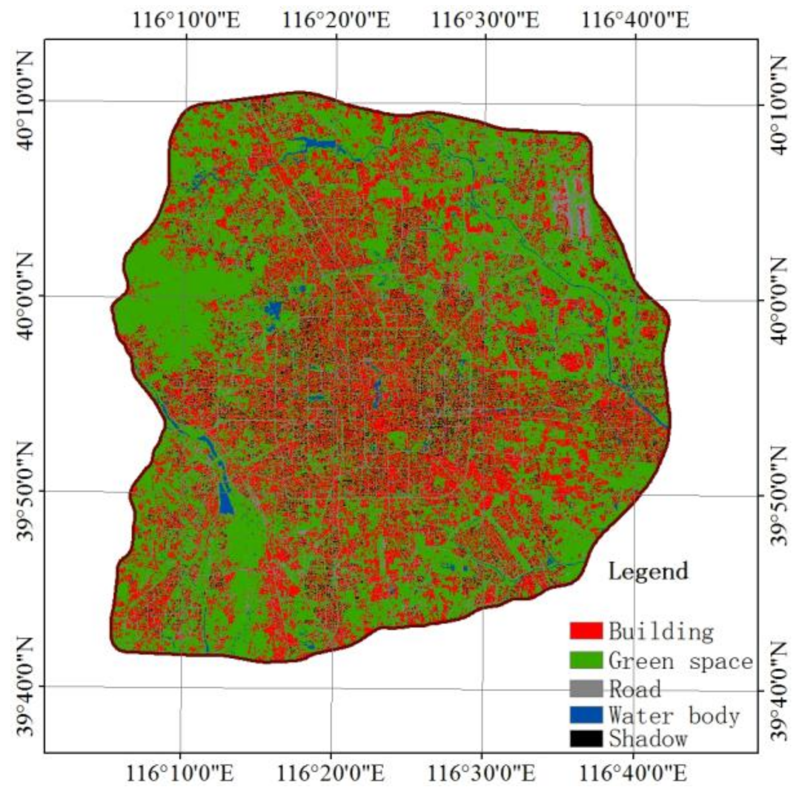
The support vector machine (SVM) algorithm was used to interpret the land cover of the study area based on GF-2 remote-sensing data [37]. First, we segmented the GF-2 remote-sensing image into image objects based on upon several adjustable criteria of homogeneity or heterogeneity in color and shape. Second, we acquired the good SVM model by training sample data and applied the model to classify the whole remote-sensing image in the study area. Finally, we manually modified the misclassification patches so as to improve the classification accuracy. We grouped the land cover into five classes: buildings, roads, green spaces, water bodies, and shadows. Buildings refer to building masses in residential areas, industrial areas, commercial areas, and public utilities. Roads refer to the main trunk roads that are identifiable in remote-sensing images. Green spaces refer to vegetation covers, including grasslands, and woodlands. Water bodies include waterways, ponds, reservoirs, and lakes. Shadows refer to the shadows of buildings with substantial elevations. One thousand random sample points were used to evaluate the land cover classification accuracy based on the confusion matrix [38]. The assessment results are shown in Table 1. Overall accuracy is over 90%, and the kappa coefficient is 87.83%. This high accuracy is able to satisfy the practical requirements of the study.
A land cover classification map of the study area is shown in Figure 3. The total area of Beijing within the 6th Ring Road is 2268.72 km2. The areas of buildings, roads, water bodies, shadows, and green spaces are 665.26, 261.13, 45.71, 90.57, and 1206.05 km2, respectively. Green spaces have the largest contribution, making up more than half of the total area of Beijing. Water bodies make the smallest contribution at 2%.
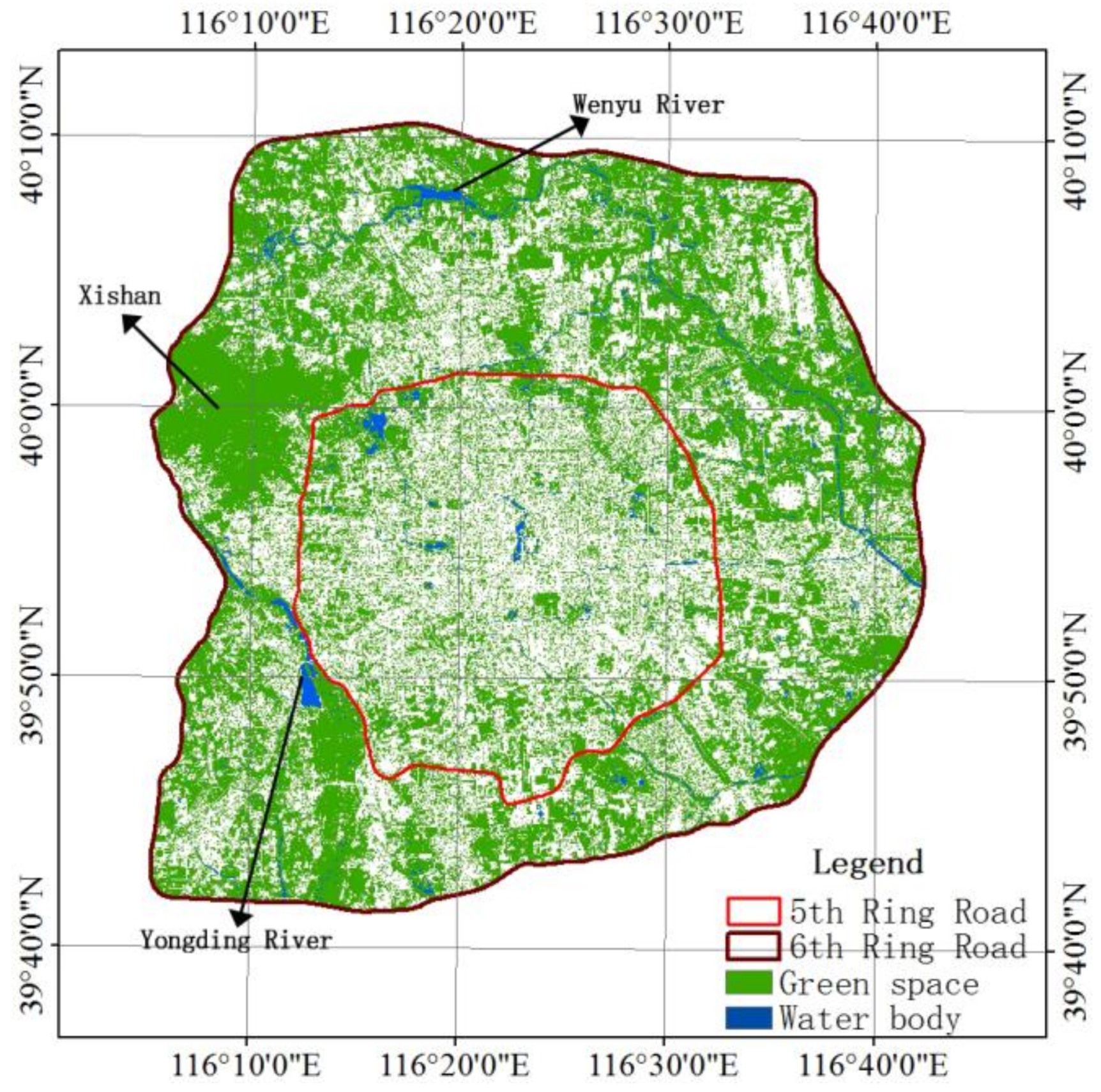
Green spaces and water bodies constitute medians that separate the main urban area of Beijing from the surrounding rural areas (Figure 4). Parks and green spaces near the 5th Ring Road form the first green median of Beijing. The northwest-trending Wenyu River in the north, the Xishan green space in the west, the Yongding River in the southeast, and the rural cultivated lands in the south form the second median of Beijing.
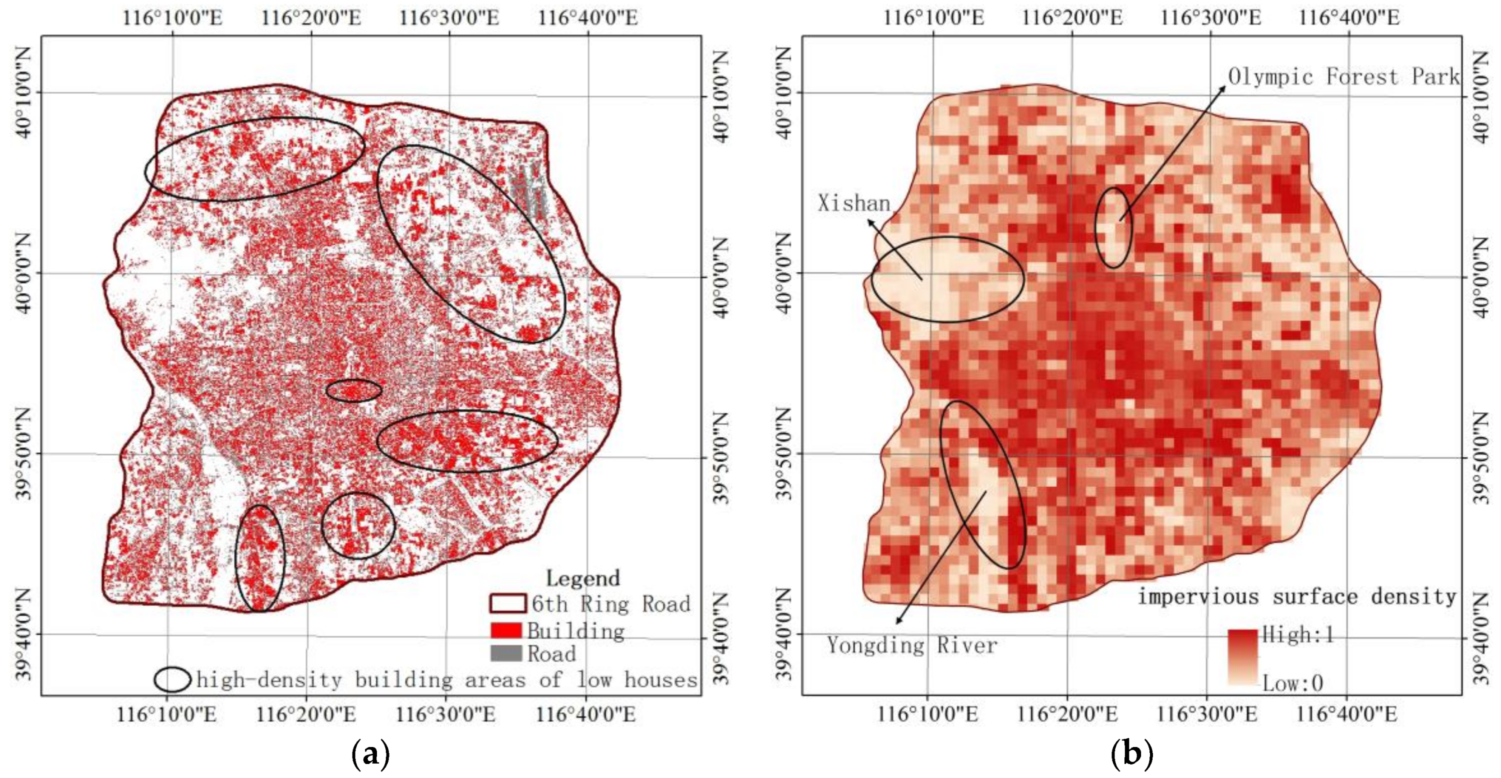
Buildings and roads make up the impervious surfaces of Beijing, and they collectively contribute 41% of its total area. Figure 5a shows the spatial distribution of the buildings and roads in Beijing. Additionally, Figure 5a shows that the buildings in Beijing are spatially distributed in two forms. The first form includes unit neighborhoods of unit building masses with substantial elevations and spacings. The second form includes high-density building areas of continuous low houses. Unit neighborhoods are the main form of building areas in Beijing. The high-density building areas of low houses are mostly scattered between the 5th and 6th Ring Road circles. In addition, there exist high-density building areas of low houses in the downtown areas of Da Zhalan, Qianmen, and Donghuashi. Figure 5b shows the impervious surface densities of Beijing featuring high densities in the downtown areas and low densities in the outskirts. The Xishan Mountains, Yongding River Basin, Summer Palace, Yuanmingyuan, and Olympic Forest Park scenic area have the lowest building densities. The northeast and southeast parts of Beijing, which comprise continuous villages and vast cultivated lands, also have low building densities.

2.3. Methods

2.3.1. Defining a New Measurement Unit

In this paper, we propose a novel spatial search method to extract the urban built-up area based on the spatial scale effect. The density of the impervious surfaces is used as the indicator to extract urban built-up area. Previous studies generally employed quadrilaterals as the basic measurement unit of calculating the impervious surface density. Geometrically, the spatial units in a quadrilateral grid are not only edge-neighbored (Figure 6a), but also corner-neighbored (Figure 6b). The statistical units in Figure 6b have only one common end vertex, and the spatial continuity between the statistical units is low, while those in a hexagonal grid are all edge-neighbored (Figure 6c). Hence, the graphic geometry implies that hexagons have better spatial scalability than quadrilaterals. In this study, hexagons were used as the basic spatial units for searching the continuous impervious surfaces.

2.3.2. Algorithm for Classifying Impervious Surface Densities

In this paper, we used the Jenks natural breaks algorithm to classify the value of impervious surfaces densities into two groups: a low-density group and a high-density group. The Jenks natural breaks algorithm identifies class intervals according to the natural grouping inherent to the data [39]. This method yields the best local grouping of like values and sets a classification boundary at points with high value divergences to achieve the maximum variance between classes and minimum variance within classes. The Jenks natural breaks algorithm minimizes the cost function J, defined in Equation (1):
J = 1 i n 1 < j < k d i s t ( d i , c j ) 1 j ( k 1 ) d i s t ( c j + 1 , c j )
where n is the data size of number of data points, k is the number of clusters and d i s t ( c j + 1 , c j ) computes the Euclidean distance between point d i and its closest cluster center c j . The d i s t ( c j + 1 , c j ) computes the Euclidean distance between cluster centers c j and c j + 1 . Equation (1) shows that the Jenks natural breaks algorithm not only searches for the minimum distance between data points and centers of clusters they belong to, but for the maximum difference between the cluster centers themselves [40].

2.3.3. Steps for Extracting Continuous Impervious Surfaces of High Density

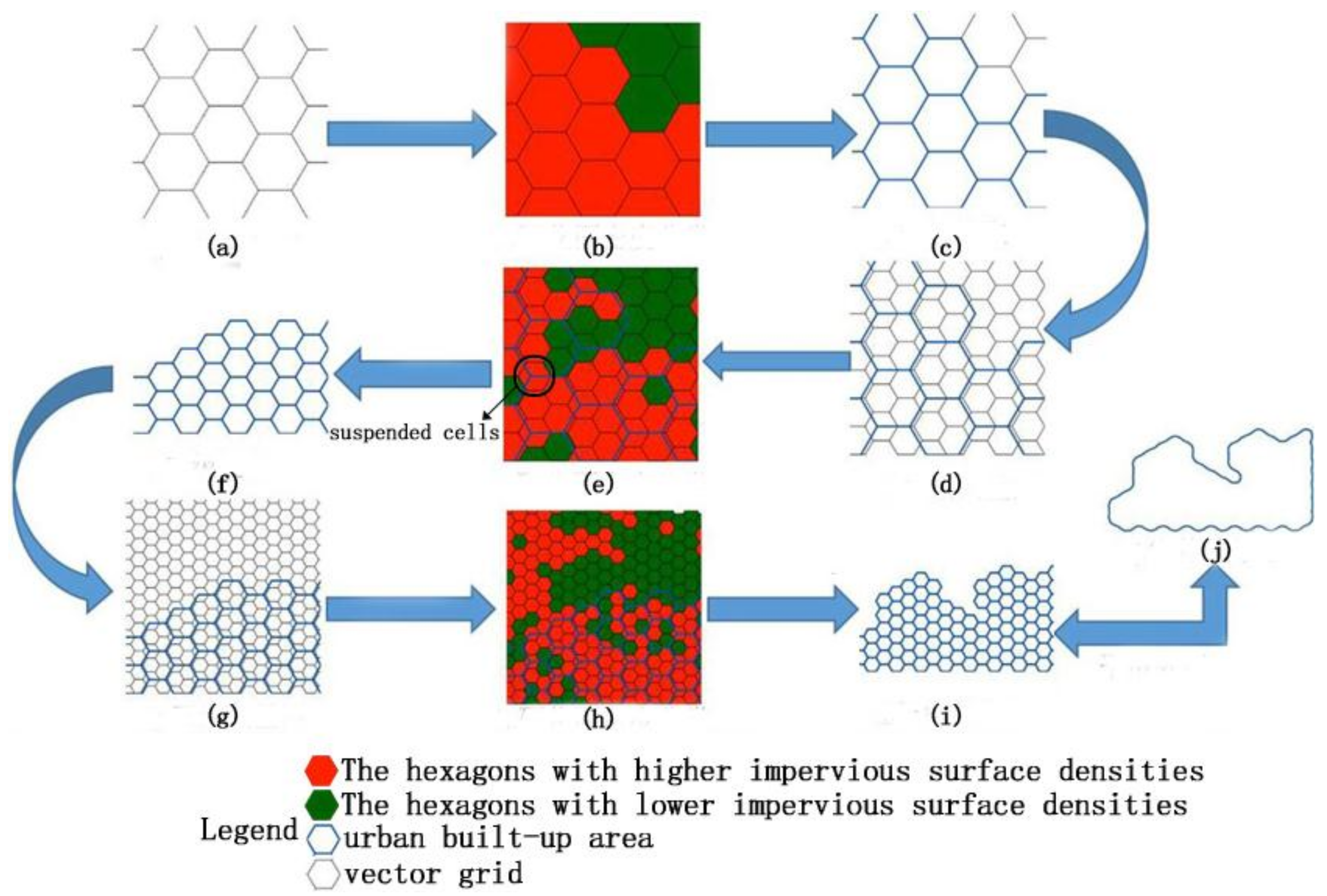
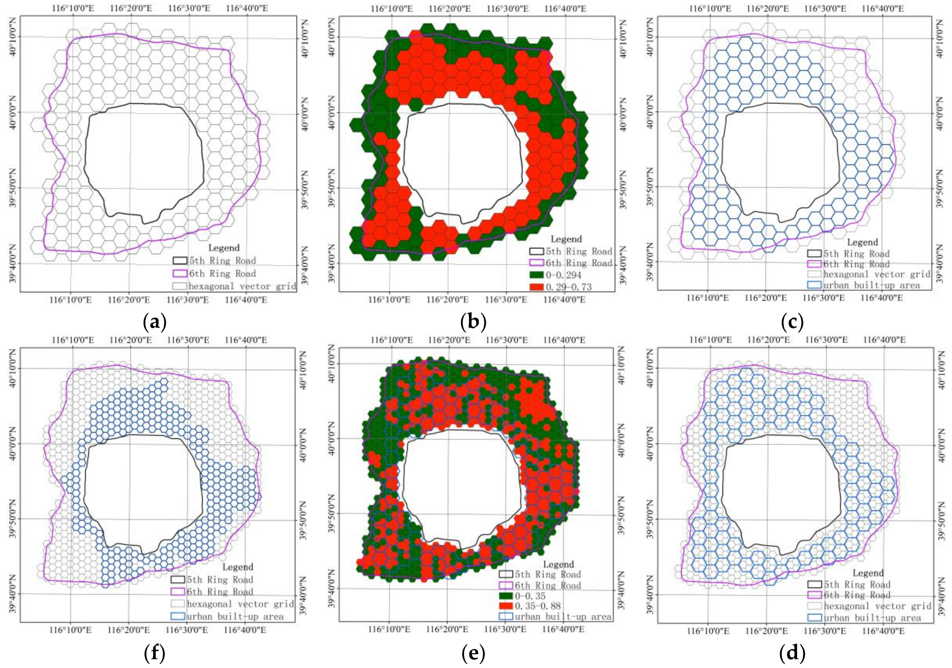
Previous studies frequently used inside-out strategies to extract the urban built-up area boundaries. In our study, we adopt an outside-in strategy to extract the urban built-up area boundaries. In the first step, we generated a number of different levels of edge-multiplied hexagonal vector grids according to the length of the urban streets. In terms of spatial morphology, the urban built-up area typically comprises neighborhood units segmented by streets. Hence, we use the length of urban streets as a basis to set the scales of hexagonal vector grids. A hexagonal grid at the smallest spatial scale should cover an integrated urban neighborhood. In the second step, we calculated the impervious surface densities using the hexagonal vector grid with the longest edge (Figure 7a). The impervious surfaces densities were automatically grouped into two classes using the Jenks natural breaks algorithm (Figure 7b). The edge hexagons with lower impervious surface densities and suspended hexagonal cells with higher impervious surface densities on the edge were deleted. The remaining hexagons with higher impervious surface densities were used as the extracted urban built-up area of the first level (Figure 7c). In the third step, based on the urban built-up area extracted from the first level (Figure 7d), we identified the hexagons with higher impervious surface densities from the second-level vector grid using the Jenks natural breaks algorithm (Figure 7e). In Figure 7e, we deleted the edge hexagons with lower impervious surface densities and the suspended hexagonal cells with higher impervious surface densities on the edge. The remaining hexagons with higher impervious surface densities were used as the urban built-up area extracted on the secondary level (Figure 7f). In the same manner, we gradually reduced the spatial scale of the hexagonal vector grid and extracted the continuous impervious surfaces of higher density at different scales. Eventually, we obtained the continuous impervious surface of higher densities at the smallest scale (Figure 7i). As the edge of a hexagonal vector grid is indented, we used the smooth line of ArcGIS 10.3 (Environmental Systems Research Institute: Redlands, CA, USA, 2013) to smooth the edge, and obtained a smooth urban built-up area boundary (Figure 7j).

2.3.4. Plausibility Check and Accuracy Assessment

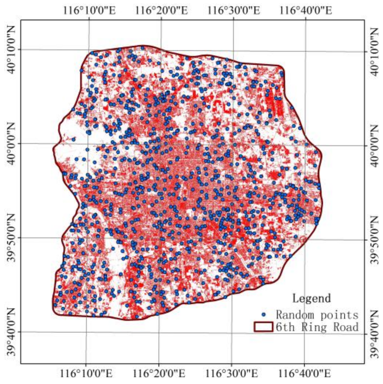
To quantitatively verify the rationale of the result, we first make the plausibility check based on nighttime light data. The values of nighttime light data in urban built-up area are always higher than those in rural areas. We present the statistics information of nighttime light data for inner part and outer part of the extracted Beijing built-up area boundary in boxplots and compare the distribution difference of nighttime light data [41]. Since rural landscapes are blended with urban landscapes at the rural-urban fringe, rural settlements are easily misclassified as urban impervious surfaces. We classified the impervious surfaces into two groups: rural settlements and urban built-up area. Then, we acquired 1000 real sample points from Google Maps, which belong to impervious surfaces (Figure 8). We used the sample points to assess the accuracy of the extracted Beijing built-up area based on the confusion matrix [38].

3. Results

Our measurements revealed that shorter streets in Beijing are approximately 300 m long, whereas longer streets are approximately 1500 m long. As the spatial resolution of the remote-sensing images used herein was 0.8 m, hexagonal vector grids with 240, 480, 960, and 1920 m edges were generated as the spatial unit system for extracting the urban built-up area of Beijing, using 240 m as the minimum scale. As the area within the 5th Ring Road is generally regarded as the urban built-up area of Beijing, the urban built-up area within the 5th and 6th Ring Roads was first extracted and then combined with the urban built-up area within the 5th Ring Road.
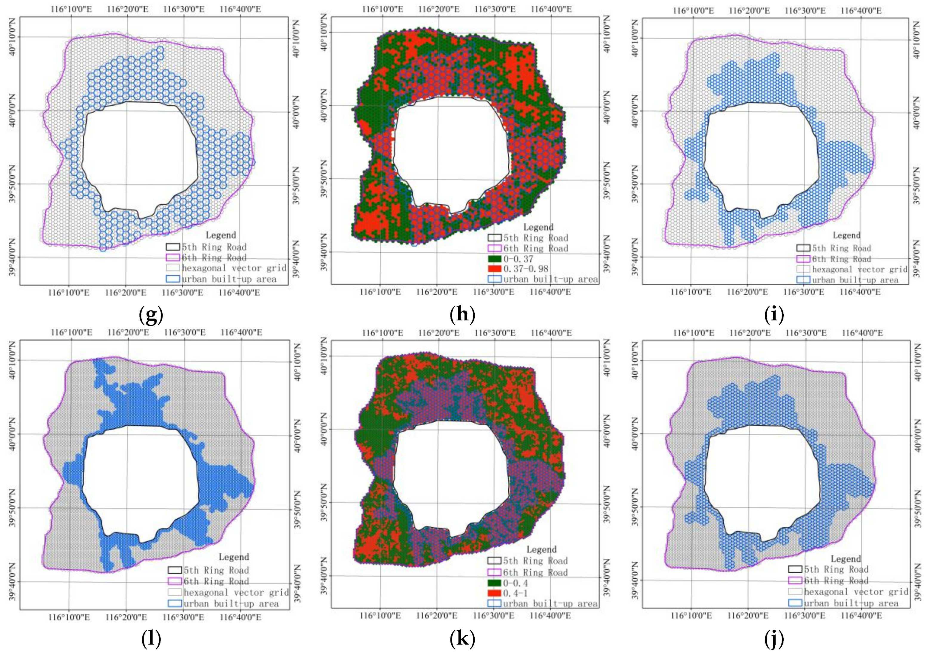
A hexagonal vector grid with a 1920 m edge was generated for the area between the 5th and 6th Ring Roads of Beijing (Figure 9a). The impervious surface density within each hexagonal cell was calculated using the zonal statistics module of ArcGIS 10.3. The resultant impervious surface densities were then grouped into two classes using Jenks natural breaks algorithm. The regions with impervious surface densities lower than 0.294 were defined as low-value regions, whereas those with densities exceeding or equal to 0.294 were defined as high-value regions (Figure 9b). Without affecting the continuity and closeness of the hexagonal vector grid, the low-value and suspended hexagonal cells on the edge were deleted. Consequently, the urban built-up area on the 1920 m scale was obtained (Figure 9c). In the same manner, the urban built-up area at the 960 m scale was extracted (Figure 9f) based on the urban built-up area boundary shown in Figure 9d. The threshold value for discriminating the impervious surface densities was 0.353 at the 960 m scale. The above-mentioned steps were repeated to extract the urban built-up areas of Beijing at 480 and 240 m scales (Figure 9i,l). The thresholds used for classifying impervious surface densities by the Jenks natural breaks algorithm were 0.374 and 0.4, respectively.
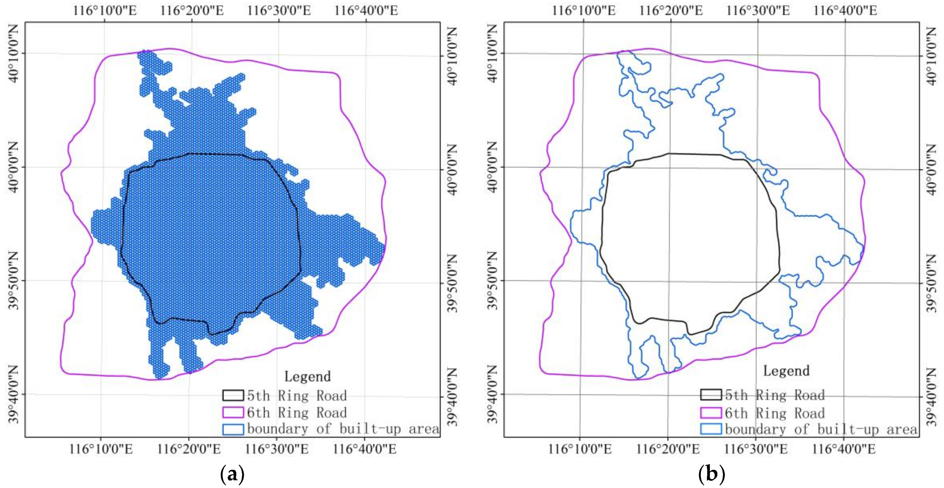
The urban built-up area extracted at the 240 m scale was combined with the hexagonal vector grid at the same scale to generate the Beijing built-up area within the 6th Ring Road. The hexagonal cells of the urban built-up area within the 6th Ring Road were fused (Figure 10a). The edges of the hexagonal vector grids were smoothed to obtain the eventual Beijing built-up area boundary (Figure 10b).
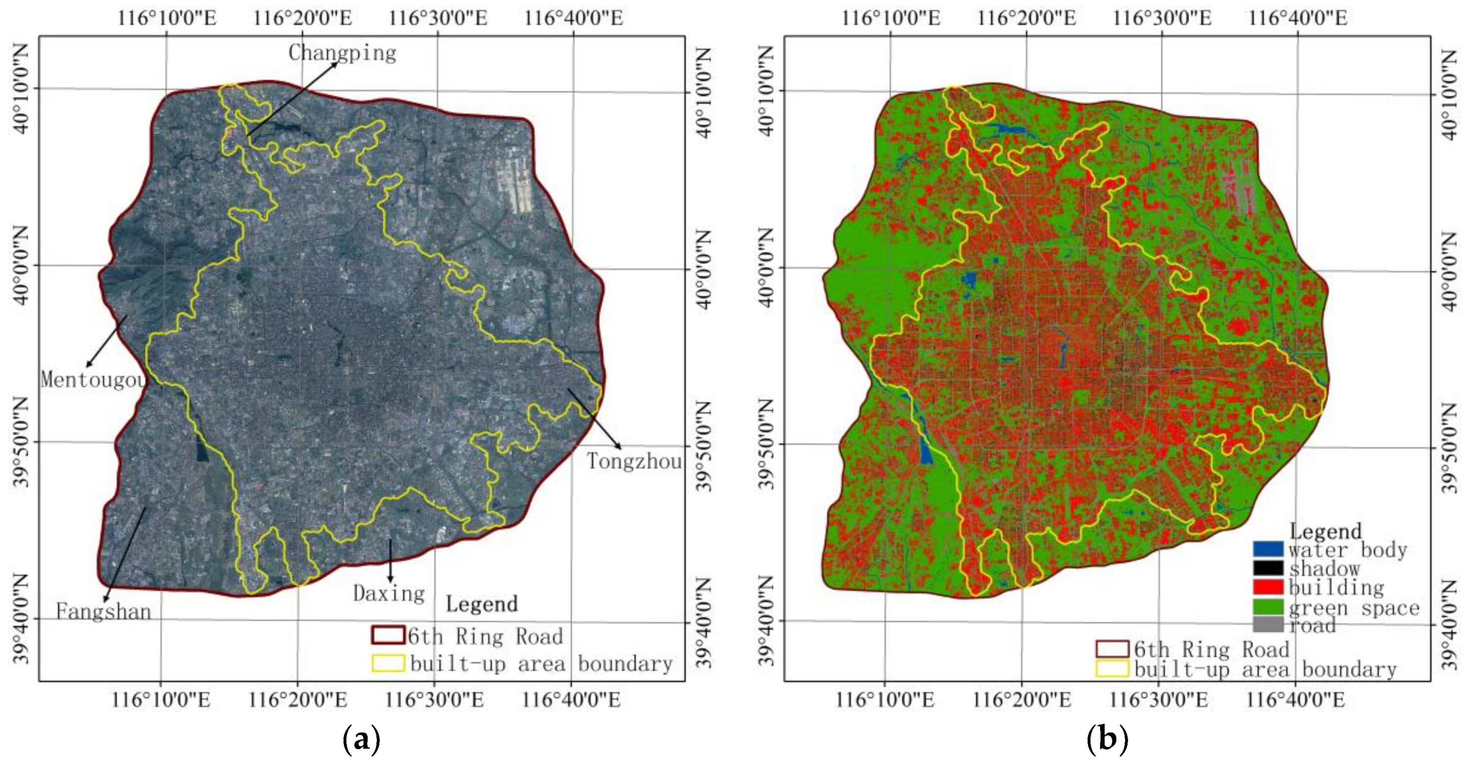
The resultant urban built-up area of Beijing is 1135.63 km2, which is 50% of the area of Beijing within the 6th Ring Road. The extracted urban built-up area boundary of Beijing was overlaid to the original remote-sensing images (Figure 11a) and to the land cover classification map of the area within the 6th Ring Road (Figure 11b). Overall, the extracted urban built-up area boundary of Beijing covered the relatively continuous impervious surfaces within the 6th Ring Road of Beijing. There are continuous green spaces and scattered rural settlements of low houses in the south and southeast parts and along the Wenyu River in the northeast of Beijing within the 6th Ring Road. These spaces and settlements do not belong to the urban built-up area in terms of landscape composition. The area to the northwest, the Xishan Mountains, and the vast villages to the north of the Xishan Mountains within the 6th Ring Road also do not belong to the urban built-up area of Beijing. The area to the southwest, the Yongding River, and the green median along the river within the 6th Ring Road separate the Fangshan District and Mentougou District from the urban built-up area of Beijing. In terms of urban expansion, Beijing has extended northwestward into the Changping District along the Beijing–Tibet Freeway, Beijing–Xinjiang High-Speed Railway, and Metro Line 15; northward along the Metro Line 5 and Provincial Highway S213; eastward into the Tongzhou District from the 5th Ring Road along the Metro Line Ba-Tong; and southward into the Daxing District along the southern 5th Ring Road, Luqiu Road, Metro Line Daxing, Metro Line Yizhuang, and Beijing–Shanghai Freeway. The extracted urban built-up area covered these areas and highlighted the prevailing orientation of the urban expansion of Beijing.

4. Discussion and Conclusions

4.1. Comparison with Previous Studies

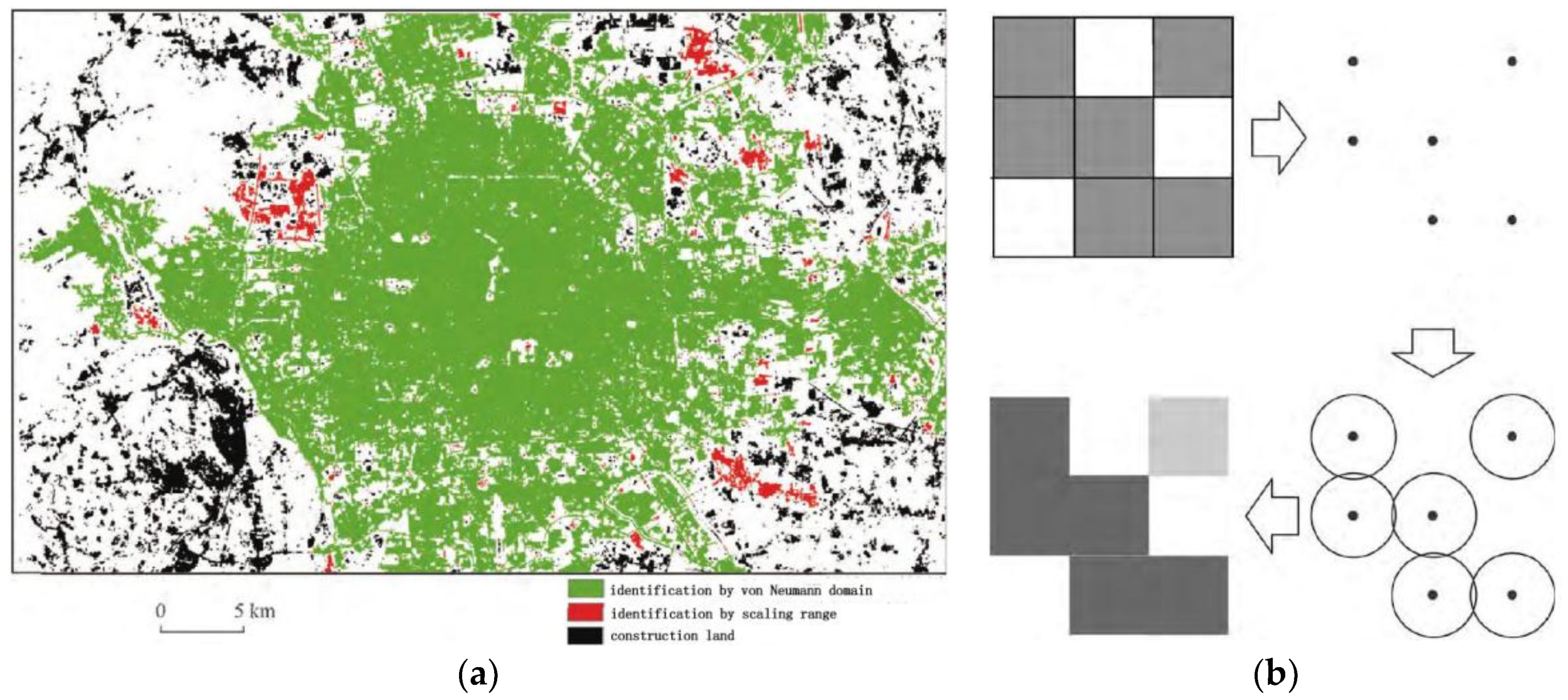
We compare our research with two previous studies in the same study area. Figure 12a shows the Beijing built-up area boundary extracted via neighborhood dilation, which was conducted by Tan et al. (2015) [28]. The basic principle of neighborhood dilation is illustrated in Figure 12b. First, the raster data center point of the construction land was extracted. Then, circular search units were generated with this center point, after which the pixels of the construction land intersected by the circular search units were fused to form the urban built-up area. The radii of the circular search units were determined according to the number of pixels of the construction land clustered in the search region as a function of the radii. Hence, when using this method, instead of being an independent exogenous variable, the radii of the circular search units are endogenous to the number of pixels of the built-up area clustered in the search region. In our study, different scales of hexagons were used as the search unit. The thresholds for discriminating impervious surface densities were automatically obtained using the Jenks natural breaks algorithm. This guarantees the exogeneity of the search unit scaling and avoids the subjectivity of manually defining single-scale search units and thresholds.
In addition, the method of neighborhood dilation failed to extract the continuous boundary of Beijing built-up area. The water bodies and some parks and green spaces within the territory of Beijing were not extracted, though they obviously belong to the urban built-up area of Beijing. In Figure 12a, the red region in the northeast, which lies to the north or on the Wenyu River and has been separated from the main urban area of Beijing by the Wenyu River and the surrounding green spaces, should not be included in the urban built-up area of Beijing. In our study, the impervious surfaces of lower densities were continuously removed in an outside-in manner. This guaranteed the internal spatial continuity of the extracted urban built-up area and enabled us to extract the continuous urban built-up area boundary. In addition, as descending search unit scales were used, the extracted urban built-up area contains the impervious surfaces with relatively higher densities.
Figure 13a shows the Beijing built-up area boundary extracted by Xu et al. (2016) [1]. The basic principle of this method is illustrated in Figure 13b,c. Kernel density interpolation was performed using the given bandwidth with the POI data. The contour line was extracted from the resultant kernel density distribution map. The area encircled by the contour line at each kernel density was calculated, and the mutation point of increase in area as a function of kernel density was used as the criterion for identifying the urban built-up area. In the research method, the POI is intended for use in navigation. Its spatial presentation characterizes the dense distribution along streets and the sparse distribution in urban neighborhoods and suburban regions. Hence, there can be more than one mutation point of area increase as a function of kernel density both within, and on, the boundary of Beijing. Determining an appropriate mutation point to be used as the criterion for identifying urban built-up area boundaries is still a debated topic. The kernel density distribution map generated by POI interpolation is more focused on the intensity level of economic activities and does not address the spatial continuity of urban impervious surfaces. Additionally, the bandwidth used for kernel density interpolation was merely an empirical value that lacks theoretical support. The boundary of the built-up area of Beijing extracted using this method was considerably rough. Further, no comparison was made in the study with the actual urban landscapes of Beijing. In our study, the urban built-up area boundary of Beijing was extracted from high-spatial-resolution remote-sensing images. This helped us in visualizing the extraction process and made the result more direct.

4.2. Plausibility Check and Accuracy Assesement

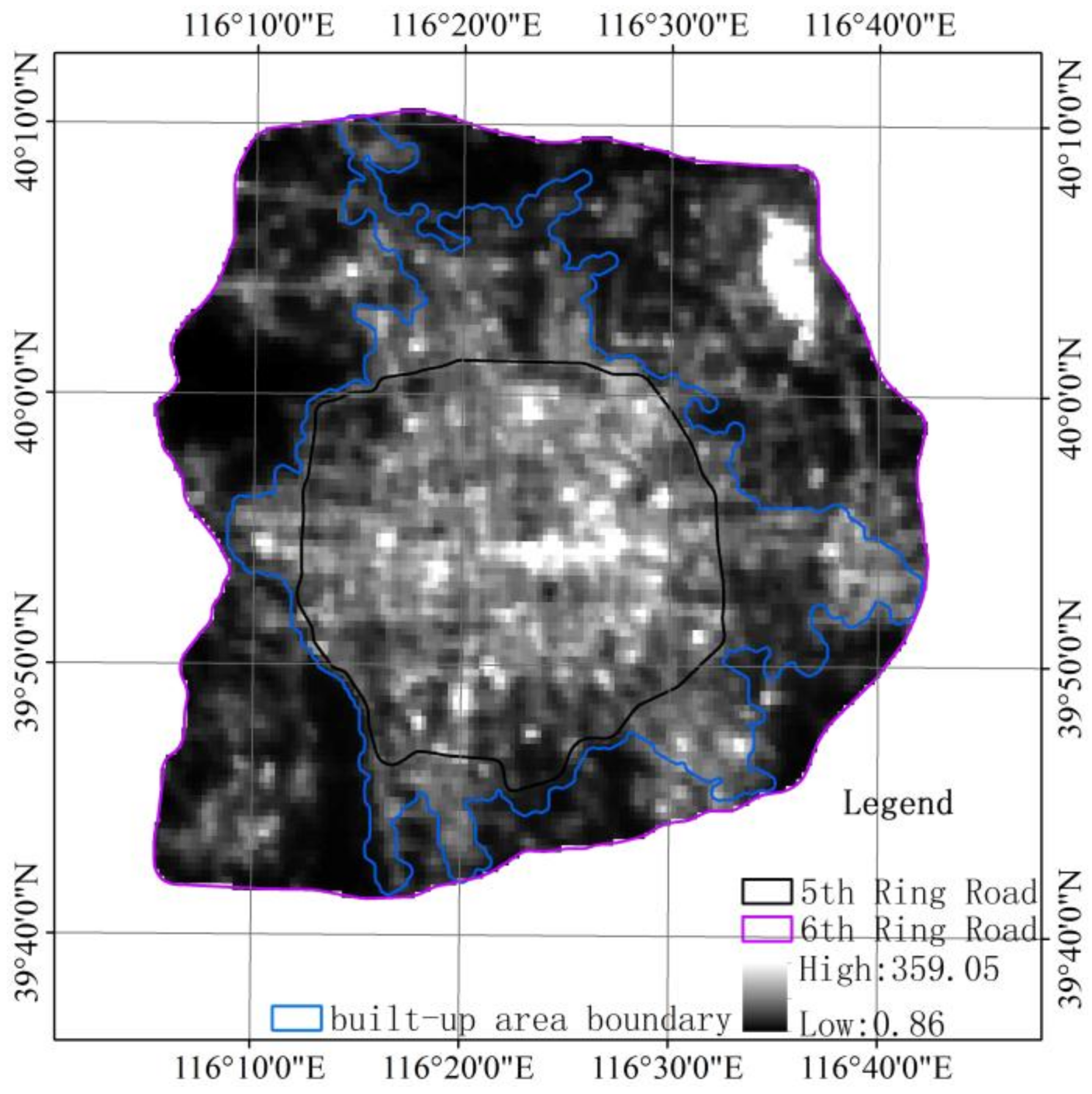
The extracted Beijing built-up area boundary was overlaid on the nighttime light map of Beijing within the 6th Ring Road (Figure 14). It was found that the extracted Beijing built-up area concurred with the high-value continuous grids of the nighttime light image. The Beijing built-up area boundary highlighted the prevailing orientation of the urban expansion of Beijing toward the north, south, and east. Unfortunately, nighttime light is divergent, and the spatial resolution of the nighttime light data is low. Hence, no obvious differences in value were observed in the nighttime light data at the urban-rural junctions.
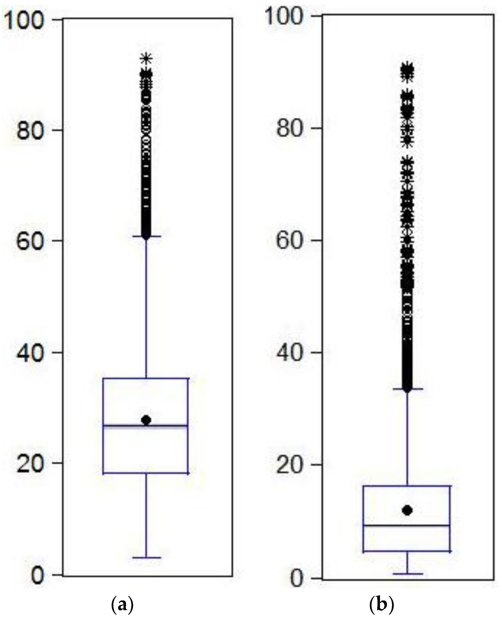
To quantitatively verify the rationale of the result, we present the statistics information of nighttime light data for inner part and outer part of the extracted Beijing built-up area boundary in boxplots (Figure 15). In Figure 15a, the lower quartile is 18.36, the median value is 26.88, and the upper quartile is 35.5. In Figure 15b, the lower quartile is 4.9, the median value is 9.46, and the upper quartile is 16.96. It is obvious that the inner part of the extracted Beijing built-up area boundary contains the most grid units of high-value nighttime light data. To some degree, this indicates that the extracted urban built-up area is plausible.
The accuracy assessment of the extracted Beijing built-up area based on 1000 real sample points is shown in Table 2. The overall accuracy is 94.1%, and the kappa coefficient is 87.69%. Some rural settlements were misclassified as urban built-up areas at the rural-urban fringe due to the higher impervious surface densities. In fact, it is impossible to entirely distinguish the rural settlements from urban built-up areas, because the rural landscapes are blended with urban landscapes at the rural-urban fringe. The result of accuracy assessment indicates that we have acquired a relatively objective Beijing built-up area boundary.

4.3. The Measurement Scale Effects on the Results

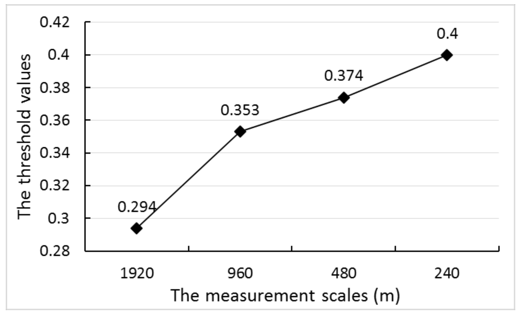
Figure 16 shows the tendency of the threshold values for discriminating the impervious surface densities with the spatial scales in the process of extracting Beijing built-up area. It is obvious that the threshold values increase with the increase of measurement scales of the hexagonal vector grids. This means that we acquired much higher-density impervious surfaces by decreasing the measurement scales.
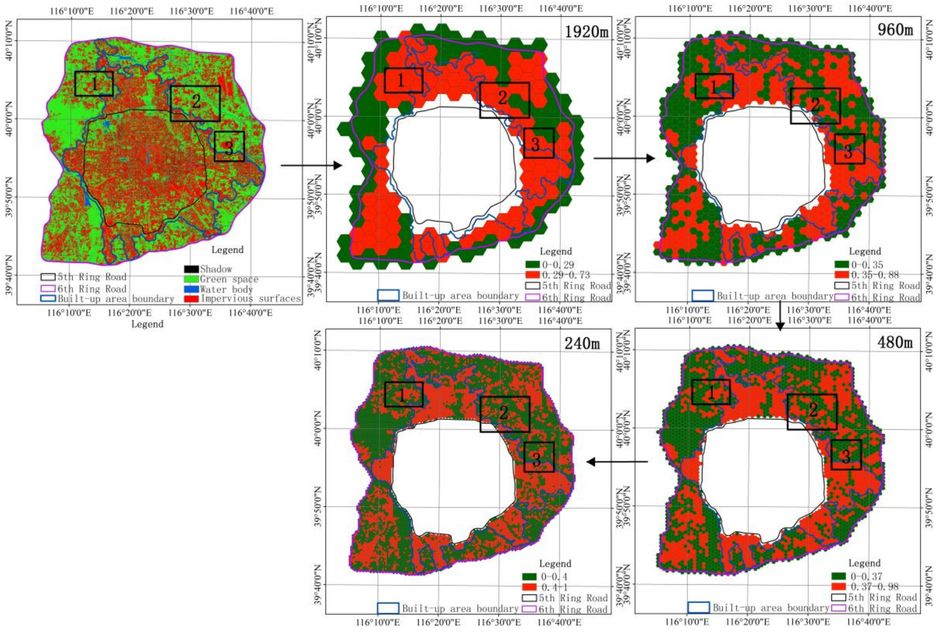
To visualize the measurement scale effects on the extracted Beijing built-up area, we choose three typical subregions on the edge of the extracted built-up area boundary (Figure 17). The three subregions belong to the rural-urban fringe, and the rural settlements are presented as small clusters scattered across the rural green space landscapes. Rural landscapes are blended with urban landscapes within the three subregions. At the measurement scale of 1920 m, the impervious surface densities in the three subregions are higher than 0.29 and these areas were classified as built-up areas at this scale. When we measured the impervious surface densities with 960 m hexagonal vector grids, the threshold value for discriminating impervious densities increased to 0.35 by the Jenks natural breaks algorithm. However, the hexagonal vector grids with higher impervious surface densities are discontinuous within the three subregions. The rural settlements with higher impervious surface densities were identified and were separated from the continuous high-density impervious surfaces by rural green space landscapes. When the measurement scales decreased to 480 m and 240 m, the threshold values for discriminating impervious surfaces increased to 0.37 and 0.4, respectively, and the hexagonal vector grids containing rural settlements were identified gradually. At the measurement scale of 240 m, the higher densities’ continuous impervious surfaces were extracted as the Beijing built-up area.

5. Conclusions

In this paper, a novel method of extracting the urban built-up area boundary in an outside-in manner with different scales of hexagonal vector grids was proposed based on the scale effect. Compared with commonly-used spatial search algorithms, our method uses different scales of hexagons as the search unit. This guarantees the exogeneity of the search unit scaling and avoids the subjectivity of manually defining single-scale search units. Compared with the methods of a threshold indicator, our method automatically obtains the thresholds using the Jenks natural breaks algorithm at different spatial scales. Hence, our method is appropriate for extracting urban built-up area. The proposed method was applied to extract the urban built-up area boundary of Beijing with high-spatial-resolution remote-sensing images as the base data for visualizing the extraction process. The extracted urban built-up area of Beijing contains the continuous impervious surface of high densities. The Beijing built-up area boundary can be directly presented in the concrete geographic space and directly shows the skyline of the built-up area and the prevailing orientation of urban expansion. The extracted Beijing built-up area boundary can serve as a reference in decision-making for space planning and land-use control of Beijing.

Acknowledgments

This research was financially supported by the National Key R & D Program of China (grant No. 2017YFB0503805) and the Special Project on High Resolution of Earth Observation System for Major Function Oriented Zones Planning (grant No. 00-Y30B14-9001-14/16).

Author Contributions

Mingguang Tu conceived and designed the research; Yi Zhou and Shixin Wang contributed materials; and Mingguang Tu and Wenliang Liu wrote the paper.

Conflicts of Interest

The authors declare no conflict of interest.

References

  1. Xu, Z.; Gao, X. A novel method for identifying the boundary of urban built-up areas with poi data. Acta Geogr. Sin. 2016, 71, 928–939. [Google Scholar]
  2. Tannier, C.; Thomas, I.; Vuidel, G.; Frankhauser, P. A fractal approach to identifying urban boundaries. Geogr. Anal. 2011, 43, 211–227. [Google Scholar] [CrossRef]
  3. Forstall, R.L.; Chan, K.W. Urban places: Statistical definitions. Int. Encycl. Soc. Behav. Sci. 2015, 24, 854–861. [Google Scholar]
  4. Taubenböck, H.; Wiesner, M.; Felbier, A.; Marconcini, M.; Esch, T.; Dech, S. New dimensions of urban landscapes: The spatio-temporal evolution from a polynuclei area to a mega-region based on remote sensing data. Appl. Geogr. 2014, 47, 137–153. [Google Scholar] [CrossRef]
  5. Florida, R. Megaregions: The importance of place. Harv. Bus. Rev. 2008, 33, 18–19. [Google Scholar]
  6. Pryor, R.J. Defining the rural-urban fringe. Soc. Forces 1968, 47, 202–215. [Google Scholar] [CrossRef]
  7. Fesenmaier, D.R.; Goodchild, M.F.; Morrison, S. The spatial structure of the rural-urban fringe: A multivariate approach. Can. Geogr. 1979, 23, 255–265. [Google Scholar] [CrossRef]
  8. Sullivan, W.C.; Lovell, S.T. Improving the visual quality of commercial development at the rural-urban fringe. Landsc. Urban Plan. 2006, 77, 152–166. [Google Scholar] [CrossRef]
  9. Laurence, J.C.; Cui, G. Administrative changes and urban population in China. Ann. Assoc. Am. Geogr. 2015, 77, 373–395. [Google Scholar] [CrossRef]
  10. Martin, M.F. Defining China’s rural population. China Q. 1992, 130, 392–401. [Google Scholar] [CrossRef]
  11. Chan, K.W. Misconceptions and complexities in the study of China’s cities: Definitions, statistics, and implications. Eurasian Geogr. Econ. 2007, 48, 383–412. [Google Scholar] [CrossRef]
  12. Zhou, Y.S.Y. Toward establishing the concept of physical urban area in China. Acta Geogr. Sin. 1995, 62, 289–301. [Google Scholar]
  13. Mao, Q.; Ying, L.; Kang, W.; Qingfei, Z. Spatio-temporal changes of population density and urbanization pattern in China (2000–2010). China City Plan. Rev. 2016, 25, 8–14. [Google Scholar]
  14. Wang, F.; Zhou, Y. Modelling urban population densities in Beijing 1982–90: Suburbanisation and its causes. Urban Stud. 2014, 36, 271–287. [Google Scholar] [CrossRef]
  15. Luo, S.G.; Johnston, A.; Chen, D.C. Approach to delimiting metropolitan regions’ boundary and grading urban hierarchy within a metropolitan region—A case study of Shanghai metropolitan region. Chin. Geogr. Sci. 2008, 18, 197–205. [Google Scholar] [CrossRef]
  16. Clark, C. Urban population densities. J. R. Stat. Soc. 1951, 114, 490–496. [Google Scholar] [CrossRef]
  17. Masek, J.G.; Lindsay, F.E.; Goward, S.N. Dynamics of urban growth in the Washington DC metropolitan area, 1973–1996, from Landsat observations. Int. J. Remote Sens. 2000, 21, 3473–3486. [Google Scholar] [CrossRef]
  18. Hereher, M.E. Analysis of urban growth at Cairo, Egypt using remote sensing and GIS. Nat. Sci. 2012, 4, 355–361. [Google Scholar] [CrossRef]
  19. Abed, J.; Kaysi, I. Identifying urban boundaries: Application of remote sensing and geographic information system technologies. Can. J. Civ. Eng. 2003, 30, 992–999. [Google Scholar] [CrossRef]
  20. Li, Y.; Zhan, Q. Identification of urban boundaries based on geographic information system and land cover: A case in Wuhan. Urban. Land Use 2015, 2014, 63–70. [Google Scholar]
  21. Georg, I.; Blaschke, T.; Taubenböck, H. Are we in boswash yet? A multi-source geodata approach to spatially delimit urban corridors. ISPRS Int. Geo-Inf. 2018, 7, 15. [Google Scholar] [CrossRef]
  22. Taubenböck, H.; Ferstl, J.; Dech, S. Regions set in stone—Delimiting and categorizing regions in Europe by settlement patterns derived from EO-data. ISPRS Int. Geo-Inf. 2017, 6, 55. [Google Scholar] [CrossRef]
  23. Small, C.; Pozzi, F.; Elvidge, C.D. Spatial analysis of global urban extent from DMSP-OLS night lights. Remote Sens. Environ. 2005, 96, 277–291. [Google Scholar] [CrossRef]
  24. Liu, Z.F.; He, C.Y.; Zhang, Q.F.; Huang, Q.X.; Yang, Y. Extracting the dynamics of urban expansion in China using DMSP-OLS nighttime light data from 1992 to 2008. Landsc. Urban. Plan 2012, 106, 62–72. [Google Scholar] [CrossRef]
  25. Imhoff, M.L.; Lawrence, W.T.; Stutzer, D.C.; Elvidge, C.D. A technique for using composite DMSP/OLS “city lights” satellite data to map urban area. Remote Sens. Environ. 1997, 61, 361–370. [Google Scholar] [CrossRef]
  26. Rozenfeld, H.D.; Rybski, D.; Andrade, J.S.; Batty, M.; Stanley, H.E.; Makse, H.A. Laws of population growth. Proc. Natl. Acad. Sci. USA 2008, 105, 18702–18707. [Google Scholar] [CrossRef] [PubMed]
  27. Rozenfeld, H.D.; Rybski, D.; Gabaix, X.; Makse, H.A. The area and population of cities: New insights from a different perspective on cities. Am. Econ. Rev. 2011, 101, 2205–2225. [Google Scholar] [CrossRef]
  28. Tan, X.; Chen, Y. Urban boundary identification based on neighborhood dilation. Prog. Geogr. 2015, 34, 1259–1265. [Google Scholar]
  29. Zha, Y.; Gao, J.; Ni, S. Use of normalized difference built-up index in automatically mapping urban areas from tm imagery. Int. J. Remote Sens. 2003, 24, 583–594. [Google Scholar] [CrossRef]
  30. Pesaresi, M.; Gerhardinger, A.; Kayitakire, F. A robust built-up area presence index by anisotropic rotation-invariant textural measure. IEEE J. Stars 2008, 1, 180–192. [Google Scholar] [CrossRef]
  31. Su, F.Z.; Gao, Y.; Zhou, C.H.; Yang, X.M.; Fei, X.Y. Scale effects of the continental coastline of China. J. Geogr. Sci. 2011, 21, 1101–1111. [Google Scholar] [CrossRef]
  32. Yan, G.J.; Hu, R.H.; Wang, Y.T.; Ren, H.Z.; Song, W.J.; Qi, J.B.; Chen, L. Scale effect in indirect measurement of leaf area index. IEEE Trans. Geosci. Remote Sens. 2016, 54, 3475–3484. [Google Scholar] [CrossRef]
  33. Woodcock, C.E.; Strahler, A.H. The factor of scale in remote-sensing. Remote Sens. Environ. 1987, 21, 311–332. [Google Scholar] [CrossRef]
  34. Krehl, A.; Siedentop, S.; Taubenböck, H.; Wurm, M. A comprehensive view on urban spatial structure: Urban density patterns of German city regions. ISPRS Int. Geo-Inf. 2016, 5, 76. [Google Scholar] [CrossRef]
  35. Taubenböck, H.; Standfuß, I.; Klotz, M.; Wurm, M. The physical density of the city—Deconstruction of the delusive density measure with evidence from two European megacities. ISPRS Int. Geo-Inf. 2016, 5, 206. [Google Scholar] [CrossRef]
  36. Aiazzi, B.; Baronti, S.; Selva, M.; Alparone, L. Enhanced Gram-Schmidt Spectral Sharpening Based on Multivariate Regression of MS and Pan Data. In Proceedings of the IEEE International Conference on Geoscience and Remote Sensing Symposium, Denver, CO, USA, 31 July–4 August 2006; pp. 3806–3809. [Google Scholar]
  37. Serpico, S.B. Support vector machines for remote sensing image classification. Proc. SPIE 2001, 4170, 160–166. [Google Scholar]
  38. Ghani, N.L.A.; Abidin, S.Z.Z.; Khalid, N.E.A. Accuracy Assessment of Urban Growth Pattern Classification Methods Using Confusion Matrix and ROC Analysis. In Proceedings of the 1st International Conference on Soft Computing in Data Science, Putrajaya, Malaysia, 2–3 September 2015. [Google Scholar]
  39. North, M.A. A Method for Implementing a Statistically Significant Number of Data Classes in the Jenks Algorithm. In Proceedings of the International Conference on Fuzzy Systems and Knowledge Discovery, Tianjin, China, 14–16 August 2009; pp. 35–38. [Google Scholar]
  40. Khan, F. An initial seed selection algorithm for k-means clustering of georeferenced data to improve replicability of cluster assignments for mapping application. Appl. Soft Comput. 2012, 12, 3698–3700. [Google Scholar] [CrossRef]
  41. Iglewicz, B.; Hoaglin, D. Use of boxplots for process evaluation. J. Qual. Technol. 1987, 19, 180–190. [Google Scholar] [CrossRef]
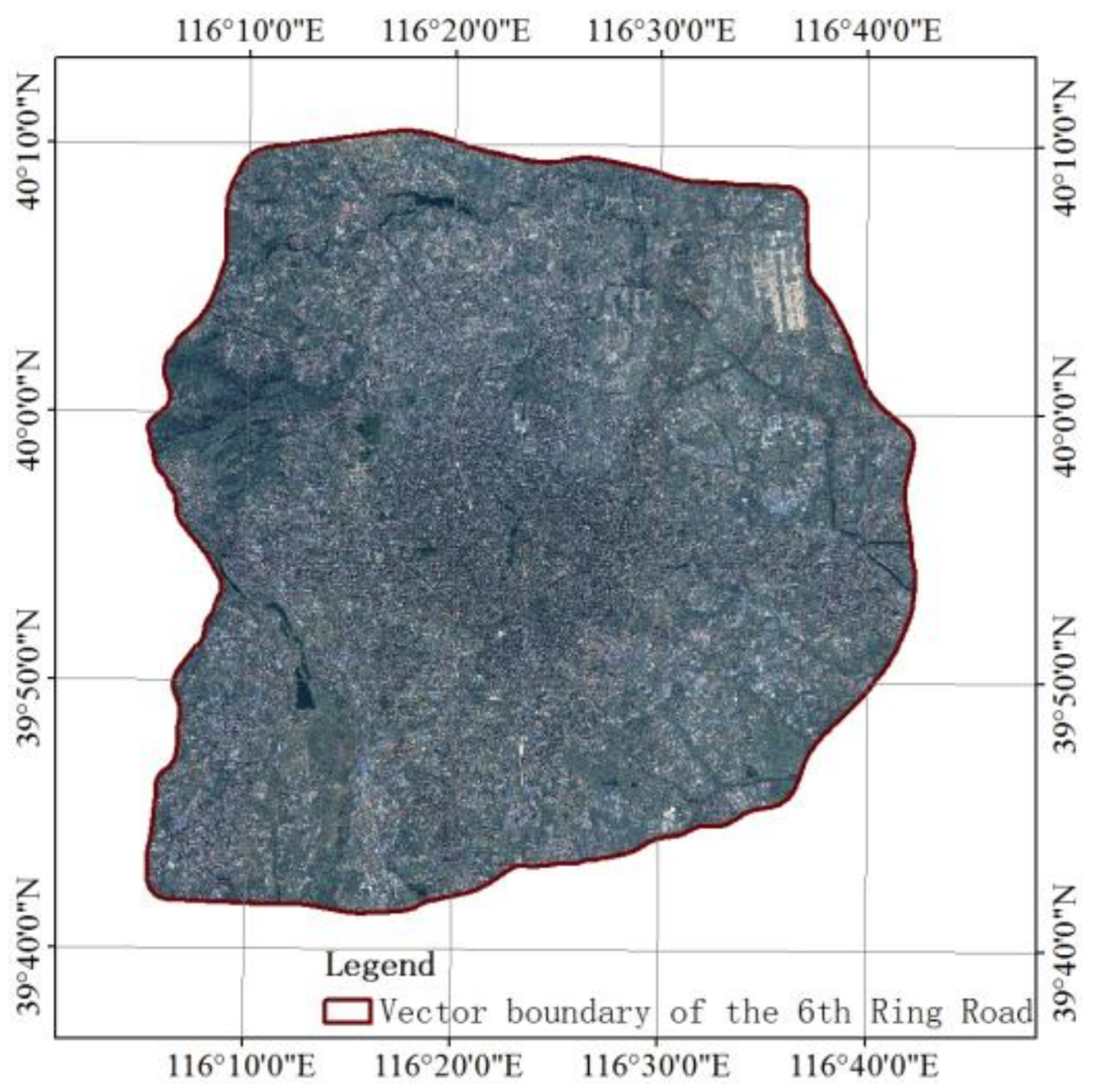
Figure 1. The study area and GF-2 image of Beijing within the 6th Ring Road.
Ijgi 07 00135 g001
Figure 2. The DMSP/OLS stable nighttime light data from 2015 in the study area.
Ijgi 07 00135 g002
Figure 3. Land cover classification of Beijing within the 6th Ring Road.
Ijgi 07 00135 g003
Figure 4. Distribution of green spaces and water bodies within the 6th Ring Road of Beijing.
Ijgi 07 00135 g004
Figure 5. (a) Distribution of buildings and roads within the 6th Ring Road; and (b) grid impervious surface density within the 6th Ring Road.
Ijgi 07 00135 g005
Figure 6. Spatial unit neighborhood of the quadrilateral and hexagonal grids: (a) edge-neighbored quadrilateral grids; (b) corner-neighbored quadrilateral grids; and (c) edge-neighbored hexagonal grids.
Ijgi 07 00135 g006
Figure 7. Flowchart of urban built-up area boundary extraction: (a) first-level vector grid; (b) impervious surface density classification in first-level vector grid; (c) first-level extraction; (d) second-level vector grid; (e) impervious surface density classification in second-level vector grid; (f) second-level extraction; (g) third-level vector grid; (h) impervious surface density classification in third-level vector grid; (i) third-level extraction; and (j) urban built-up area boundary smoothing.
Ijgi 07 00135 g007
Figure 8. One thousand real sample points used to assess the accuracy of the extracted Beijing built-up area.
Ijgi 07 00135 g008
Figure 9. Flowchart for extracting the Beijing built-up area boundary: (a) hexagonal vector grids with 1920 m edges; (b) impervious surface classification at the 1920 m scale; (c) extraction at the 1920 m scale; (d) hexagonal vector grids with 960 m edges; (e) impervious surface classification at the 960 m scale; (f) extraction at the 960 m scale; (g) hexagonal vector grids with 480 m edges; (h) impervious surface density classification at the 480 m scale; (i) extraction at the 480 m scale; (j) hexagonal vector grids with 240 m edges; (k) impervious surface density classification at the 240 m scale; and (l) extraction at the 240 m scale.
Ijgi 07 00135 g009aIjgi 07 00135 g009b
Figure 10. Post-treatment of the extracted urban built-up area boundary: (a) the hexagonal cells of the built-up area within the 6th Ring Road were fused; and (b) the smoothed urban built-up area of Beijing.
Ijgi 07 00135 g010
Figure 11. The Beijing built-up boundary: (a) overlaid on the original remote-sensing images; and (b) overlaid on the land cover classification map of the area within the 6th Ring Road.
Ijgi 07 00135 g011
Figure 12. (a) The Beijing built-up area boundary adapted from [28]; and (b) the basic principle of neighborhood dilation.
Ijgi 07 00135 g012
Figure 13. (a) Beijing built-up area boundary adapted from [1]; (b) kernel density interpolation and the contour line; and (c) the criterion for identifying the built-up area.
Ijgi 07 00135 g013
Figure 14. Plausibility check with nighttime light data.
Ijgi 07 00135 g014
Figure 15. The box plots of nighttime light data for: (a) the inner part and (b) the outer part of the extracted Beijing built-up area boundary.
Ijgi 07 00135 g015
Figure 16. The tendency of the threshold values with the measurement scales of the hexagonal vector grids.
Ijgi 07 00135 g016
Figure 17. Visualization of the measurement scale effects on extracting the urban built-up area.
Ijgi 07 00135 g017
Table 1. Accuracy assessment of land cover classification in the study areas.
ClassBuildingsRoadsGreen SpacesWater BodiesShadowsUser’s Accuracy
Buildings2071940488.46%
Roads1413130585.62%
Green spaces3829141191.80%
Water bodies00076692.68%
Shadows121920193.93%
Producer’s accuracy92%81.88%97.32%85.39%88.55%
Overall accuracy: 90.60%; kappa coefficient: 87.83%
Table 2. Accuracy assessment of the extracted Beijing built-up area.
ClassBuilt-Up AreaRural SettlementsUser’s Accuracy
Built-up area5723394.55%
rural settlements2636993.42%
Producer’s accuracy95.65%91.79%
Overall accuracy: 94.1%; kappa coefficient: 87.69%