Generative Street Addresses from Satellite Imagery

 ,
,
Abstract
:1. Introduction
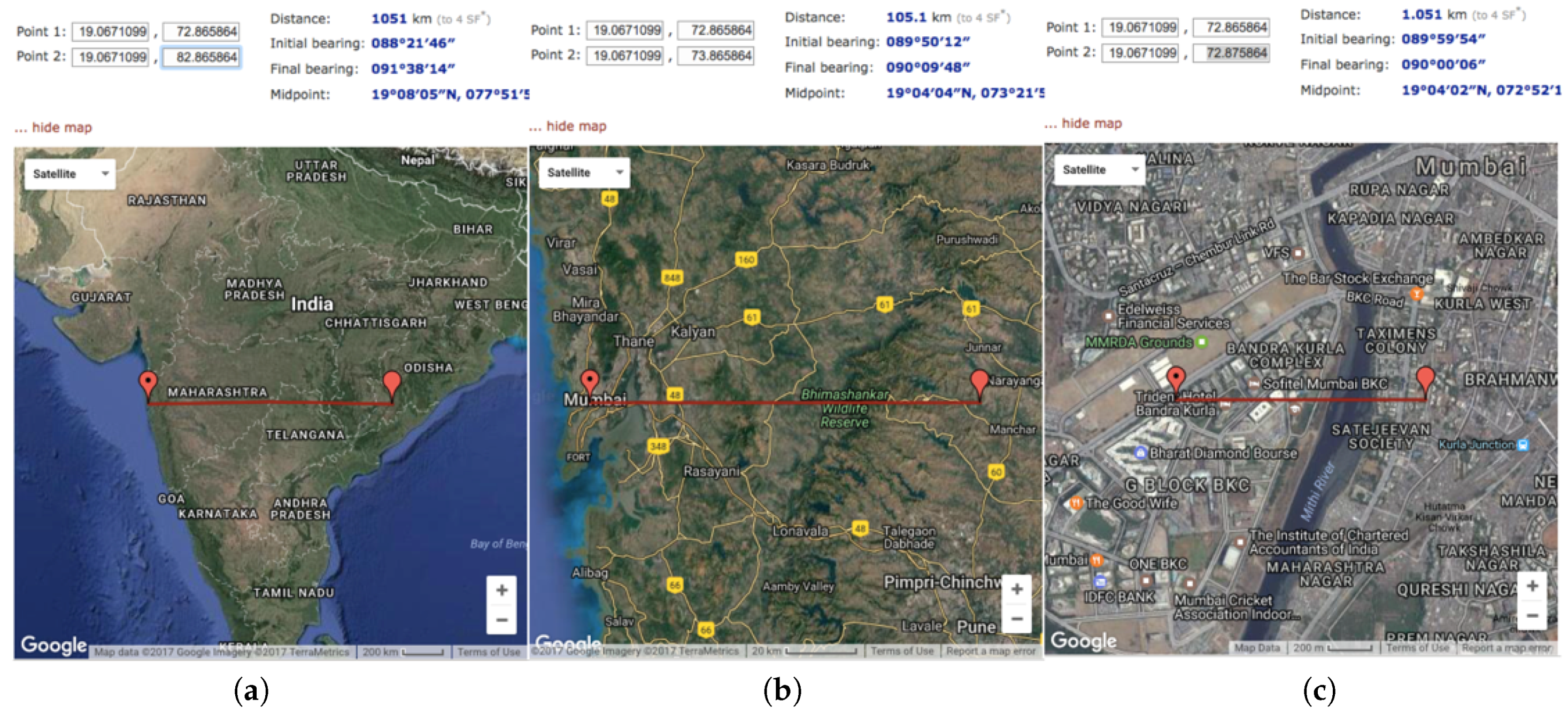
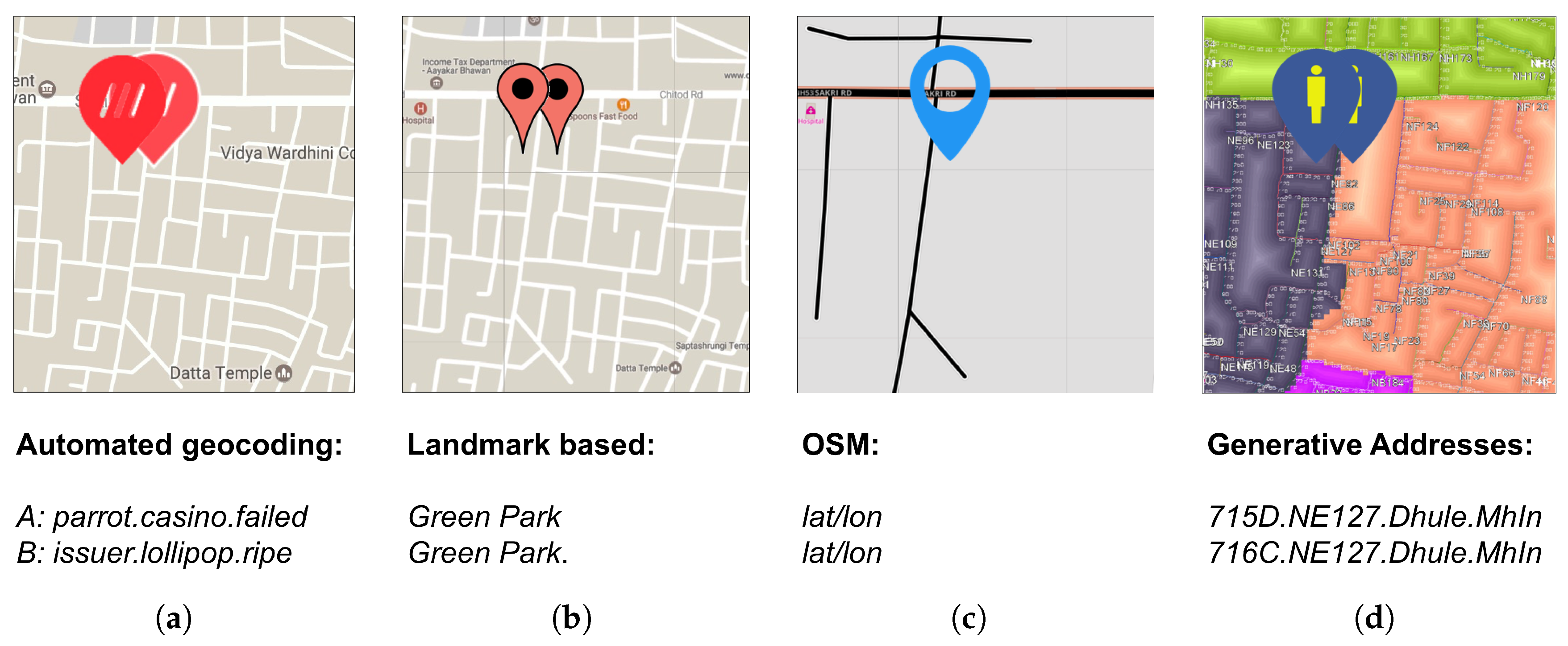
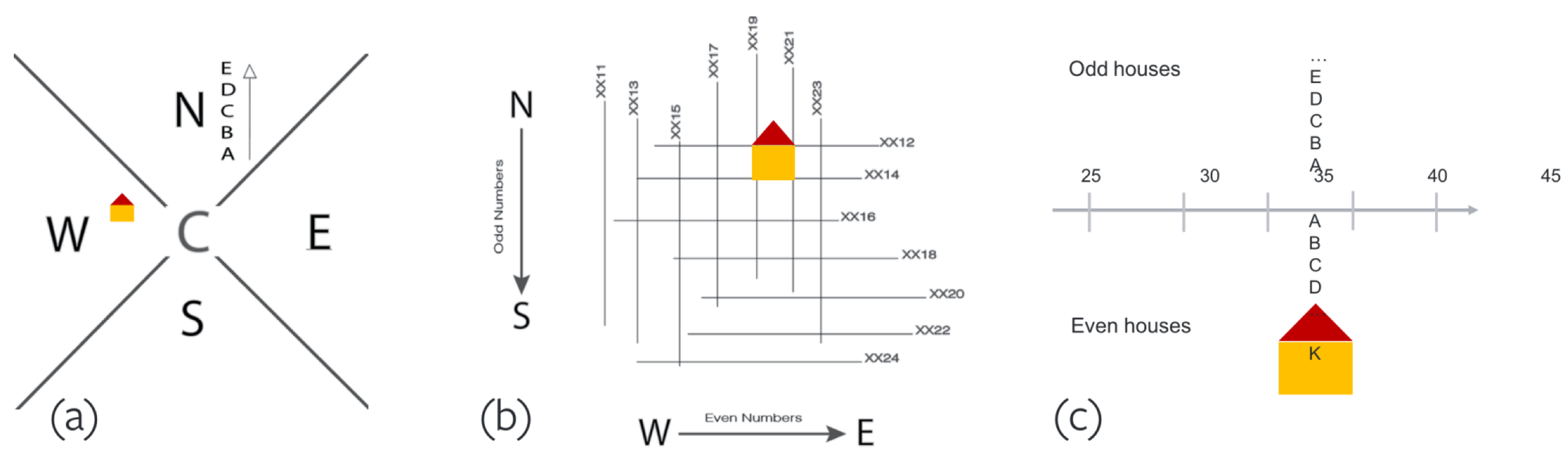
- A physical addressing scheme, which is linear, hierarchical, flexible, intuitive, perceptible, and robust.
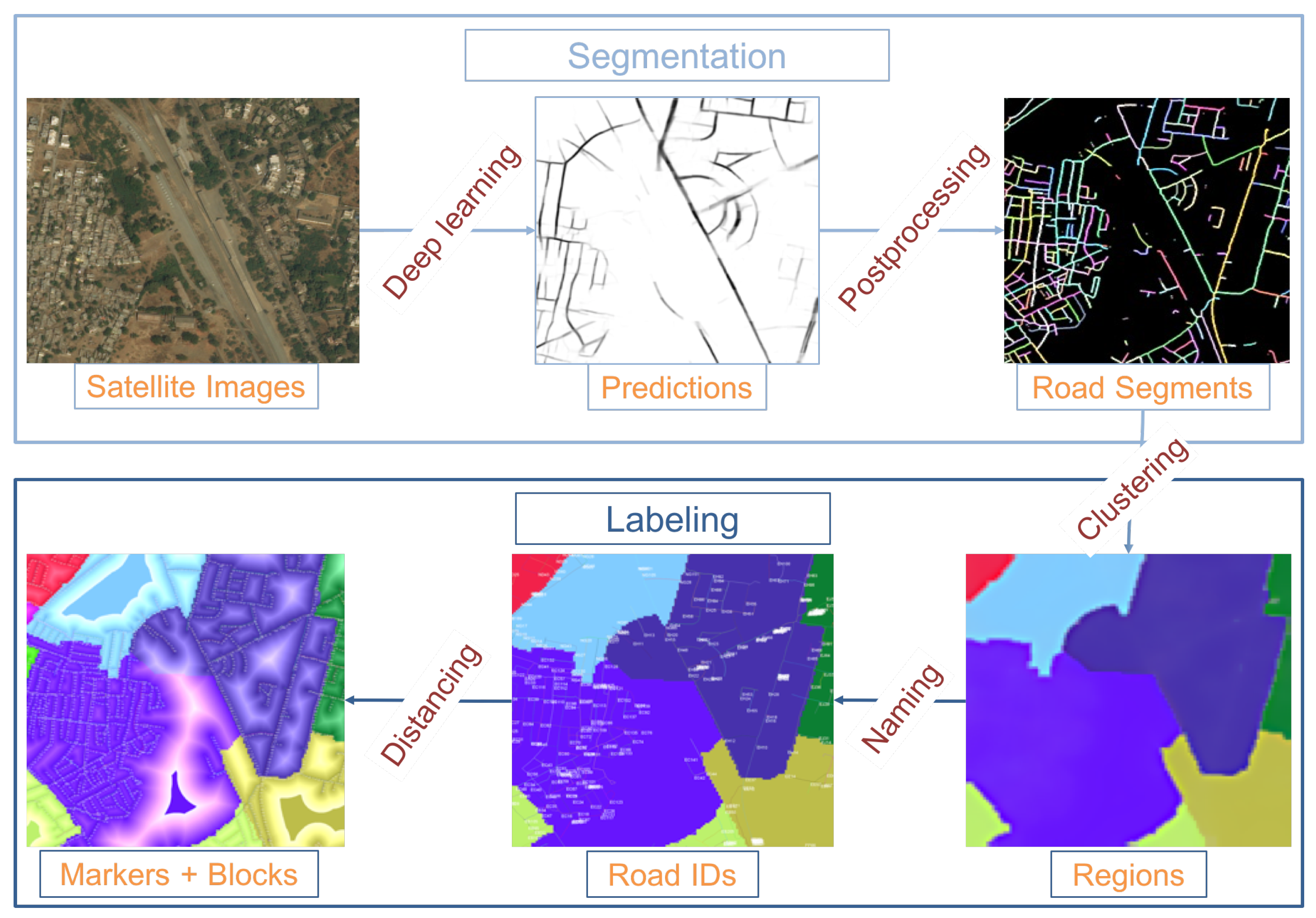
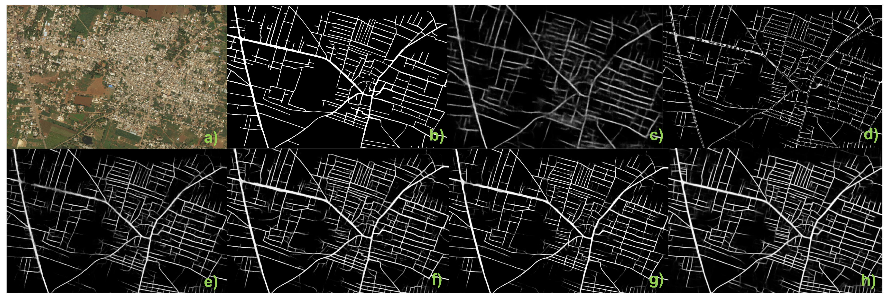
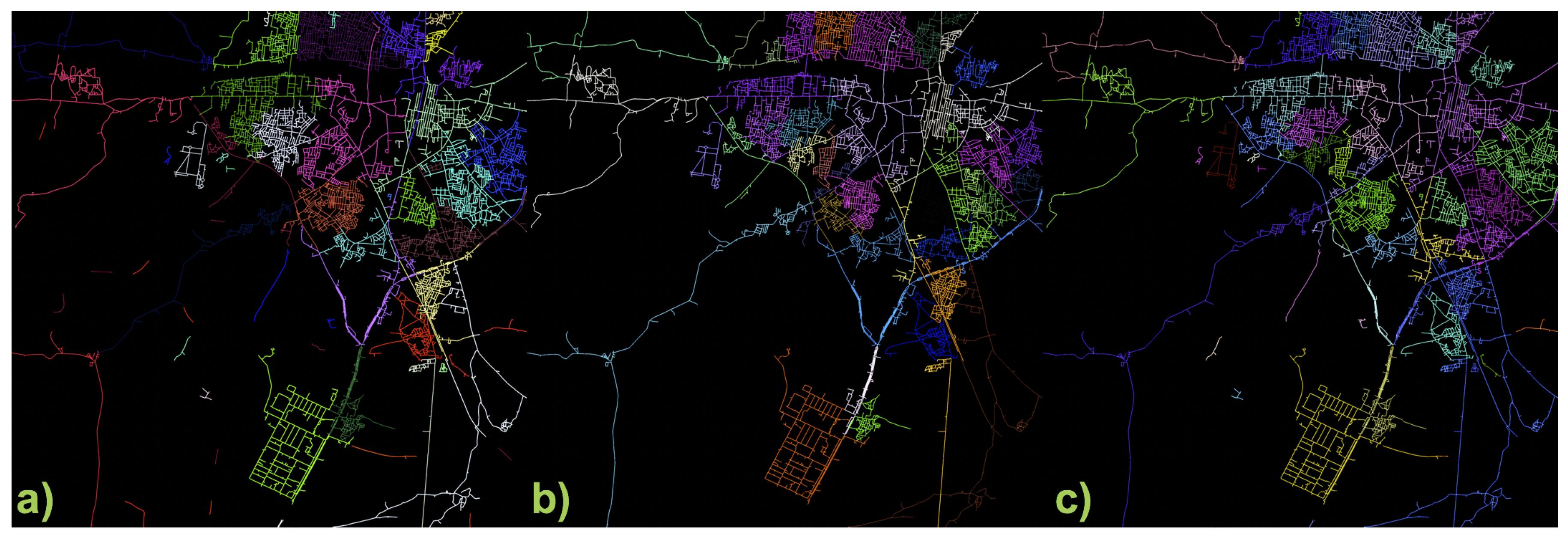
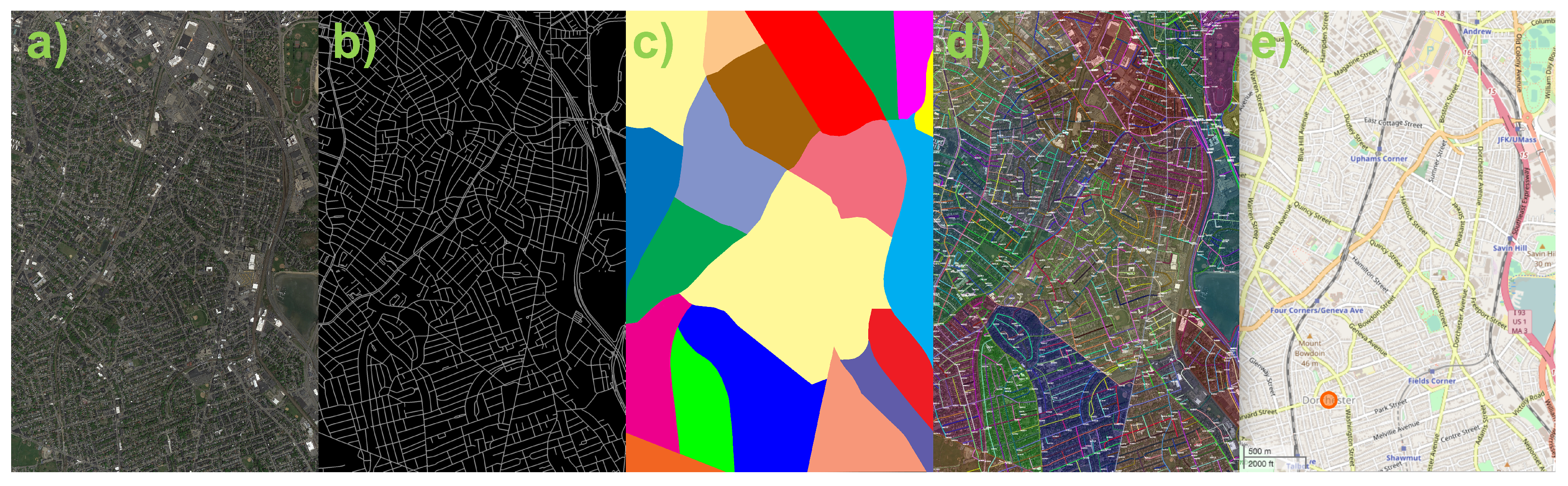
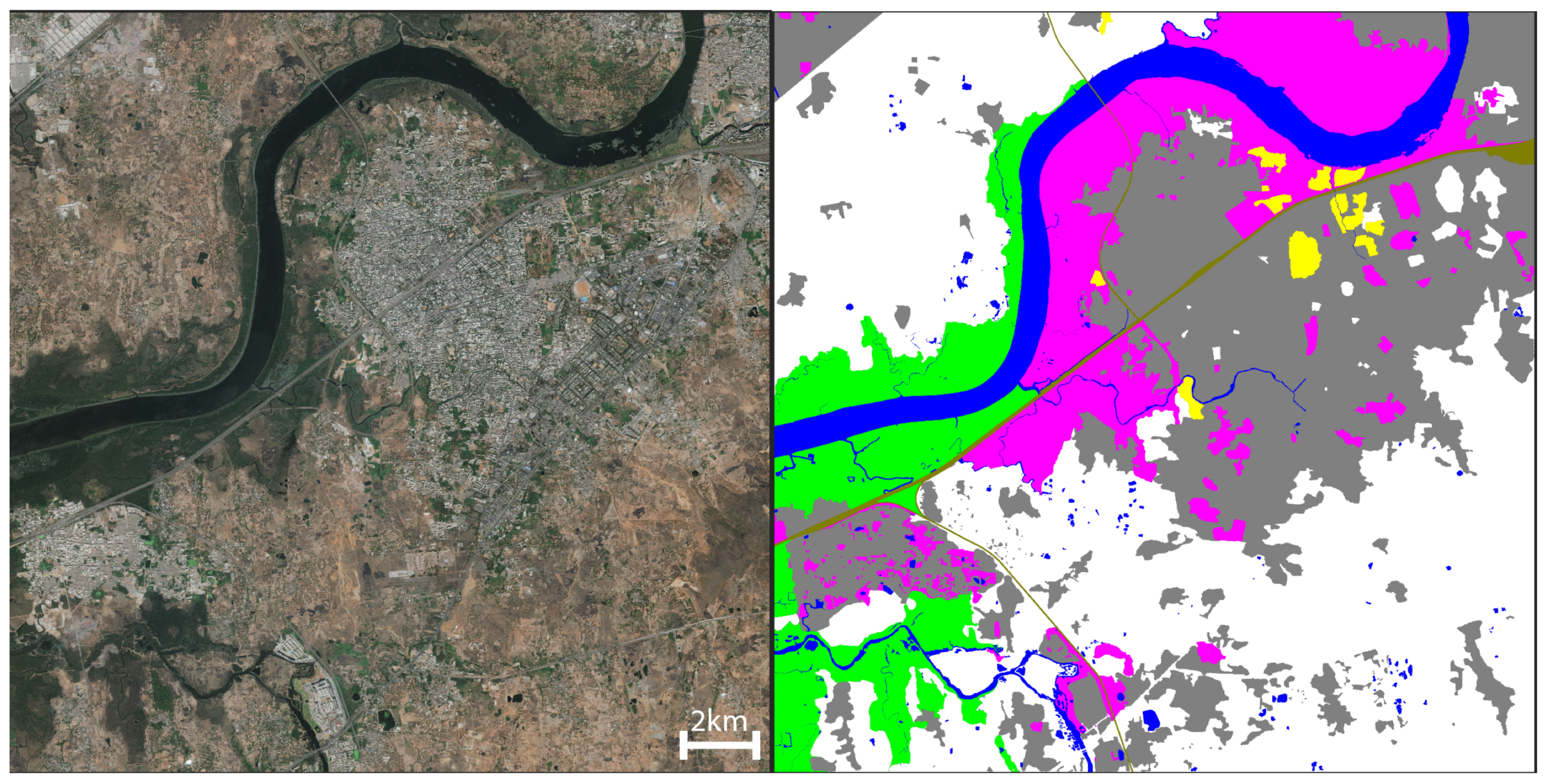
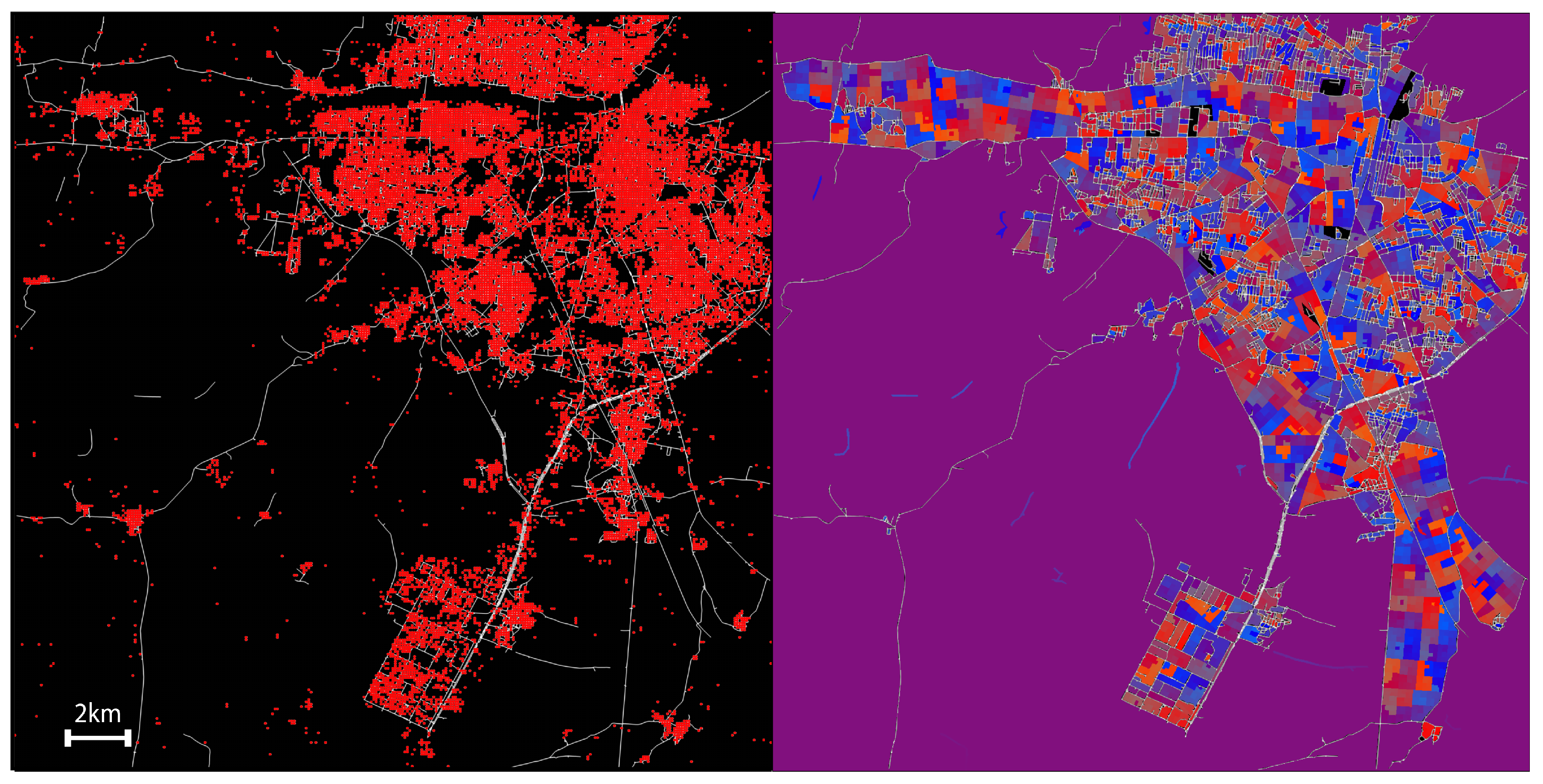
- A segmentation method to obtain road segments and regions from satellite imagery, using deep learning and graph-partitioning algorithms.
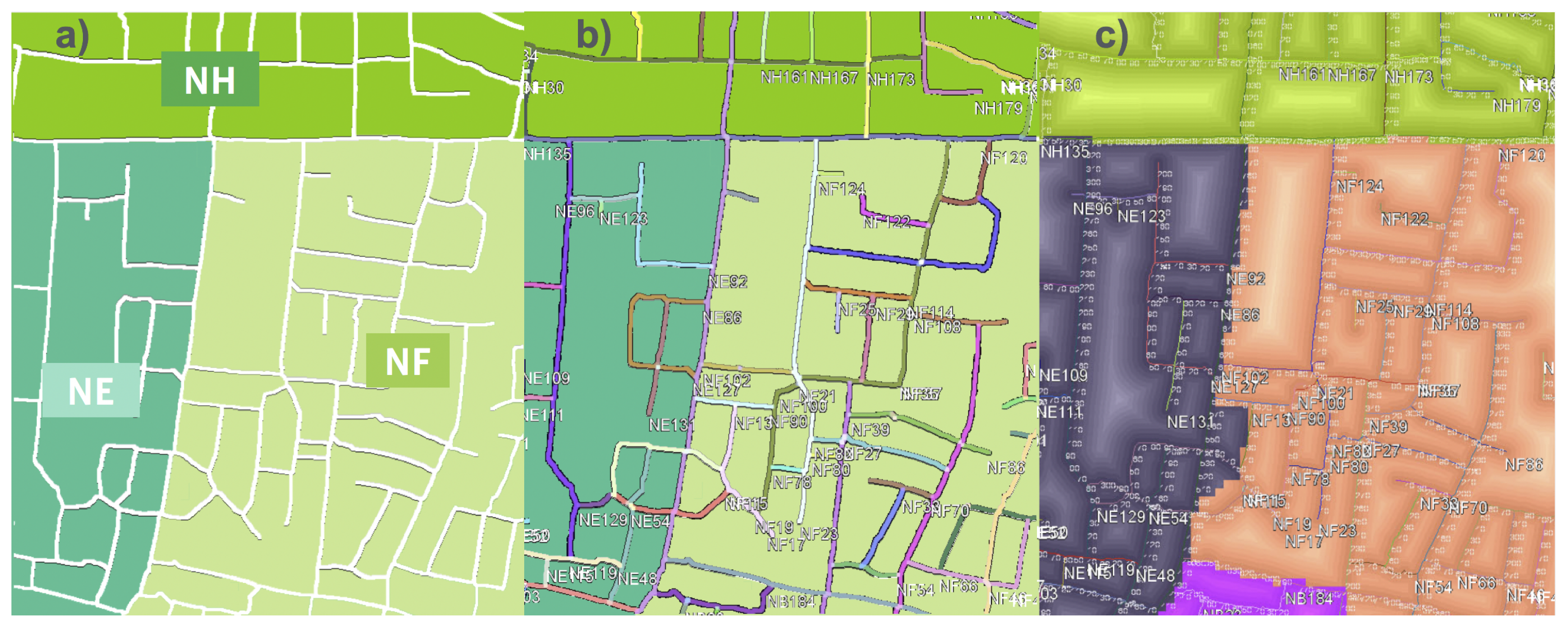
- A labeling method to name urban elements on the basis of current addressing schemes and distance fields.
- A ready-to-deploy prototype application of the generative system supporting forward and inverse geoqueries.
2. Related Work
3. Generative Maps
3.1. Addressing Around the World
3.2. Design Properties
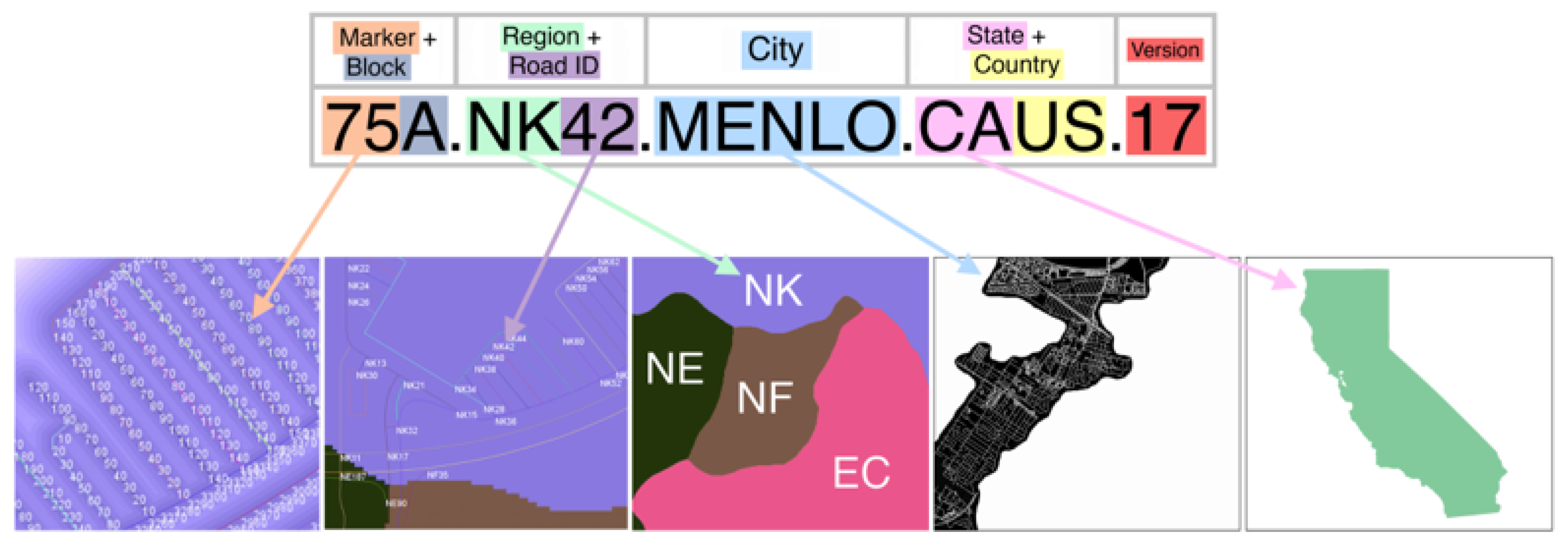
3.3. The Address Format
4. Our Generative Addressing System
4.1. Input and OSM
4.2. Predictive Segmentation
4.3. Region Creation
4.4. Region, Road, and Block Labeling
4.5. Output Formats
5. Inaccessible Areas
5.1. Linear Hashing
5.2. Hierarchical Hashing
6. Results and Applications
7. Extensions and Discussion
7.1. Determinism, Repeatability, and Complexity Analysis
7.2. A Global Address Space: Place Name Server
7.3. Other Extensions
7.3.1. Versioning and Updates
7.3.2. Missing City Boundaries
7.3.3. Overflowing Regions
7.3.4. Roads in 3D
8. Limitations and Future Work
9. Conclusions
Acknowledgments
Author Contributions
Conflicts of Interest
References
- Jones, G.R. Human Friendly Coordinates. GeoInformatics 2015, 18, 10–12. [Google Scholar]
- OpenStreetMap. Haiti Project. 2011. Available online: https://hotosm.org/projects/haiti-2 (accessed on 11 December 2017).
- Open Location Code: An Open Source Standard for Addresses, Independent of Building Numbers and Street Names. Available online: https://github.com/google/open-location-code/blob/master/docs/olc_definition.adoc (accessed on 1 December 2017).
- Zhang, A.; Gros, A.; Tiecke, T.; Liu, X. Population Density Estimation with Deconvolutional Neural Networks. In Proceedings of the Workshop on Large Scale Computer Vision at NIPS, Barcelona, Spain, 5–10 December 2016. [Google Scholar]
- Demir, I.; Hughes, F.; Raj, A.; Tsourides, K.; Ravichandran, D.; Murthy, S.; Dhruv, K.; Garg, S.; Malhotra, J.; Doo, B.; Kermani, G.; Raskar, R. Robocodes: Towards Generative Street Addresses from Satellite Imagery. In Proceedings of the IEEE International Conference on Computer Vision and Pattern Recognition Workshops, Honolulu, HI, USA, 21–26 July 2017. [Google Scholar]
- What Is the Right Addressing Scheme for India? Available online: http://mitemergingworlds.com/blog/2017/11/22/what-is-the-right-addressing-scheme-for-india (accessed on 1 December 2017).
- Chen, G.; Esch, G.; Wonka, P.; Müller, P.; Zhang, E. Interactive Procedural Street Modeling. ACM Trans. Graph. 2008, 27, 103. [Google Scholar] [CrossRef]
- Vanegas, C.A.; Kelly, T.; Weber, B.; Halatsch, J.; Aliaga, D.G.; Muller, P. Procedural Generation of Parcels in Urban Modeling. Comput. Graph. Forum 2012, 31, 681–690. [Google Scholar] [CrossRef]
- Parish, Y.I.H.; Müller, P. Procedural Modeling of Cities. In Proceedings of the 28th Annual Conference on Computer Graphics and Interactive Techniques (SIGGRAPH ’01), Los Angeles, CA, USA, 12–17 August 2001; ACM: New York, NY, USA, 2001; pp. 301–308. [Google Scholar]
- Aliaga, D.G.; Vanegas, C.A.; Benes, B. Interactive Example-based Urban Layout Synthesis. ACM Trans. Graph. 2008, 27, 160. [Google Scholar] [CrossRef]
- Sun, J.; Yu, X.; Baciu, G.; Green, M. Template-based Generation of Road Networks for Virtual City Modeling. In Proceedings of the ACM Symposium on Virtual Reality Software and Technology (VRST ’02), Hong Kong, China, 11–13 November 2002; ACM: New York, NY, USA, 2002; pp. 33–40. [Google Scholar]
- Aliaga, D.G.; Demir, I.; Benes, B.; Wand, M. Inverse Procedural Modeling of 3D Models for Virtual Worlds. In Proceedings of the ACM SIGGRAPH 2016 Courses (SIGGRAPH ’16), Anaheim, CA, USA, 24–28 July 2016; ACM: New York, NY, USA, 2016; p. 16. [Google Scholar]
- Wang, Y.; Liu, X.; Wei, H.; Forman, G.; Zhu, Y. CrowdAtlas: Self-updating Maps for Cloud and Personal Use. In Proceedings of the 11th Annual International Conference on Mobile Systems, Applications, and Services (MobiSys ’13), Taipei, Taiwan, 25–28 June 2013; ACM: New York, NY, USA, 2013; pp. 469–470. [Google Scholar]
- Skoumas, G.; Pfoser, D.; Kyrillidis, A.; Sellis, T. Location Estimation Using Crowdsourced Spatial Relations. ACM Trans. Spat. Algorithms Syst. 2016, 2, 5. [Google Scholar] [CrossRef]
- Mattyus, G.; Wang, S.; Fidler, S.; Urtasun, R. Enhancing Road Maps by Parsing Aerial Images around the World. In Proceedings of the 2015 IEEE International Conference on Computer Vision (ICCV), Santiago, Chile, 7–13 December 2015; pp. 1689–1697. [Google Scholar]
- Mattyus, G.; Luo, W.; Urtasun, R. DeepRoadMapper: Extracting Road Topology from Aerial Images. In Proceedings of the IEEE International Conference on Computer Vision (ICCV), Venice, Italy, 22–29 October 2017. [Google Scholar]
- Zeng, D.; Zhang, T.; Fang, R.; Shen, W.; Tian, Q. Neighborhood geometry based feature matching for geostationary satellite remote sensing image. Neurocomputing 2017, 236, 65–72. [Google Scholar] [CrossRef]
- Wang, J.; Song, J.; Chen, M.; Yang, Z. Road network extraction: A neural-dynamic framework based on deep learning and a finite state machine. Int. J. Remote Sens. 2015, 36, 3144–3169. [Google Scholar] [CrossRef]
- Zhao, J.; You, S. Road network extraction from airborne LiDAR data using scene context. In Proceedings of the 2012 IEEE Computer Society Conference on Computer Vision and Pattern Recognition Workshops, Providence, RI, USA, 16–21 June 2012; pp. 9–16. [Google Scholar]
- Li, P.; Zang, Y.; Wang, C.; Li, J.; Cheng, M.; Luo, L.; Yu, Y. Road network extraction via deep learning and line integral convolution. In Proceedings of the 2016 IEEE International Geoscience and Remote Sensing Symposium (IGARSS), Beijing, China, 10–15 July 2016; pp. 1599–1602. [Google Scholar]
- Xu, L.; Jun, T.; Xiang, Y.; JianJie, C.; LiQian, G. The rapid method for road extraction from high-resolution satellite images based on USM algorithm. In Proceedings of the 2012 International Conference on Image Analysis and Signal Processing, Hangzhou, China, 9–11 November 2012; pp. 1–6. [Google Scholar]
- Peteri, R.; Celle, J.; Ranchin, T. Detection and extraction of road networks from high resolution satellite images. In Proceedings of the 2003 International Conference on Image Processing, Barcelona, Spain, 14–17 September 2003; Volume 1. [Google Scholar] [CrossRef]
- Poullis, C.; You, S.; Neumann, U. A Vision-Based System For Automatic Detection and Extraction of Road Networks. In Proceedings of the 2008 IEEE Workshop on Applications of Computer Vision, Copper Mountain, CO, USA, 7–9 January 2008; pp. 1–8. [Google Scholar]
- Wegner, J.D.; Montoya-Zegarra, J.A.; Schindler, K. A Higher-Order CRF Model for Road Network Extraction. In Proceedings of the 2013 IEEE Conference on Computer Vision and Pattern Recognition, Portland, OR, USA, 23–28 June 2013; pp. 1698–1705. [Google Scholar]
- Alshehhi, R.; Marpu, P.R. Hierarchical graph-based segmentation for extracting road networks from high-resolution satellite images. ISPRS J. Photogramm. Remote Sens. 2017, 126, 245–260. [Google Scholar] [CrossRef]
- Anwar, T.; Liu, C.; Vu, H.L.; Leckie, C. Partitioning road networks using density peak graphs: Efficiency vs. accuracy. Inf. Syst. 2017, 64, 22–40. [Google Scholar] [CrossRef]
- An Entire Village Gets Street Names. 2016. Available online: http://mitemergingworlds.com/blog/2016/8/14/an-entire-village-gets-street-names (accessed on 1 December 2017).
- Economic Impact of Discoverability. 2018. Available online: http://mitemergingworlds.com/blog/2018/2/12/economic-impact-of-discoverability-of-localities-and-addresses-in-india (accessed on 15 February 2018).
- Tian, Q.; Ren, F.; Hu, T.; Liu, J.; Li, R.; Du, Q. Using an Optimized Chinese Address Matching Method to Develop a Geocoding Service: A Case Study of Shenzhen, China. ISPRS Int. J. Geo-Inf. 2016, 5, 65. [Google Scholar] [CrossRef]
- Weihong, L.; Ao, Z.; Kan, D. An Efficient Bayesian Framework Based Place Name Segmentation Algorithm for Geocoding System. In Proceedings of the 2014 Fifth International Conference on Intelligent Systems Design and Engineering Applications, Zhangjiajie, Hunan, China, 15–16 June 2014; pp. 141–144. [Google Scholar]
- The City of London. London Postal Code System. 2016. Available online: https://www.london.gov.uk/sites/default/files/gla_postcode_map_a3_map1.pdf (accessed on 1 December 2017).
- London Postal Codes. Available online: https://www.doogal.co.uk/londonpostcodes.php (accessed on 1 December 2017).
- Ministry of the Interior and Safety—Map Services. Available online: http://www.juso.go.kr/support/AddressMainSearch2.do (accessed on 1 December 2017).
- Berliner Hausnummern. Available online: https://hausnummern.tagesspiegel.de (accessed on 1 December 2017).
- Farvacque-Vitkovic, C.; Godin, L.; Leroux, H.; Verdet, F.; Chavez, R. (Eds.) Street Addressing and the Management of Cities; World Bank: Washington, DC, USA, 2005; p. xvi. 264p. [Google Scholar]
- DigitalGlobe. Available online: https://www.digitalglobe.com/ (accessed on 1 December 2017).
- OpenStreetMap. Available online: openstreetmap.org (accessed on 1 December 2017).
- Badrinarayanan, V.; Kendall, A.; Cipolla, R. SegNet: A Deep Convolutional Encoder-Decoder Architecture for Image Segmentation. arXiv, 2015; arXiv:1511.00561. [Google Scholar]
- Simonyan, K.; Zisserman, A. Very Deep Convolutional Networks for Large-Scale Image Recognition. arXiv, 2014; arXiv:1409.1556. [Google Scholar]
- Ronneberger, O.; Fischer, P.; Brox, T. U-Net: Convolutional Networks for Biomedical Image Segmentation. arXiv, 2015; arXiv:1505.04597. [Google Scholar]
- He, K.; Zhang, X.; Ren, S.; Sun, J. Deep Residual Learning for Image Recognition. In Proceedings of the 2016 IEEE Conference on Computer Vision and Pattern Recognition (CVPR), Las Vegas, NV, USA, 27–30 June 2016; pp. 770–778. [Google Scholar]
- Chen, L.C.; Papandreou, G.; Kokkinos, I.; Murphy, K.; Yuille, A.L. DeepLab: Semantic Image Segmentation with Deep Convolutional Nets, Atrous Convolution, and Fully Connected CRFs. IEEE Trans. Pattern Anal. Mach. Intell. 2017, PP, 1. [Google Scholar] [CrossRef] [PubMed]
- Sironi, A.; Lepetit, V.; Fua, P. Multiscale Centerline Detection by Learning a Scale-Space Distance Transform. In Proceedings of the 2014 IEEE Conference on Computer Vision and Pattern Recognition, Columbus, OH, USA, 23–28 June 2014; pp. 2697–2704. [Google Scholar]
- Yu, S.X.; Shi, J. Multiclass Spectral Clustering. In Proceedings of the Ninth IEEE International Conference on Computer Vision (ICCV ’03), Nice, France, 13–16 October 2003; IEEE Computer Society: Washington, DC, USA, 2003; Volume 2, p. 313. [Google Scholar]
- Girvan, M.; Newman, M.E. Community structure in social and biological networks. Proc. Natl. Acad. Sci. USA 2002, 99, 7821–7826. [Google Scholar] [CrossRef] [PubMed]
- Blondel, V.D.; Guillaume, J.L.; Lambiotte, R.; Lefebvre, E. Fast unfolding of communities in large networks. J. Stat. Mech. Theory Exp. 2008, 2008, P10008. [Google Scholar] [CrossRef]
- Modha, D.S.; Spangler, W.S. Feature Weighting in K-Means Clustering. Mach. Learn. 2003, 52, 217–237. [Google Scholar] [CrossRef]
- Li, Z.; Chen, J. Superpixel segmentation using Linear Spectral Clustering. In Proceedings of the 2015 IEEE Conference on Computer Vision and Pattern Recognition (CVPR), Boston, MA, USA, 7–12 June 2015; pp. 1356–1363. [Google Scholar]
- Comaniciu, D.; Meer, P. Mean shift: A robust approach toward feature space analysis. IEEE Trans. Pattern Anal. Mach. Intell. 2002, 24, 603–619. [Google Scholar] [CrossRef]
- Tokui, S.; Oono, K.; Hido, S.; Clayton, J. Chainer: A Next-Generation Open Source Framework for Deep Learning. In Proceedings of the Workshop on Machine Learning Systems (LearningSys) in the Twenty-Ninth Annual Conference on Neural Information Processing Systems (NIPS), Montreal, QC, Canada, 7–12 December 2015. [Google Scholar]


| City | Population (per Tile) | Density (mile per City) ) |
|---|---|---|
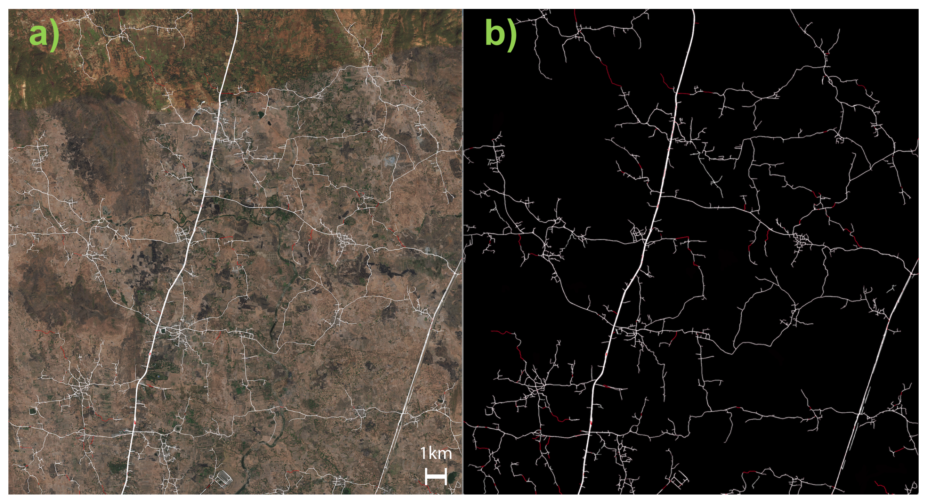
| Figure 1 | 65,000 | 2755 |
| Figure 11 | 100,000 | 13,660 |
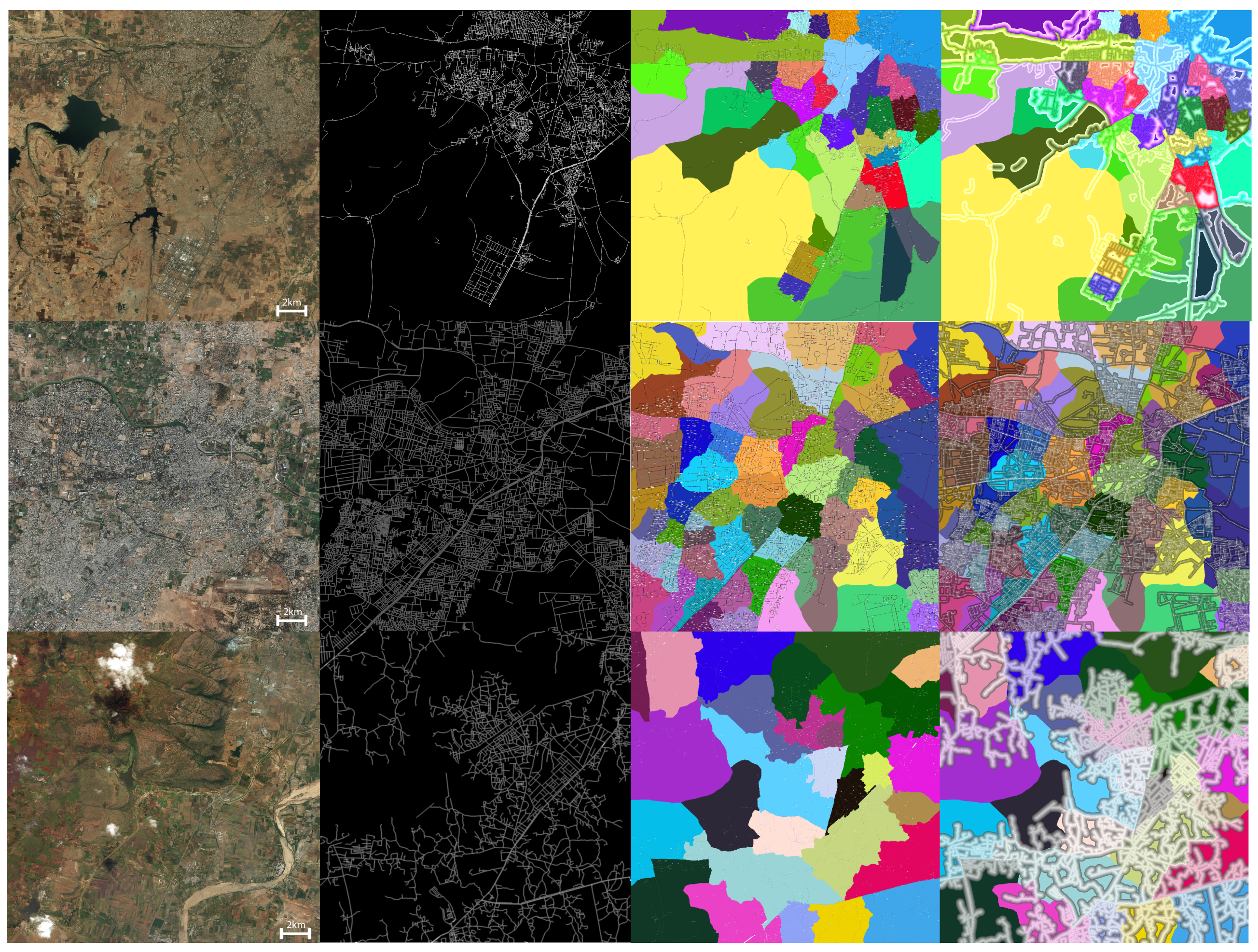
| Figure 12 (top) | 31,000 | 740 |
| Figure 12 (middle) | 116,000 | 6200 |
| Figure 12 (bottom) | 26,000 | 8430 |
© 2018 by the authors. Licensee MDPI, Basel, Switzerland. This article is an open access article distributed under the terms and conditions of the Creative Commons Attribution (CC BY) license (http://creativecommons.org/licenses/by/4.0/).
Share and Cite
Demir, İ.; Hughes, F.; Raj, A.; Dhruv, K.; Muddala, S.M.; Garg, S.; Doo, B.; Raskar, R. Generative Street Addresses from Satellite Imagery. ISPRS Int. J. Geo-Inf. 2018, 7, 84. https://doi.org/10.3390/ijgi7030084
Demir İ, Hughes F, Raj A, Dhruv K, Muddala SM, Garg S, Doo B, Raskar R. Generative Street Addresses from Satellite Imagery. ISPRS International Journal of Geo-Information. 2018; 7(3):84. https://doi.org/10.3390/ijgi7030084
Chicago/Turabian StyleDemir, İlke, Forest Hughes, Aman Raj, Kaunil Dhruv, Suryanarayana Murthy Muddala, Sanyam Garg, Barrett Doo, and Ramesh Raskar. 2018. "Generative Street Addresses from Satellite Imagery" ISPRS International Journal of Geo-Information 7, no. 3: 84. https://doi.org/10.3390/ijgi7030084
APA StyleDemir, İ., Hughes, F., Raj, A., Dhruv, K., Muddala, S. M., Garg, S., Doo, B., & Raskar, R. (2018). Generative Street Addresses from Satellite Imagery. ISPRS International Journal of Geo-Information, 7(3), 84. https://doi.org/10.3390/ijgi7030084