Article

Generative Street Addresses from Satellite Imagery

1
Facebook, 1 Hacker Way, Meenlo Park, CA 94025, USA
2
MIT Media Lab, 75 Amherst St, Cambridge, MA 02139, USA
*
Author to whom correspondence should be addressed.
ISPRS Int. J. Geo-Inf. 2018, 7(3), 84; https://doi.org/10.3390/ijgi7030084
Submission received: 9 January 2018 / Revised: 13 February 2018 / Accepted: 17 February 2018 / Published: 8 March 2018
(This article belongs to the Special Issue Machine Learning for Geospatial Data Analysis)

Abstract

:
We describe our automatic generative algorithm to create street addresses from satellite images by learning and labeling roads, regions, and address cells. Currently, 75% of the world’s roads lack adequate street addressing systems. Recent geocoding initiatives tend to convert pure latitude and longitude information into a memorable form for unknown areas. However, settlements are identified by streets, and such addressing schemes are not coherent with the road topology. Instead, we propose a generative address design that maps the globe in accordance with streets. Our algorithm starts with extracting roads from satellite imagery by utilizing deep learning. Then, it uniquely labels the regions, roads, and structures using some graph- and proximity-based algorithms. We also extend our addressing scheme to (i) cover inaccessible areas following similar design principles; (ii) be inclusive and flexible for changes on the ground; and (iii) lead as a pioneer for a unified street-based global geodatabase. We present our results on an example of a developed city and multiple undeveloped cities. We also compare productivity on the basis of current ad hoc and new complete addresses. We conclude by contrasting our generative addresses to current industrial and open solutions.

1. Introduction

Currently 75% of the roads in the world are not mapped [1], and this number is increasing in developing countries. This problem is more critical in disaster zones, as even aid agencies struggle to agree on names for streets. For example, after the Haiti earthquake, the OpenStreetMap (OSM) community started processing satellite imagery to track the roads within 48 h [2]. After 6 months, the same map became the default resource for rescue teams, non-governmental organizations, and the United Nations. On the other hand, while the technology to conduct remote sensing has been significantly improving over the past decade, the organic growth of urban and suburban areas outruns the deployment of addressing schemes. Street addresses enhance precise physical presence and effectively increase the connectivity all around the world. We imagine an algorithm that creates such meaningful addresses for unmapped places in the world that have no street name or address. We are introducing an automatic algorithm to accomplish this task, using machine learning and computer vision approaches fed with satellite imagery.
Generative labeling is key for many areas, such as natural language processing, semantic labeling, and inverse procedural modeling. Applying a generative scheme to unlabeled streets can dramatically simplify map generation for digital tasks while at the same time providing a testbed to grow meaningful and intuitive street assignments. The automation of address creation enables spatial information to be encoded and represented much more efficiently, providing a topologically coherent graph around the world that can be used by many geoapplications.
Recent initiatives (e.g., what3words [1], plus codes [3], etc.) try to accomplish this task by automatic geocoding. Although these solutions can encode and compress spatial data, geocodes do not contain the inherent properties held by street addresses. For example, they are not intuitive for directional and proximity queries, they tend to be decoupled from the true road topology, and they often may not be coherent with human perception. A unified representation of all street addresses around the world can serve as an alternative for the regular grid of geocodes to a more natural grid of roads and can help to organize the world in more natural ways.
In order to realize this, we have constructed a generative addressing system (see Figure 1) to bridge the gap between grid-based digital addressing schemes and traditional street addresses. Merging the two extents, we have designed an addressing scheme that follows a set of properties. In order to automatically generate such street addresses, we have developed a system to learn regions, roads, and blocks from satellite images to utilize artificial intelligence in mapping. Our main contributions include the following:
  • A physical addressing scheme, which is linear, hierarchical, flexible, intuitive, perceptible, and robust.
  • A segmentation method to obtain road segments and regions from satellite imagery, using deep learning and graph-partitioning algorithms.
  • A labeling method to name urban elements on the basis of current addressing schemes and distance fields.
  • A ready-to-deploy prototype application of the generative system supporting forward and inverse geoqueries.
We have compared our generated maps to existing commercial and open maps by analyzing our addressing scheme on (i) already fully mapped areas for validation hierarchical labeling; and (ii) unmapped areas for the evaluation of road segments and region extraction. We have also evaluated the intuitiveness and utility of our new addressing system on multiple areas of unmapped territories, comparing travel times using old and new addresses. We have verified our map extraction algorithm using the population density [4] of some example areas. On the basis of the comparisons, analysis, and the user feedback, we observed that our system was able to provide accurate maps for 85% percent of the test cases, improving by 20% over the currently existing maps, and decrease the travel times by 60% on average.

2. Related Work

In this section, we look into available addressing schemes and generative approaches followed by related works of some stages of our pipeline. This paper builds upon our previous approach [5] to create a complete system with extensions, improved models, new results, and solutions for edge cases.
The geocoding process involves converting latitude and longitude information, approximated up to a percentile, into a unique code. A quick investigation among popular geocoding solutions can reveal that such codes are either not in human-readable form (e.g., GooglePlaceID and OkHi) or they tend to de-correlate from the true topological information (e.g., [1], Zippr and MapTags). While these solutions can encode and compress spatial data efficiently, such geocodes do not contain the essential properties of a street addressing system, such as linearity and hierarchy. Similar geocoding solutions also lack intuitive directionality and proximity information, they are decoupled from the true road topology, and they are incoherent with human perception. Such inherent properties become even more crucial in developing countries, as was shown in a comprehensive analysis [6]. While we also seek an automated approach, at the same time, we want the addresses to follow what is physcially present on the earth.
On the other hand, automating the generation of maps is extensively studied in the urban procedural modeling world. The procedural generation of streets [7], parcels [8], and cities [9] creates detailed and structurally realistic models. However, procedural modeling lacks control, and grammars are mostly written on the basis of domain expertise or flow data and not on the basis of the real world. Taking a step further, other approaches have tried to control the procedural generation by creating and reconfiguring example-based urban layouts [10] or template-based generation [11]. These approaches are powerful generative methods; however, still representing the true road topology is not feasible with such approaches. On the other hand, some inverse procedural modeling (IPM) approaches [12] process real-world data (images, LiDAR, etc.) to extract realistic representations. We follow this last path and rely on satellite imagery for the segmentation and labeling steps of our IPM-like system.
Following the example-based generation idea, another approach to automate the extraction of geospatial information is to use already existing data resources, such as GPS trails [13], user check-ins [14], aerial images [15,16], or geostationary satellite images [17]. Inspired from these approaches, we extract the urban elements of a particular area from satellite images using deep learning to capture their representative features. Similar approaches extract road networks using neural networks for dynamic environments [18] from LiDAR data [19], using line integrals [20] and using image processing approaches [21,22,23]. In our approach, to provide scalability across countries and terrains, we have explored and modified state-of-the-art image segmentation networks. Finally, processing the road topology has been studied as an example case for novel or modified clustering and graph partitioning approaches [24,25,26]. Being a generative approach, our case differs from the previous cases by the ill-posed definition of “regions”. In addition to the original problem being NP-hard, the underconstrained definition of regions adds another layer of complexity. We have suggested our own partitioner in Section 4.2.
Being a human-centric process, labeling such urban structures has also been a challenge [27,28]. Some approaches attempt to name places by address matching [29] or by address segmentation from textual information [30]; however, these methods are based on human input, and thus are not coherent with the physical information. In contrast, after the urban structure is extracted, we label its elements according to our address format, which performs as a bridge between automation and human-friendly addresses.

3. Generative Maps

For our address template, we have defined related design properties for the new address format. We first investigate our properties under three categories: semantic, structural, and natural. Then we explain the format of our new addresses.

3.1. Addressing Around the World

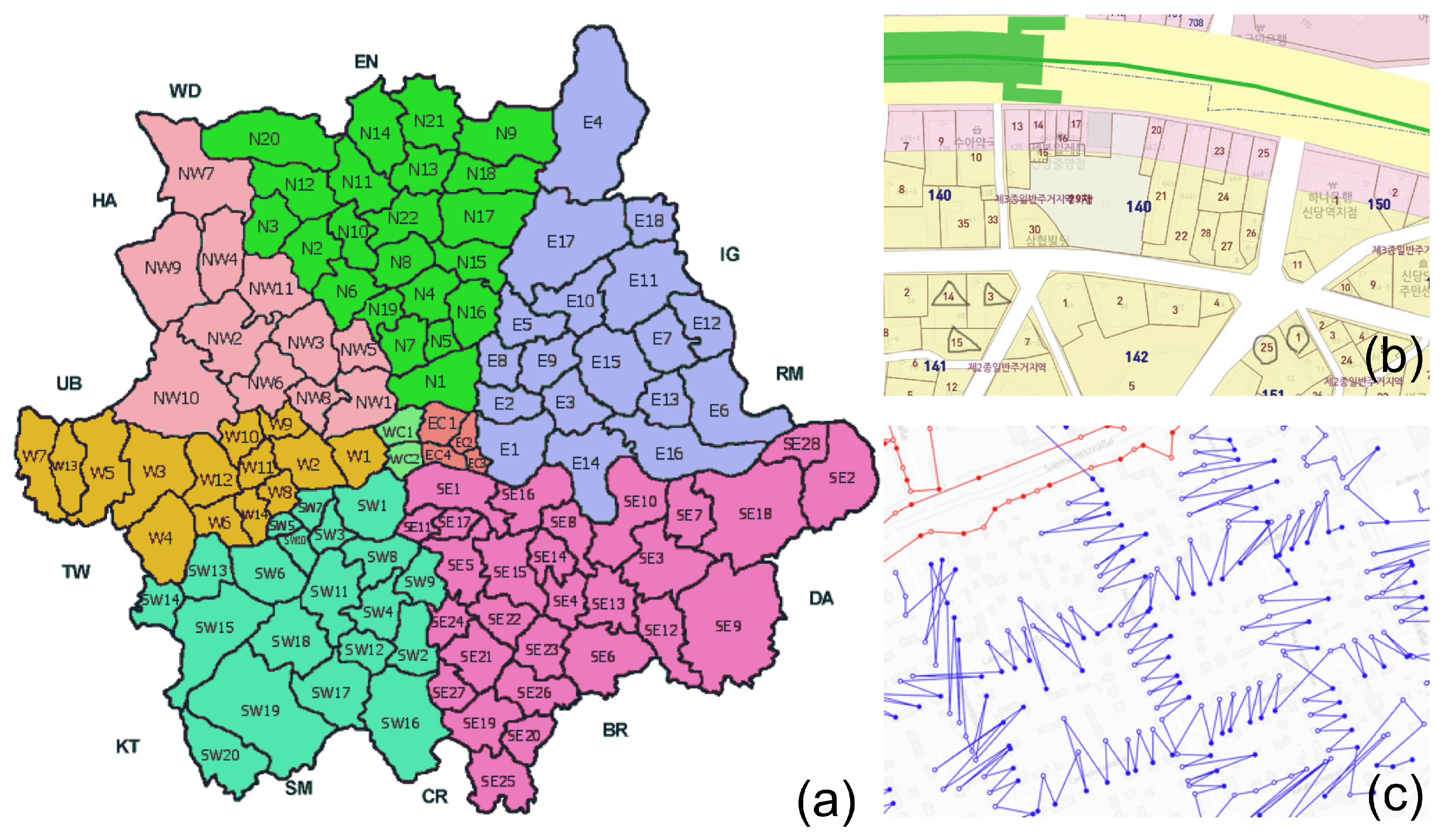
Naturally occurring addresses and names around the world are usually the result of cultural dynamics, politics, economies, and other long-term processes adopted by urban authorities. We want to mimic this organic process, while still maintaining a unified representation that is independent of the human factors. In order to come up with an appropriate scheme, we have conducted some research on the current addressing methods in many countries: for example, the London postal code system [31] (image taken from [32]), which provides orientation- and distance-based radial naming for regions (Figure 2), as well as other schemes, such as South Korea street naming (image taken from [33]), which uses meter markers along the roads, Berlin house numbering (image taken from [34]), which uses zig-zag patterns, and more [35].
We have combined these real-world methodologies to come up with a design to ease the understanding of both humans and machines. Unlike other geocoding efforts, the natural properties within our system allow it to be physically realizable. Labels should be in accordance with natural boundaries, water bodies, and so on. The addresses should also obey the road topology, mimicking real-world addresses. The hierarchical naming within a city boundary is depicted in Figure 3. The yellow house in the example is in a region which is to the west of the downtown with a close distance (“WB” region), on a west-to-east bound street close to the middle of the region (“WB14” street), approximately 190 meters along the street ( 190 / 5 = 38 house number), and approximately 55 meters away from the street (K = 11, 11 5 = 55 apartment number).

3.2. Design Properties

Semantic properties emphasize user-friendly features of our addressing scheme. First, they need to be intuitive for the user regarding their whereabouts. Thus, the addresses should be linear, following the road topology. This linearity concern applies in multiple aspects; that is, consecutive regions, roads, and buildings should have incremental numbers; regions and roads should have a sense of directionality; parallel roads should have the same odd parity; etc. Second, the addresses should be hierarchical in the sense that each hierarchy level reflects scale in terms of location. This hierarchy is both spatial and human-oriented, so that the distance metric is preserved while conserving the boundaries of existing countries and cities. Third, addresses should be universal, memorable, independent of local language and alphabet, short and alphanumeric.
Structural properties enable the format of street addresses to be database and storage friendly. The linear and hierarchical naming should also be preserved in the structural side, in order to keep the querying and updating of records manageable. The addresses should be compressible and easily represented by primitive data types, with a maximum five characters of four words, equaling less than 25 bytes. The addressing scheme should also be robust and extendible, allowing the addressable physical spaces to grow and adapt over time. Thus, the leftover bytes are allocated as a pointer space to future addresses, if needed. Lastly, addresses should enable easy querying in a variety of aspects, such as geometric, proximity-based and type-ahead queries.

3.3. The Address Format

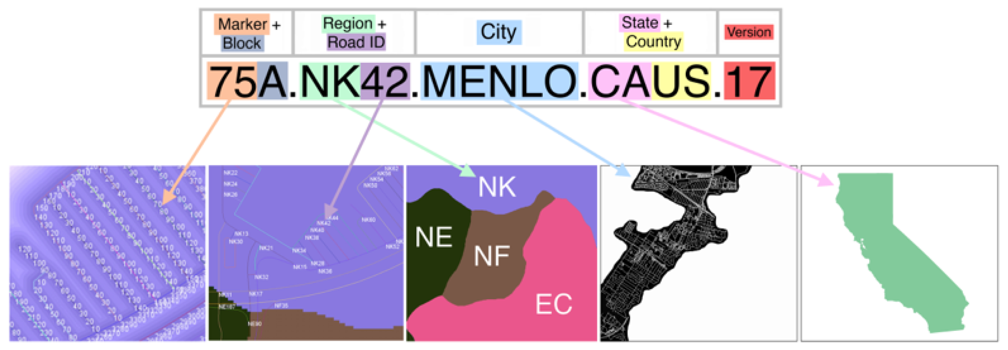
Figure 4 summarizes the aforementioned desired properties. The last field indicates the year that the address is generated. The fourth field contains the country and state information when applicable, preceded by the city information in the third field. Up to this point, the addresses reflect the hierarchical aspect of the maps, on the basis of consensus information around the world. The second field contains the road name, which starts with the region label, followed by the road number. The region label is decided on the basis of the orientation towards the city center in the first character and the distance from the city center in the second character. The roads are numbered according to their directionality and proximity, parallel roads having the same odd parity, and neighboring roads being named consecutively. Lastly, the first field is composed of the meter marker along the road and the block letter from the road, animating the house number and apartment number consecutively, again following the same odd-parity concept for structures on either sides.

4. Our Generative Addressing System

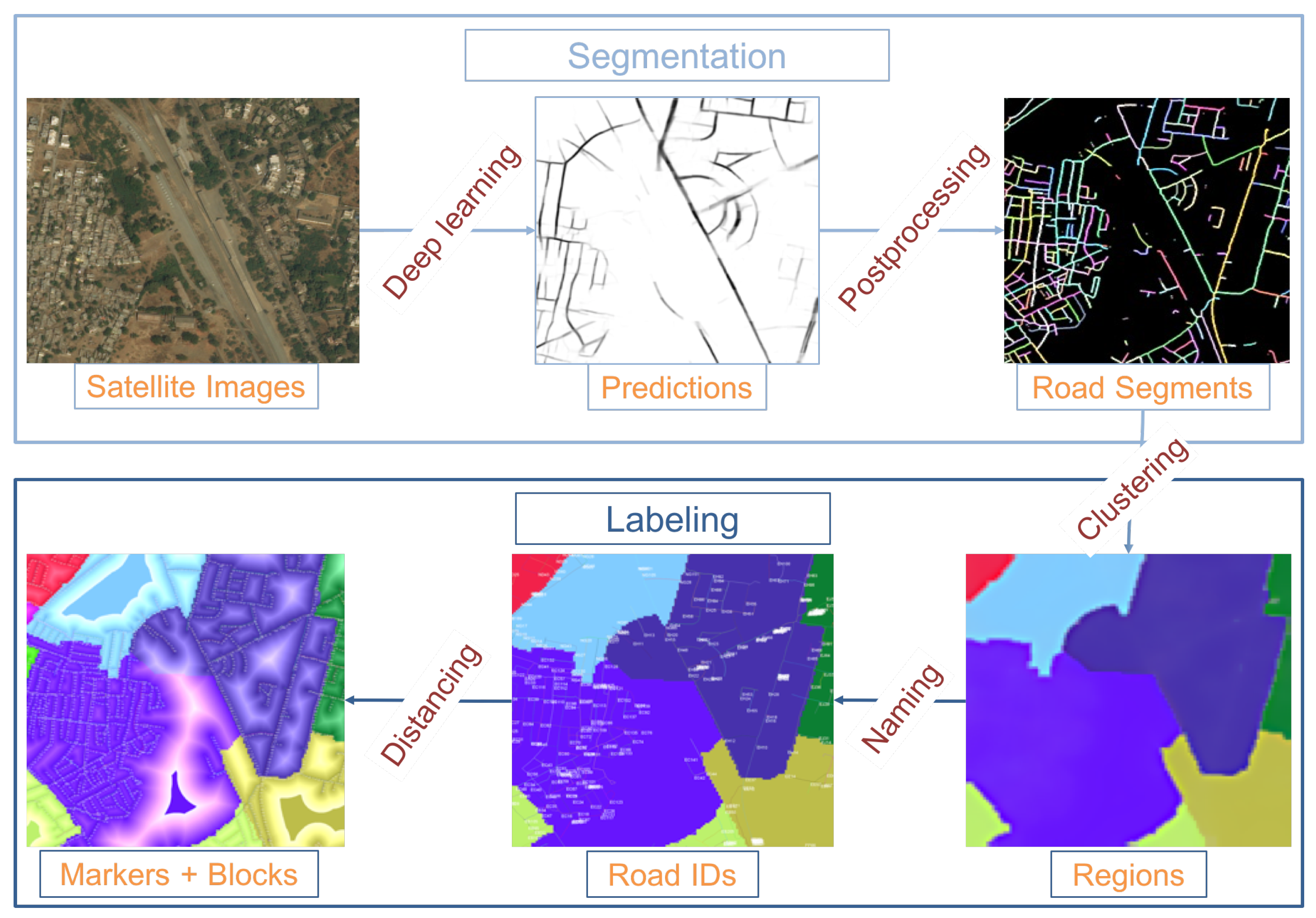
As mentioned in the survey for inverse approaches for urban structures [12], our system follows the general segmentation and labeling steps of inverse procedural modeling. The system pipeline is shown in Figure 5. The segmentation step extracts roads, breaks them into road segments and clusters them into regions. The labeling step names the regions, road segments, and place markers and assigns block letters (26 characters in the English alphabet) to individual addressable units. We explain our algorithmic steps in the following sections.

4.1. Input and OSM

Our model is trained on satellite images of approximately equal to 0.5 m resolution and of size 19 K * 19 K, provided by Digital Globe [36] under a commercial license, but it is also available to the OSM [37] community. The prediction is done per tile; however the rest of the algorithm is executed per city. Thus, we query the city, state, and country boundary information from the OSM and open datasets. In case these datasets do not contain this information, we use our land cover classification model (discussed in Section 7.3.2) to estimate urban areas that can be considered as cities. We also query existing street geometry to augment our road predictions and existing street names to store as pseudo-names for generated street names.

4.2. Predictive Segmentation

The first step of our approach creates binary road prediction images from three channel satellite images. In our system, we modify current state-of-the-art methods in deep learning for our road extraction purpose. Our GIS experts create binary road masks, by manually labeling each pixel as a road or not road. Both training and testing are done with patches of 192 × 192 . The training set includes 4–16 tiles per country, and the test set includes all the rest of the tiles. We split the dataset to train/test in a geographically diverse manner, so that both sets have representative samples. The training and test areas are manually spatially distributed to sample all areas in a country. The number of tiles varies by country, but the ratios of the set sizes are mostly kept at 70% to 30%. We use a modified version of SegNet [38], which consists of the first 13 convolutional layers of the VGG16 network for the encoder, followed by the decoder architecture, having a corresponding decoder layer for each encoder. We modify the last soft-max layer to change the multi-class structure to have binary classes for road detection, by substituting it with a convolutional layer.
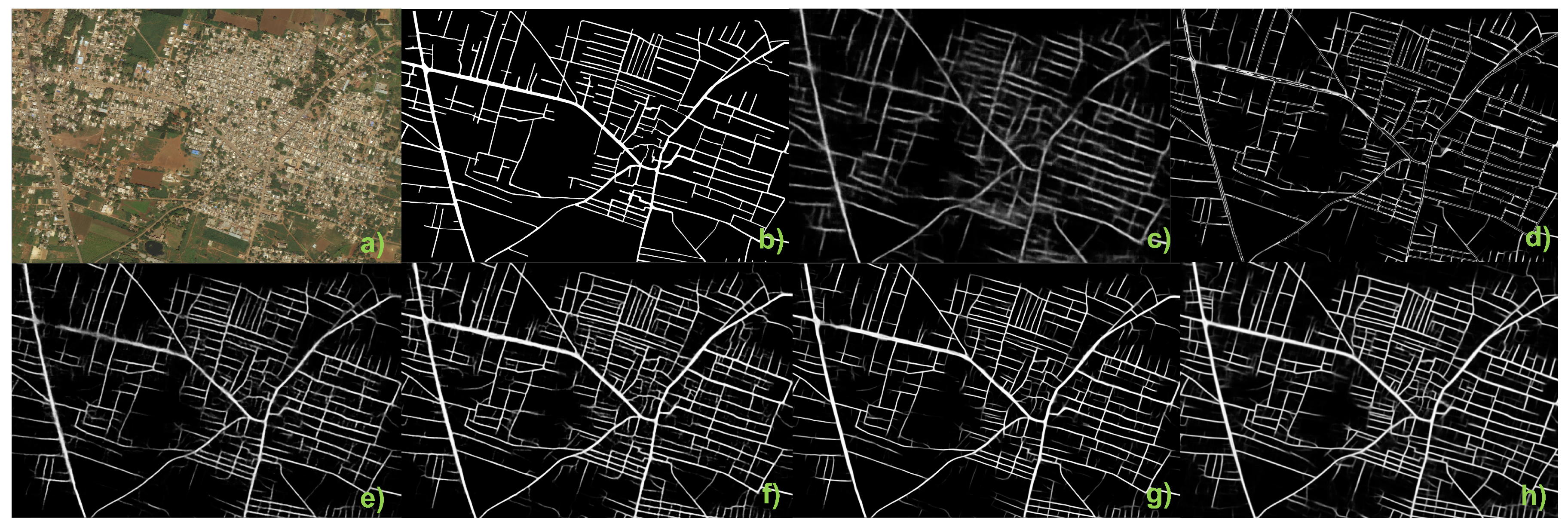
Our approach is flexible enough to accommodate other models. We have also experimented with architectures such as VGG [39] (Figure 6c), U-Net [40] (Figure 6d), and ResNet [41] variations (Figure 6e,f); however, we achieved the best result with the SegNet (Figure 6g) model trained on dense and diverse tiles, resulting in 72.6% precision and 57.2% recall. We experimented with a higher epoch but concluded that 50 was enough, converging in 800 K iterations with a loss of 4.2%. Additionally, in our experiments, SegNet took overall 65% less time during the training phase. The comparison of predictions from different models is shown in Figure 6. The runner-up was the ResNet50 model shown in Figure 6e, with 71.9% precision and 56.3% recall. We have also experimented with DeepLab [42] variations and achieved 75.4% precision and 75.9% recall (Figure 6h); however the model showed signs of overfitting after epoch 30. We leave the discussion about details of this model to another paper.
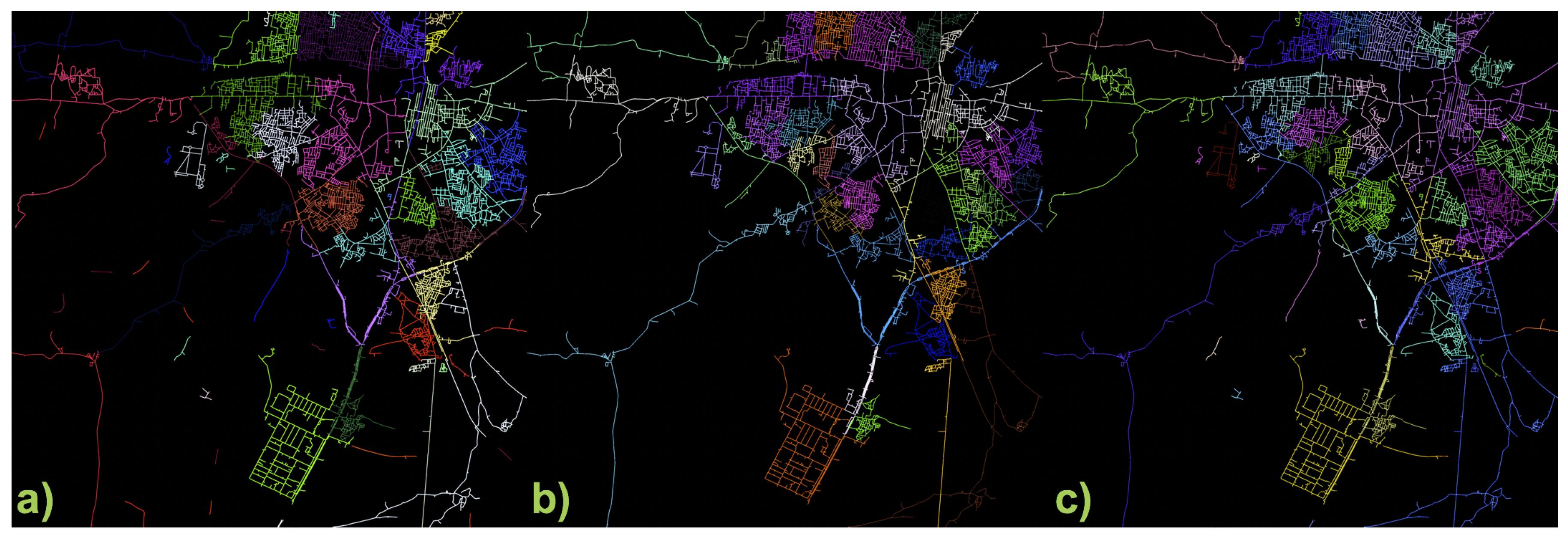
In the next step of our pipeline, we combine the road predictions in a new image with weighted pixels based on confidence. The post-processing step starts by first binarizing the image with thresholding by Otsu’s method. Afterwards, we run a depth-first search with an 8-neighborhood to join connected roads on the basis of the confidences in the original grayscale prediction. Then, we apply an orientation-based adaptive median filtering on the road end points in the processed image, in order to balance preserving the connections and removing the noise. The filter kernel adapts to the direction of the road and amplifies the road along the current direction. If it meets with another road with similar (< ϵ ) direction, then the roads are connected with a curve approximated by the directions at the two end points. Overall, the post-processing approach mimics results such as the centerline extraction method [43]. After merging such broken connections, we divide the roads into road segments on the basis of bucketed orientations. At each intersection, we keep the roads undivided for reciprocal incoming road segments (i.e., horizontal end points of a T-junction); otherwise we add new end points at the intersection to create new road segments (i.e., the intersection of the vertical road with the horizontal at a T-junction). This yields the road segments, consistent with the road topology and land forms. As the last step, we conflate the post-processed road segments with OSM road vectors for better alignment and connectivity, if roads exist in OSM for that area.

4.3. Region Creation

After we have the road segments, we convert them into a road graph in which the nodes correspond to intersections (and end points) and the edges correspond to road segments. We weight the edges on the basis of the segment distance, although some more features (i.e., road width, sift features from the cropped road from the satellite images, etc.) can be easily encoded into the edge weights. We partition the road graph into communities that have the maximum interconnectivity and minimum intraconnectivity. We have experimented with normalized min-cut [44], Newman–Girvan [45], and optimal modularity-based [46] graph partitioning and clustering approaches. Unfortunately, the concept of region is hard to formulate mathematically, and thus we have used the input of our domain experts to evaluate the success of region creation approaches. On the basis of some urban planning rules (i.e., natural boundaries, road distribution, etc.), they have concluded that the regions obtained using min-cut [44] and Newman–Girvan [45] were the closest to real-world regions; thus we chose to use [44], being a significantly more efficient choice. Results of different graph partitioning approaches are demonstrated in Figure 7, where subgraphs of each algorithm is color-coded per example.
For the min-cut parameters, to limit the number of addressable streets within a region, we used n = | r o a d s | / 89 clusters and a third-degree polynomial affinity matrix combined with the weighted adjacency matrix. According to our addressing scheme, we have double-digit street numbers; thus we estimated the number of roads per region as 89 = ( 99 10 ) . Enforcing a probabilistic approach to behave deterministically, we set the number of seeding iterations to a high number (1000) with discretized labels to ensure convergence. We have also experimented with weighted k-means [47], super-pixel [48] and mean-shift [49] segmentations on both the pixelated version of the road graph and on the original and down-sampled satellite images. One intuition behind using graph-partitioning approaches was their being more favorable in clustering the dense regions and dividing the graph from the sparse connections, as road networks have an abundance of natural cuts such as bridges, mountain passes, and rivers. Finally, partitioning the dual-graph of the road network using the same methods succeeded similarly with more complicated weight computations, concluding our analysis.

4.4. Region, Road, and Block Labeling

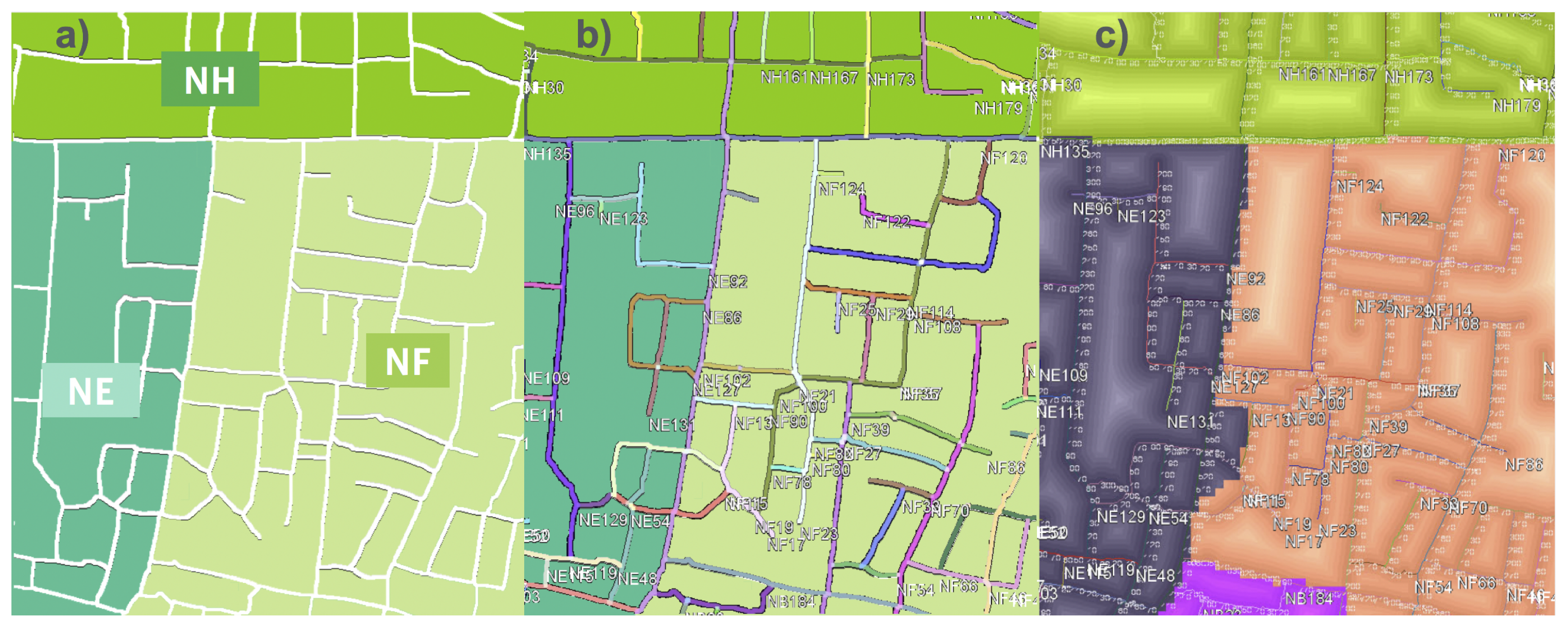
After we gather all clustered segments from the segmentation phase, we start by labeling the regions on the basis of proximity and orientation. We compute the most dense region by a simple metric of the average number of roads per unit area, and we name this region “CA” for the city center. We divide all other regions into four categories on the basis of where the region midpoint is located with respect to the city center: N(orth), S(outh), W(est), and E(ast). Next, we trace the adjacent regions in each bucket, on the basis of their distance from the city center, and assign letters in that specific order, following the spiral pattern of the London post code system. For example, the regions at the north of the center would be named NA, NB, NC, and so on. Figure 8a shows three such example regions, NE, NF, and NH.
Naming the regions allows us to start naming the roads. The roads in each region are divided into two groups on the basis of their two main directions. We need such directionality to decide on the parity of the road name: odd for north–south bound, and even for east–west bound. We use a similar orientation bucketing approach to decide the dominant orientations. If a road does not belong to either of the two main directions, it is approximated to the closest. The main direction is assigned odd parity, and the second main orientation (in most cases perpendicular to the main orientation) is assigned even parity. Then the road segments are numbered according to their order. Figure 8b demonstrates the roads named following the design requirements mentioned in Section 3.
Labeled roads enable us to proceed to the last stage: house labeling. For each road segment, we place a virtual meter marker every 5 m (calculated in Euclidian pixel space). We distinguish the structures on the left and right sides of the roads by even and odd numbering. On the basis of the right-hand rule from the starting point of a road segment, we name the addresses on the right as even and on the left as odd (noting that the neighbors across a street at the same meter marker will have consecutive numbers, even and odd). We also compute a distance field of the roads and discretize that field by a 5 m step size. Every band of the distance field is assigned a block letter, concluding the address generation. We use the discretized orthogonal distances and meter markers as an oriented x- and y-axis and decide the house number of a point accordingly. The distance computation in all cases is approximated by the pixel neighborhood: 4-neighborhood pixels are incremented by 1 and 8-neighborhood pixels are incremented by 1.4. Finally, Figure 8c depicts the meter markers along the labeled roads, and the gradient towards the roads represents the block letters.

4.5. Output Formats

Finally, we vectorize our road and region maps to export in OSM format, by converting the pixels into nodes with latitude and longitude, with their relative meter marker distance encoded as an attribute. Moreover, we output .json files for encoding per pixel the house naming information. Being a generative map, it is not possible to store all the per-pixel information beforehand; thus we only encode the road network and leave the first field of the address format to be computed and generated on the fly, whereas the other fields are precomputed and stored for efficient querying.
Instead of encoding all nodes, another alternative output format is shape files. The street-aligned grid-like boxes are encoded as polygons in shape files indexed by city names. The files are not to exceed 2 GB, and they hierarchically encode regions. We note that although we call them street-aligned grids, the cells are not necessarily shaped as rectangles, as they are based on the intersection of distance field curves formed along and perpendicular to the roads.

5. Inaccessible Areas

Putting streets in focus creates a drawback for geocoding structures that are considerably further from any street. Our design specifications dictate a scheme that is globally applicable; thus we wanted to extend our format to cover areas that are not accessible by streets. We have explored different implementations to cover such areas, which are 26 × 5 m away from any street.
We formulate geocoding as a function f ( l a t , l o n ) = w , with different knowns and unknowns, converting to our scheme as f ( ? ) = x . y . z . t (excluding the version field). For places with roads, it is assumed that the function is fed with the road network R, the city, and the country information C. Thus, we can express the parameter space as f ( R , C ) = x . y . c i t y . c o u n t r y . However it may be the case that the point to be geocoded is not in the range of the distance fields, is not accessible by a street, or is not in a city, in the extreme case (i.e., the coordinates of a ship in the Atlantic Ocean). Even in these cases, the information should be presented in the same format. In this case, the road, city and country information will be nullified, up to the level that the only reliable information remains as the latitude/longitude pair for that particular point. Thus the true parameter domain can be represented as f ( R + , C + , ( l a t , l o n ) * ) = x . y . z . t , where + means 0 or 1, and ∗ means valid only if others are nullified.

5.1. Linear Hashing

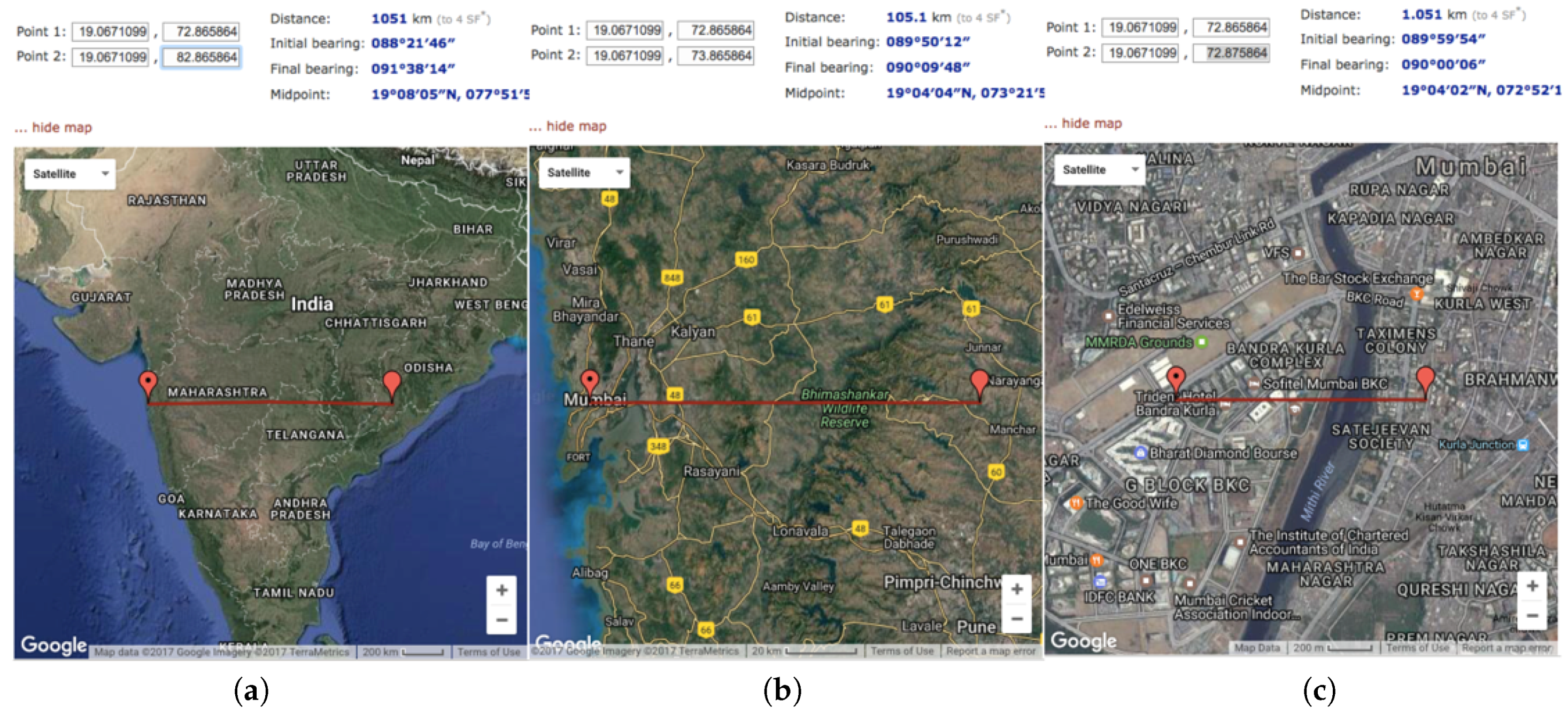
In order to convert the known information into unknown information, we propose a hierarchical hashing of spatial coordinates. For this scheme, we choose a precision of 100 m × 100 m, using the three floating-point information elements in latitude and longitude. This is chosen with the assumption that while we do not want our system to return a null value for such areas, for the current system to span the “blackholes”, it is efficient enough to work with a coarser spatial approximation. Figure 9 shows the relation of the coordinate approximation and granularity of address cells.
The task reduces to converting the latitude/longitude pairs (each of which could be as long as 12 characters, including a sign character, at the highest precision) to fit into 10 characters, and we try to ensure that the design principles of the address format still hold, meaning that some portion of those 10 characters are hierarchical, linear and cognitively traceable. To decide on the alphanumeric format, we explored 26 letters of the alphabet and 10 digits, totaling up to 36 characters. Base 36 becomes the hash function, as we have a total of 36 characters at our disposal. Converting the range 359.999 (without the floating point) to base 36, we obtain “7PRZ”. Thus the complete address for the longitude block would be 7PRZW, where the fourth character stands for the hemisphere. The same procedure can also be applied to latitudes, so that the full notation for f ( C , ( l a t , l o n ) ) = h a s h ( r o u n d ( l a t , 3 ) ) + d i r ( l a t ) . h a s h ( r o u n d ( l o n , 3 ) ) + d i r ( l o n ) . C is L-A-T-dir.L-O-N-dir.name.Ocean/Continent/etc. The Atlantic Ocean case becomes H3TRW.3EWGS.ATLNC.OCEAN.

5.2. Hierarchical Hashing

Up to here, the proposed scheme is only linear, not hierarchical. Namely, spatially adjacent addresses may not have consecutive names (359.999 named as 7PRZW and 360.000 named as 7PS0W); hierarchically different addresses do have consecutive names (two structures across the city border may have consecutive names, independently of their relative distances to their city centers). To overcome this issue, we have designed hierarchical hashing. We decrease the accuracy of linear hashing by enlarging the grid from 100 m × 100 m to 1 km × 1 km, using two floating points of the coordinates, instead of three. This provides three letters of the new address. Within each 1 km × 1 km cell of three letters, we relatively re-hash it to a 36 × 36 grid, with an additional letter. The new address cells end up with a resolution of 30 m, represented by five letters: the first level hash (3), second level hash (1) and the direction (south/north or east/west). A similar scheme is proposed by plus codes [3]; however the design choices of linearity and hierarchy are more convoluted in this format (i.e., random letter grids with no linear ordering). If we express it in our geocoding formulation, it becomes f ( C , ( l a t , l o n ) ) = h a s h ( r o u n d ( l a t , 2 ) ) + h a s h ( l a t - r o u n d ( l a t , 2 ) ) + d i r ( l a t ) . h a s h ( r o u n d ( l o n , 2 ) ) + h a s h ( l o n - r o u n d ( l o n , 2 ) ) + d i r ( l o n ) . C , which is expressed as L l a t L l a t H l a t D l a t . L l o n L l o n H l o n D l o n . n a m e . O c e a n / C o n t i n e n t / e t c .

6. Results and Applications

Our system is written in Python and C++ and is not multi-threaded; the implementation is on the CPU (except the road extraction part, which runs on 8+ GPUs). We use the Chainer [50] implementation skeleton for all the neural network models and use networkx and sci-kit libraries for some clustering algorithms. We have developed an automatic pipeline to process any satellite imagery, and we used our approach to process more than 10 cities, totaling up to more than 16 K km 2 . Except the learning part, the system is O ( n ) , where n is the number of road pixels in an upsampled image, or the number of road segments for region creation. We compare our intermediate outputs and resulting maps to ground truth and other available maps in different stages. We also share our preliminary results for improving travel times on the basis of user experience with the new addressing format. Finally, the source code to convert .osm files and geotiffs to street addresses is available on our repository (https://github.com/facebookresearch/street-addresses).
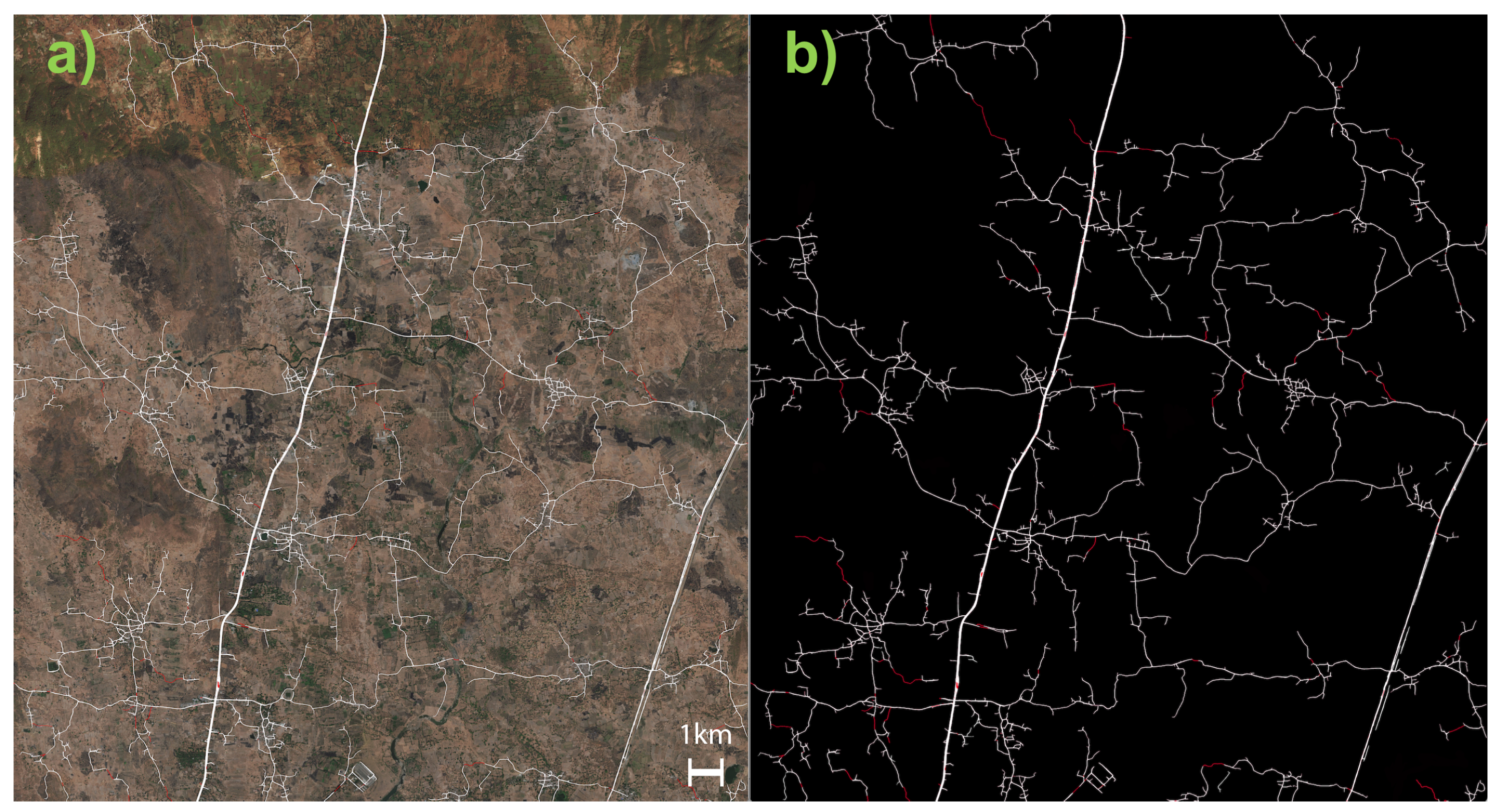
Similarly to the preparation of the training data, we created binary road masks from additional tiles of unmapped areas as ground truth and consolidated these together with our road extraction results (before finding individual road segments). Figure 10 shows the comparison with ground truth for the extracted roads of an unmapped suburban area. Our SegNet model and post-processing approach were able to learn 90.51% of the roads (white), and the missing parts are colored in red. This success ratio (defined by the ratio of manual corrections) was close to 80% on average per city, increasing in more structured urban environments.
We demonstrate intermediate results of our algorithm in a traditional U.S. city that is already well mapped. We have compared street segments dictated by the traditional addresses and our generative addresses (Figure 11). Comparing the road segments, we accomplished extracting 95% of the roads (i.e., the ratio of overlapping road pixels over all the road pixels present in the rastered map) in that particular city tile. Comparing the addresses, we also observed that although traditional addresses are more established by the people and the culture, our addresses are easier to remember and support intuitive self-location and navigation.
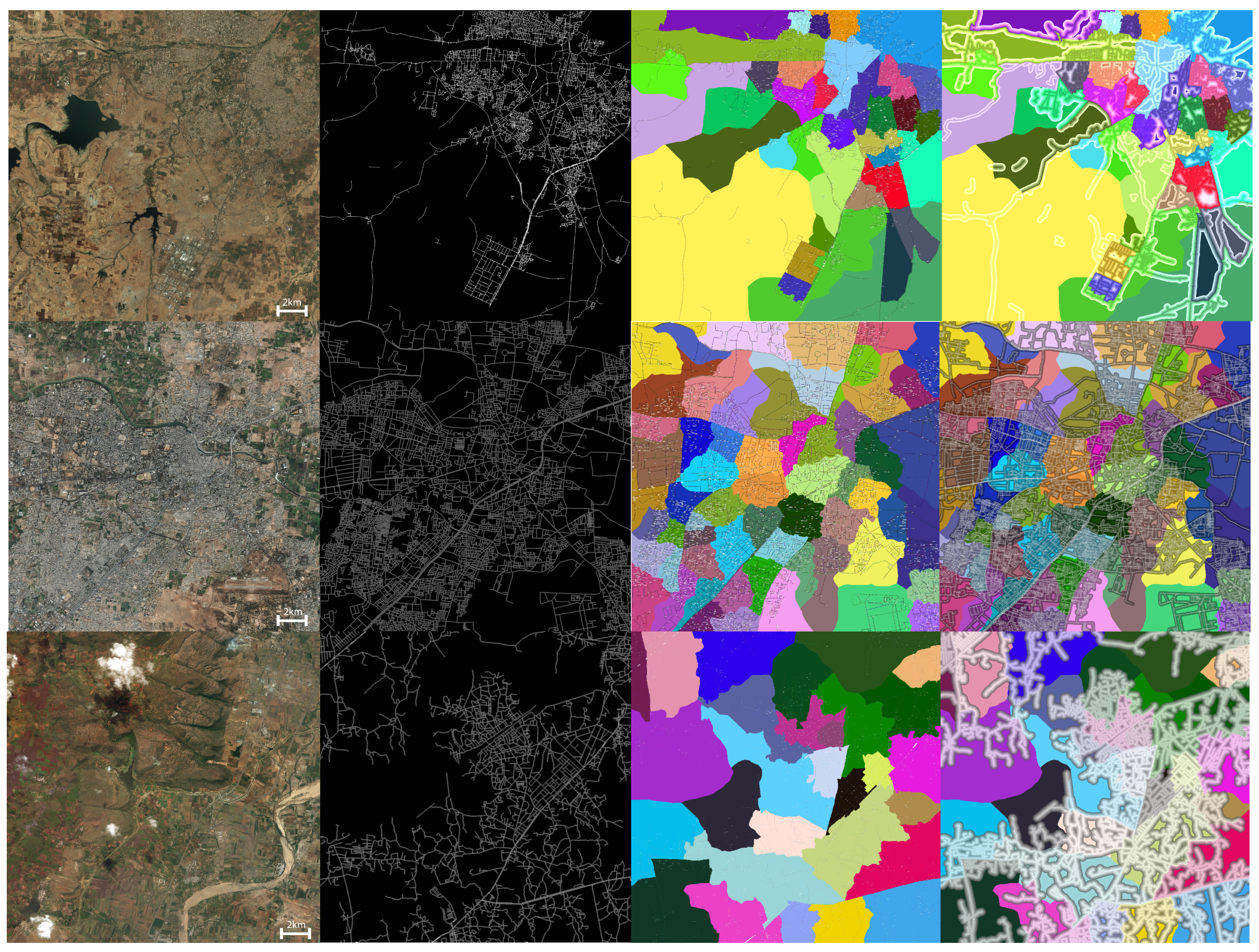
However, keeping the motivation of providing street addresses to the approximately 4 billion unconnected people, our results in fact shine for developing countries, where the structure of the road network is less grid-like. Figure 12 shows our generative maps in the same format, on three different cities in unmapped developing countries. We accomplished automatically addressing more than 80% of the populated areas, which significantly improved the current map coverage in those areas. We also demonstrate the relevant population characteristics of the cities in Table 1. The population estimates are presented per tile and are taken from various recent government census databases. The population density information is presented per city and is taken from Wikipedia.
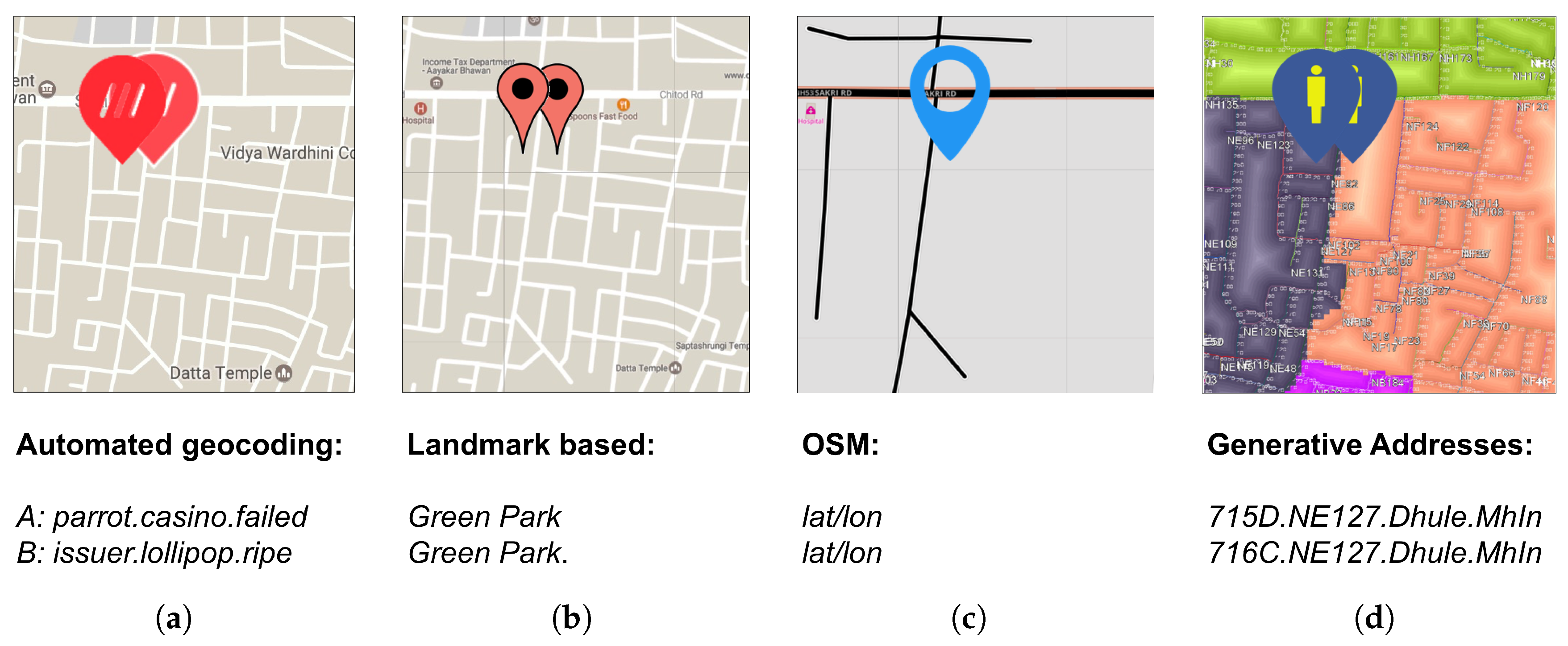
We also show how we bridge the gap between traditional addresses and geocodes, as well as increased map coverage. Our design principles (Section 3.1) allow us to use advantages of both, and all are easily convertible to each other. Furthermore, being an automatic system, based on human-built structures on the ground, we neither need human authorities to map an area nor need to map deserted areas such as geocodes. We have compared our maps to other popular addressing solutions in Figure 13. For the same point on earth, [1] contains some unlabeled roads and outputs three random words parrot.failed.casino as the address. Google Maps also contains some roads around this point; however because such places are unmapped, it outputs Green Park on the basis of the landmark, for a couple of kilometers around the point. OSM, on the other hand, does not even contain the roads, and the point can be reached only by its latitude and longitude. However, our generative maps extract the roads almost completely and assign a unique address to the point as 715D.NE127.Dhule.MhIn. Overall we improve the semantic relations of addresses compared to [1]. For our test region, our contribution is even more visible for the true street names; we have increased the addresses compared to Google Maps (by comparing labeled vs unlabeled road geometry) and achieved almost 100% overall coverage compared to OSM (by comparing aligned maps).
We have evaluated the usefulness of our generative maps with some treasure hunt-like user experiences. We compared the travel times using the old and new addressing schemes. We invited several local people with a low education level for a self-navigation game using our addresses. The participants were local enough to know their environment, but their neighborhood had no structured addresses (i.e., landmark-based system of lengthy descriptions). For data collection with old addresses, given the traditional address of the location, we simply tracked the users with GPS devices to collect their trails. They also clicked a button when they started a new trail and when they found the address (so that we refrained ourselves from the time spent on the puzzles and other factors). For data collection with new addresses, we first converted the places of interest with old addresses to a new addressing format. Then we printed a map of the area that we generated and gave a small tutorial to the users about how to read our map (i.e., a brief introduction, as in Section 3). Afterwards, they followed the same procedure and the same (or more efficient) trails, following our map. Some example trails and the corresponding travel times are shown in Figure 14. The travel times with new addresses are plotted in blue, old addresses are plotted in orange, and the difference is shown in gray, with confidence intervals in green. We note that overall, the travel times decreased by 21.7%, with our system producing a 52.4 s improvement on average and decreasing the last mile of activity (which included asking around the exact building), proving the accuracy of our addresses. Although the crowd should have had a positive bias for traditional addresses, the linear and hierarchical structure of our addresses helped them to find the location more intuitively. There were also some incidents based on external variables such as traffic and animal interruptions for some trails. These were not filtered, as they were not properly reported; however extreme cases (such as a 10 m difference) were interpreted as the consequences of such external problems.
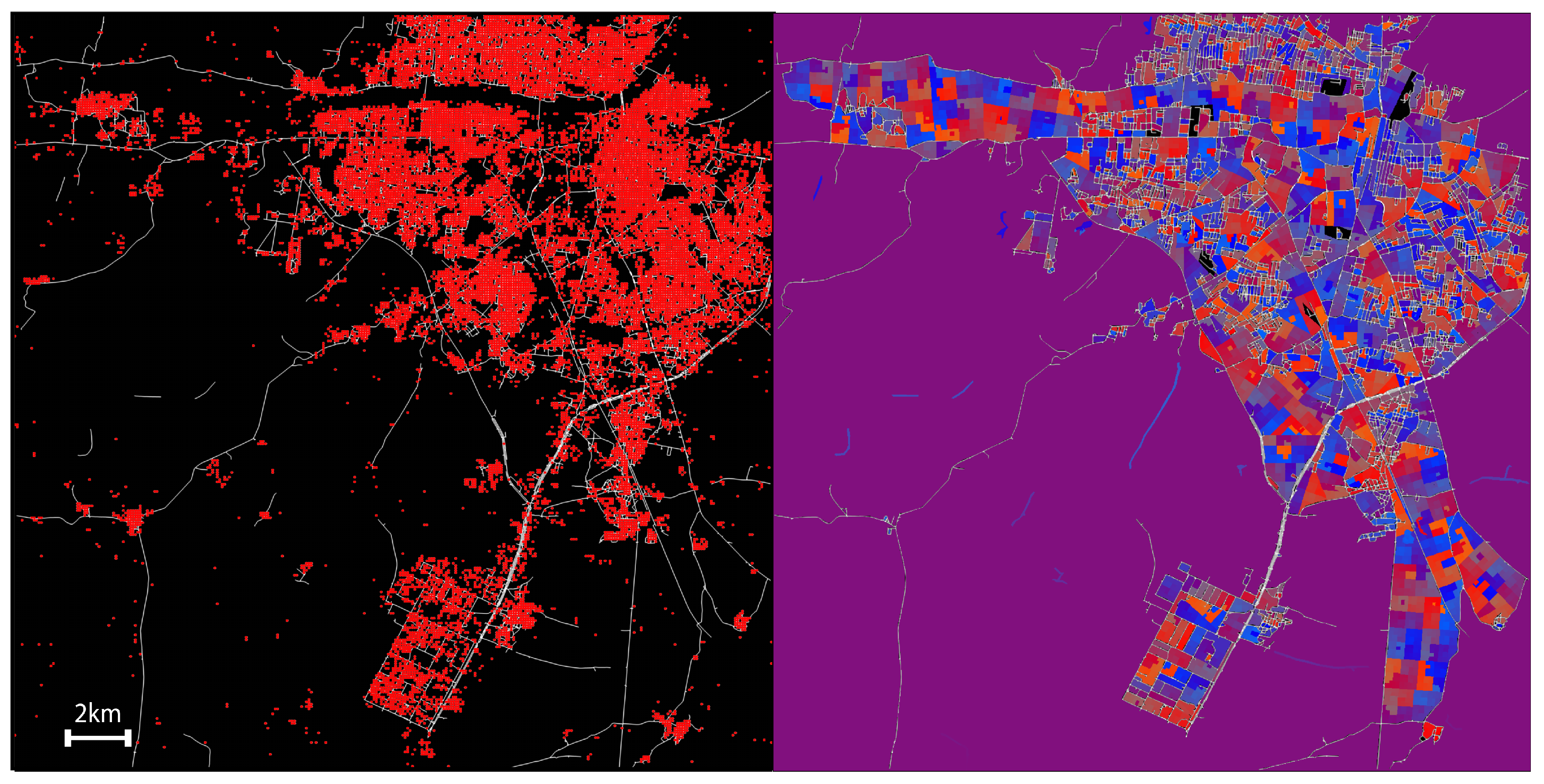
We used population density data [4] to evaluate how our algorithm reflects density criteria, as demonstrated in an example tile in Figure 16(Left), discussed in Section 8. The evaluation criteria include the number of assigned cells aligned along the road and a penalty of building road overlap. The results of the first experiments indicated that our addresses are coherent with the population density.

7. Extensions and Discussion

We have deployed our system in small use cases for various users and discovered a number of ways to strengthen our approach. First of all, we start with a theoretical analysis for the determinism of separate steps of our approach, followed by a practical implementation of an address server and our solutions for edge cases.

7.1. Determinism, Repeatability, and Complexity Analysis

We look at the determinism of each step of our algorithm and investigate the assumptions to ensure determinism. This analysis is needed to assess the consistency between multiple runs of the algorithm. Although we store the generated addresses in a place name server (PNS) Section 7.2, we would like to update our database every year, and this analysis ensures that multiple runs converge on similar maps.
Road Geometry: Once the model is trained using the particular subset of an area, it is assumed to perform reasonably well within that particular area. If the performance is below the standard, then we train a new network with an improved subset. Although it would be incorrect for this to be concluded as deterministic for a deep learning approach, we at least enforce the performance criteria as a measure for determinism; thus predictions of a satellite images will always produce proper roads.
The deep learning models introduced in Section 4.2 work on multiple GPUs and converge from a couple of hours up to a day on the basis of the epoch. We have concluded that the SegNet model converges faster (50 epochs with 65% less time). We also converted our models to Caffe2 from chainer and enabled distributed training, so that the training time is limited to a few hours at most. The prediction step takes 1–2 min per a 400 km 2 tile, which is not significant compared to the training time.
Regions: Although being probabilistic in nature, the normalized min-cut algorithm to partition the graph converges to the same output in multiple runs. In this way, the region algorithm is deterministic given a particular road geometry (but not deterministic given only a city, carrying the nondeterminism of the previous step of road prediction). Next, the regions are named. Given a city center as the seed and regions from the previous step, the name given to a particular region will be based on the distance-based spatial ordering from the city center. Because the ordering will be the same, the names will be the same at every run of the algorithm. Additionally, even if the regions are slightly different, it is likely that they will receive the same name, given that the number of regions and the cluster means will be similar.
For the complexity of creating regions, normalized min-cut requires O ( n 3 ) , where n is equal to the number of road segments. However, we calculated the adjacency matrix of the roads, which ends up being a very sparse matrix; thus, the O ( n ) variant is used for our algorithm. For the Newman–Girvan algorithm, this is quite the opposite, because the sparser the structure becomes, the more communities that emerge, in which case, the algorithm converges to its worst case scenario of O ( m 2 n ) . This is one of the practical behaviors that we have observed in Section 4.3. The rest of the naming and labeling work on sequential lists of regions and roads, which is O ( n ) (the ordering is neglected because it either comes from constant spatial queries or from the previous step).
Labeling: Given the regions, names, and roads, the code to name the roads is deterministic. The roads are named with a concatenation of the region label and road number, which is increasing and even for the north/south orientation and increasing and odd for the east/west orientation. Lastly, we determine the 2D distance of a queried point according to the nearest road, assuming that the coordinate system is aligned with the nearest road. The distance along the road axis becomes the meter marker number, and the distance along the perpendicular axis becomes the block letter. Because all namings are only distance queries, this step is also deterministic.
All the sequential labeling and distance queries require constant time; thus this step takes O ( m ) time overall, where m is the number of address cells. Our PNS implementation leaves this last step as an on-the-fly computation; thus we address per query (instead of addressing the whole world and storing for every 3×3 cell).
Overall: Finally, we can conclude that the determinism of the overall algorithm depends on the road predictions. We enforce the performance criteria for the learning part, and the city center extraction is automated on the basis of the density of regions; thus the overall algorithm is deterministic within an epsilon of the performance criteria of the road graph extraction.
The most computationally resource-dependent step is the deep learning part, as expected. However we have reduced this time by distributed multi-GPU implementation. Afterwards, the region creation is made more efficient by a sparse matrix implementation, running linearly on the basis of the number of roads. The rest of the algorithm is not computationally intensive.

7.2. A Global Address Space: Place Name Server

Because it is a nondeterministic algorithm overall (because of the deep learning prediction stage), and because it would be inefficient to generate addresses from scratch for each use case, we have decided upon storing all generated addresses in a database for easy forward/reverse spatial querying. We call this database the PNS: a domain name server (DNS)-like system for forward and reverse geocoding via a REST API. All addresses are encoded in an efficient, robust, and flexible format. The encoding is stored in an efficient database, is supported by a scalable and optimized API—allowing millions of reads per day—and is extendible to respond to future needs, such as sub-delegation for content manipulation.
The PNS is derived by following the principles of a DNS; thus we first revisit the DNS structure. DNSs were created to maintain a directory of domain names and translate them to Internet Protocol (IP) addresses. The DNS exhibits a hierarchical namespace, implemented as a distributed database structure in which sub-namespaces can be delegated to trusted parties. The DNS provides semantic names (DNS addresses) to location-dependent IP addresses (location in the network). This is necessary because, although domain names are easy for people to remember, machines access Web sites on the basis of IP addresses. Similarly, street addresses provide semantic names to geocoordinates. Street names and business addresses should be easy for people to remember. A machine will be able to access locations on the basis of latitude and longitude. The DNS is attractive for two main reasons: (i) it allows global scaling via name-space delegation; and (ii) it has a very lightweight query/response protocol.
The street address needs to be encoded as a string (in PNS format), e.w. N13455.W12345.reverse.geo, asking for latitude/longitude to be mapped to a most appropriate name. First, the string-encoded latitude/longitude pair passes as a name in the question section. Second, the server attempts to find the closest matching name. Third, the server responds with a PTR resource record pointing toward the geoname or signifies an error. We note the above takes only one round-trip, and the server attempts to find closest name using some internal logic. Potentially, one may encode a radius in the name, for example, N13455.W12345.R100.approx.reverse.geo, asking for all names within 100 m of the specified latitude/longitude location. In this case, the server would return multiple PTR records, one for each name found within the radius of the specified location. The number of names returned may be too large to fit into the response. In this case, the response would indicate truncation.
The current database structure has two tables, which are roughly analogous to OSM’s standard relational database structure and Overpass’s spatial database. The first of these tables is primarily for converting our addresses to latitude/longitude pairs (forward-geocoding). The second is for reverse-geocoding. In the case of forward-geocoding, we wish to turn 110B.NC17.MPK.USA into some geospatial coordinates; 110B is computed after determining the road, but the other three fields will each be given by a table.
The table for reverse-geocoding instead stores edges in coordinates along with a spatial index to allow bounding-box queries. When a coordinate is searched, the table is queried for the corresponding bounding box. Then the returned edges are compared against the given latitude and longitude to find the nearest. When we have the nearest point, we obtain the road, city, and country from the tables. We then compute the first address block using the edge coordinate and the distance.

7.3. Other Extensions

7.3.1. Versioning and Updates

Although we store the generated addresses in a database, the living space in the world keeps growing, and we need to update our database (and consequently the addresses) in time. We have chosen to add versioning as an extension to the current system, as the last field indicating the year that the address is generated.
However, during the year, if new roads are built on the ground, there should be updates to the addresses. In order to prevent changing the names of existing roads before the yearly update, we implement in-between addresses. These addresses follow the same format but are one level deeper in the hierarchy relative to the existing addresses. As an instance, if a new road is detected between WK15 and WK17, we would match the previous roads, and the new road is assigned a new name, WK15a, to indicate that it is between WK15 and the next road.
If the urban structure of a city is significantly changing such that new regions emerge, then we assign new names to the regions without changing the old region names. We note that this happens in extreme cases, such as adding (or deleting) 300 or more road segments in an approximately 5 km × 5 km area. In this case, we do not change the structure of the existing regions, but we give a new name to the region with emerging roads, following the same in-betweenness convention (i.e., NC is divided into NC (old roads) and NCa (new roads)).

7.3.2. Missing City Boundaries

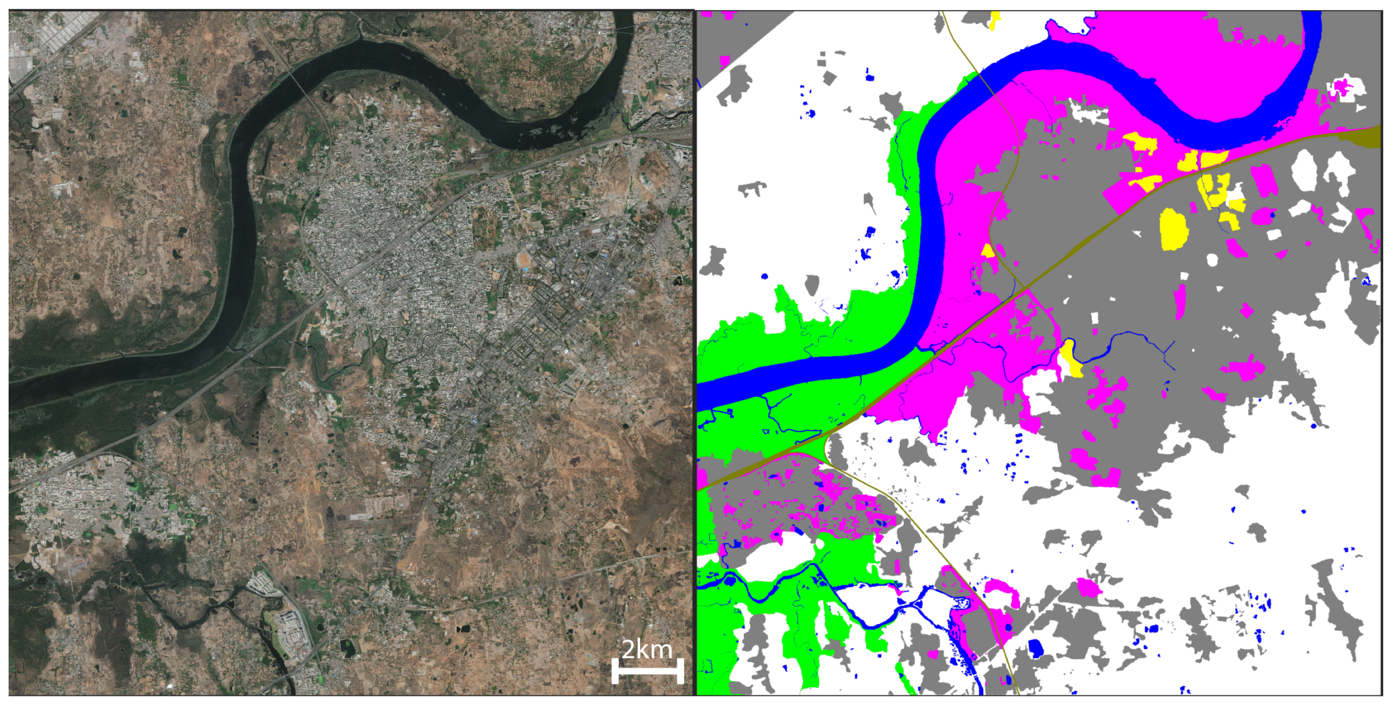
After querying OSM and other available open datasets, if there is no city boundary information for a particular area, we use a land cover classification model. We assume that if there is no open data source for a city, the city lies in a developing area, such that the visual inspection of city boundaries from satellite imagery is possible. The model is trained on the same input satellite images with class labels for nine different land types (urban, forest, water, grass, farm, mountain, land, cloud, and unknown). The network is similar in layers to the road segmentation model; however we tweak the last layer for multi-class segmentation. Then the area is partitioned into the main types, and the partitions are processed to obtain city masks to create the regions of interest. Figure 15 contains an example tile labeled with such main land cover types.

7.3.3. Overflowing Regions

This is the inverse problem for inaccessible areas: what if a city is too dense? For cities that are dense enough (300 roads/region * 26 region/orientation * 4 orientations + 1 downtown = 30 k roads in a city), we introduce an extension scheme to map in eight main directions instead of four directions, which include the diagonal directions (SW, SE, NE and NW) after a threshold radius is reached. We name these regions as P, Q, R and T in addition to N, S, E and W, being memorable letters not easily confused.

7.3.4. Roads in 3D

For some rare urban scenarios, we have observed that some cities may contain stacked highways and double roads. In such cases, generally one of the roads overlapping in the z direction is a highway. However, it is traditionally more convenient to address the surrounding areas according to the non-highway road. To encode this rule, we store the existing road tags in the OSM querying phase. Later, when there are multiple closest streets for a given point, we use these tags to decide on which road a point lies.

8. Limitations and Future Work

As a supervised learning approach, our algorithm is sensitive against errors in the training data; that is, the ground truth segmentation may be fundamentally wrong or disconnected. However, we have experimentally observed that our learning model is deep enough to support training on more data. As a consequence, as we added more diverse cases (i.e., more countries) to our training data, we were able to handle such cases more accurately. Employing other data sources (population distribution, user trails, etc.) can also improve the prediction accuracy. Datasets such as that in Figure 16(Left) can be used for both the evaluation of dense predictions and the enhancement of sparse predictions.
Because the region concept is not well defined enough to be mathematically formulated, we intend to validate our regions by first establishing a metric similar to the maps’ validation and also employ human annotators to validate qualitatively the presence of significant differences among regions. Our domain experts have helped us to enumerate some criteria (borrowed from the urban planning world) to evaluate our regions; however we would like to mathematically formulate these rules to evaluate our regions numerically. Our first attempt for such an evaluation is depicted in Figure 15 as the land cover classification. We would like to measure the accuracy of our regions by their overlap with the boundaries of different land types predicted by our network.
The last future work item that we have run experiments on is to convert the meter marker logic to a state-of-the-art parcel subdivision method [8]. The constraint subdivision divides the blocks into parcels, which obey the road topology and follow some constraints, such as having adequate street access, being of approximately the same sizes, having less split irregularity between them, and so forth. The first optimized experiment is shown in Figure 16(Right). We believe that instead of simple proximity queries, smart subdivision is needed to respond to real urban planning scenarios of both developing and future cities.

9. Conclusions

Overall, we have presented a generative system that can be applied to any given mapped or unmapped area, producing a complete street labeling solution. Improved street labels will improve the map coverage and physically connect the people to the economy, as well as help to provide aid in disaster zones. Connecting the unconnected should increase the economic, juridical, and life-sustaining involvement of people all around the world. It improves the outreach of businesses and the economy, as well as the accuracy and efficiency of providing first aid in disaster zones.
To accomplish our aims, we have introduced an addressing scheme and a full system to generate addresses coherent with road topology. Our approach merges state-of-the-art deep learning and computer vision techniques to detect roads and regions from satellite images. We then perform labeling of such urban elements to provide accurate, topological, and intuitive addresses. In future, we would like to scale up and enable large entities such as states or cities to adopt our addressing system.

Acknowledgments

We would like to thank all team members for their tremendous efforts in the project, namely, Divyaa Ravichandran, Kleovoulos Tsourides, Amandeep Bal, Mohamed Alaoudi, Guan Pang, and Jing Huang. We would like to thank Harshita Shrivastva, Richi Raut, and Jatin Malhotra for the data collection. We would also like to thank Saikat Basu and Ming Gao for their insights. We also wish to acknowledge Manohar Paluri, Pierre Roux, Ryan Peterson, Yael Maguire and Baris Erkmen for their support.

Author Contributions

Ramesh Raskar provided the core idea of ‘Street Addresses for All’ research and helped to mature the design as the leader of the team. All authors contributed into the design and implementation of the project. Aman Raj and Forest Hughes performed machine learning experiments for road extraction and region creation. Kaunil Dhruv implemented the infrastructure and the backend. Sanyam Garg and Surya Muddala performed the data analysis. Ilke Demir designed experimental validations and evaluations, performed the theoretical analysis, and wrote the manuscript. Ilke Demir, Forest Hughes, and Barrett Doo contributed to the extensions of the system. Barrett Doo coordinated the efforts.

Conflicts of Interest

The authors declare no conflict of interest.

References

  1. Jones, G.R. Human Friendly Coordinates. GeoInformatics 2015, 18, 10–12. [Google Scholar]
  2. OpenStreetMap. Haiti Project. 2011. Available online: https://hotosm.org/projects/haiti-2 (accessed on 11 December 2017).
  3. Open Location Code: An Open Source Standard for Addresses, Independent of Building Numbers and Street Names. Available online: https://github.com/google/open-location-code/blob/master/docs/olc_definition.adoc (accessed on 1 December 2017).
  4. Zhang, A.; Gros, A.; Tiecke, T.; Liu, X. Population Density Estimation with Deconvolutional Neural Networks. In Proceedings of the Workshop on Large Scale Computer Vision at NIPS, Barcelona, Spain, 5–10 December 2016. [Google Scholar]
  5. Demir, I.; Hughes, F.; Raj, A.; Tsourides, K.; Ravichandran, D.; Murthy, S.; Dhruv, K.; Garg, S.; Malhotra, J.; Doo, B.; Kermani, G.; Raskar, R. Robocodes: Towards Generative Street Addresses from Satellite Imagery. In Proceedings of the IEEE International Conference on Computer Vision and Pattern Recognition Workshops, Honolulu, HI, USA, 21–26 July 2017. [Google Scholar]
  6. What Is the Right Addressing Scheme for India? Available online: http://mitemergingworlds.com/blog/2017/11/22/what-is-the-right-addressing-scheme-for-india (accessed on 1 December 2017).
  7. Chen, G.; Esch, G.; Wonka, P.; Müller, P.; Zhang, E. Interactive Procedural Street Modeling. ACM Trans. Graph. 2008, 27, 103. [Google Scholar] [CrossRef]
  8. Vanegas, C.A.; Kelly, T.; Weber, B.; Halatsch, J.; Aliaga, D.G.; Muller, P. Procedural Generation of Parcels in Urban Modeling. Comput. Graph. Forum 2012, 31, 681–690. [Google Scholar] [CrossRef]
  9. Parish, Y.I.H.; Müller, P. Procedural Modeling of Cities. In Proceedings of the 28th Annual Conference on Computer Graphics and Interactive Techniques (SIGGRAPH ’01), Los Angeles, CA, USA, 12–17 August 2001; ACM: New York, NY, USA, 2001; pp. 301–308. [Google Scholar]
  10. Aliaga, D.G.; Vanegas, C.A.; Benes, B. Interactive Example-based Urban Layout Synthesis. ACM Trans. Graph. 2008, 27, 160. [Google Scholar] [CrossRef]
  11. Sun, J.; Yu, X.; Baciu, G.; Green, M. Template-based Generation of Road Networks for Virtual City Modeling. In Proceedings of the ACM Symposium on Virtual Reality Software and Technology (VRST ’02), Hong Kong, China, 11–13 November 2002; ACM: New York, NY, USA, 2002; pp. 33–40. [Google Scholar]
  12. Aliaga, D.G.; Demir, I.; Benes, B.; Wand, M. Inverse Procedural Modeling of 3D Models for Virtual Worlds. In Proceedings of the ACM SIGGRAPH 2016 Courses (SIGGRAPH ’16), Anaheim, CA, USA, 24–28 July 2016; ACM: New York, NY, USA, 2016; p. 16. [Google Scholar]
  13. Wang, Y.; Liu, X.; Wei, H.; Forman, G.; Zhu, Y. CrowdAtlas: Self-updating Maps for Cloud and Personal Use. In Proceedings of the 11th Annual International Conference on Mobile Systems, Applications, and Services (MobiSys ’13), Taipei, Taiwan, 25–28 June 2013; ACM: New York, NY, USA, 2013; pp. 469–470. [Google Scholar]
  14. Skoumas, G.; Pfoser, D.; Kyrillidis, A.; Sellis, T. Location Estimation Using Crowdsourced Spatial Relations. ACM Trans. Spat. Algorithms Syst. 2016, 2, 5. [Google Scholar] [CrossRef]
  15. Mattyus, G.; Wang, S.; Fidler, S.; Urtasun, R. Enhancing Road Maps by Parsing Aerial Images around the World. In Proceedings of the 2015 IEEE International Conference on Computer Vision (ICCV), Santiago, Chile, 7–13 December 2015; pp. 1689–1697. [Google Scholar]
  16. Mattyus, G.; Luo, W.; Urtasun, R. DeepRoadMapper: Extracting Road Topology from Aerial Images. In Proceedings of the IEEE International Conference on Computer Vision (ICCV), Venice, Italy, 22–29 October 2017. [Google Scholar]
  17. Zeng, D.; Zhang, T.; Fang, R.; Shen, W.; Tian, Q. Neighborhood geometry based feature matching for geostationary satellite remote sensing image. Neurocomputing 2017, 236, 65–72. [Google Scholar] [CrossRef]
  18. Wang, J.; Song, J.; Chen, M.; Yang, Z. Road network extraction: A neural-dynamic framework based on deep learning and a finite state machine. Int. J. Remote Sens. 2015, 36, 3144–3169. [Google Scholar] [CrossRef]
  19. Zhao, J.; You, S. Road network extraction from airborne LiDAR data using scene context. In Proceedings of the 2012 IEEE Computer Society Conference on Computer Vision and Pattern Recognition Workshops, Providence, RI, USA, 16–21 June 2012; pp. 9–16. [Google Scholar]
  20. Li, P.; Zang, Y.; Wang, C.; Li, J.; Cheng, M.; Luo, L.; Yu, Y. Road network extraction via deep learning and line integral convolution. In Proceedings of the 2016 IEEE International Geoscience and Remote Sensing Symposium (IGARSS), Beijing, China, 10–15 July 2016; pp. 1599–1602. [Google Scholar]
  21. Xu, L.; Jun, T.; Xiang, Y.; JianJie, C.; LiQian, G. The rapid method for road extraction from high-resolution satellite images based on USM algorithm. In Proceedings of the 2012 International Conference on Image Analysis and Signal Processing, Hangzhou, China, 9–11 November 2012; pp. 1–6. [Google Scholar]
  22. Peteri, R.; Celle, J.; Ranchin, T. Detection and extraction of road networks from high resolution satellite images. In Proceedings of the 2003 International Conference on Image Processing, Barcelona, Spain, 14–17 September 2003; Volume 1. [Google Scholar] [CrossRef]
  23. Poullis, C.; You, S.; Neumann, U. A Vision-Based System For Automatic Detection and Extraction of Road Networks. In Proceedings of the 2008 IEEE Workshop on Applications of Computer Vision, Copper Mountain, CO, USA, 7–9 January 2008; pp. 1–8. [Google Scholar]
  24. Wegner, J.D.; Montoya-Zegarra, J.A.; Schindler, K. A Higher-Order CRF Model for Road Network Extraction. In Proceedings of the 2013 IEEE Conference on Computer Vision and Pattern Recognition, Portland, OR, USA, 23–28 June 2013; pp. 1698–1705. [Google Scholar]
  25. Alshehhi, R.; Marpu, P.R. Hierarchical graph-based segmentation for extracting road networks from high-resolution satellite images. ISPRS J. Photogramm. Remote Sens. 2017, 126, 245–260. [Google Scholar] [CrossRef]
  26. Anwar, T.; Liu, C.; Vu, H.L.; Leckie, C. Partitioning road networks using density peak graphs: Efficiency vs. accuracy. Inf. Syst. 2017, 64, 22–40. [Google Scholar] [CrossRef]
  27. An Entire Village Gets Street Names. 2016. Available online: http://mitemergingworlds.com/blog/2016/8/14/an-entire-village-gets-street-names (accessed on 1 December 2017).
  28. Economic Impact of Discoverability. 2018. Available online: http://mitemergingworlds.com/blog/2018/2/12/economic-impact-of-discoverability-of-localities-and-addresses-in-india (accessed on 15 February 2018).
  29. Tian, Q.; Ren, F.; Hu, T.; Liu, J.; Li, R.; Du, Q. Using an Optimized Chinese Address Matching Method to Develop a Geocoding Service: A Case Study of Shenzhen, China. ISPRS Int. J. Geo-Inf. 2016, 5, 65. [Google Scholar] [CrossRef]
  30. Weihong, L.; Ao, Z.; Kan, D. An Efficient Bayesian Framework Based Place Name Segmentation Algorithm for Geocoding System. In Proceedings of the 2014 Fifth International Conference on Intelligent Systems Design and Engineering Applications, Zhangjiajie, Hunan, China, 15–16 June 2014; pp. 141–144. [Google Scholar]
  31. The City of London. London Postal Code System. 2016. Available online: https://www.london.gov.uk/sites/default/files/gla_postcode_map_a3_map1.pdf (accessed on 1 December 2017).
  32. London Postal Codes. Available online: https://www.doogal.co.uk/londonpostcodes.php (accessed on 1 December 2017).
  33. Ministry of the Interior and Safety—Map Services. Available online: http://www.juso.go.kr/support/AddressMainSearch2.do (accessed on 1 December 2017).
  34. Berliner Hausnummern. Available online: https://hausnummern.tagesspiegel.de (accessed on 1 December 2017).
  35. Farvacque-Vitkovic, C.; Godin, L.; Leroux, H.; Verdet, F.; Chavez, R. (Eds.) Street Addressing and the Management of Cities; World Bank: Washington, DC, USA, 2005; p. xvi. 264p. [Google Scholar]
  36. DigitalGlobe. Available online: https://www.digitalglobe.com/ (accessed on 1 December 2017).
  37. OpenStreetMap. Available online: openstreetmap.org (accessed on 1 December 2017).
  38. Badrinarayanan, V.; Kendall, A.; Cipolla, R. SegNet: A Deep Convolutional Encoder-Decoder Architecture for Image Segmentation. arXiv, 2015; arXiv:1511.00561. [Google Scholar]
  39. Simonyan, K.; Zisserman, A. Very Deep Convolutional Networks for Large-Scale Image Recognition. arXiv, 2014; arXiv:1409.1556. [Google Scholar]
  40. Ronneberger, O.; Fischer, P.; Brox, T. U-Net: Convolutional Networks for Biomedical Image Segmentation. arXiv, 2015; arXiv:1505.04597. [Google Scholar]
  41. He, K.; Zhang, X.; Ren, S.; Sun, J. Deep Residual Learning for Image Recognition. In Proceedings of the 2016 IEEE Conference on Computer Vision and Pattern Recognition (CVPR), Las Vegas, NV, USA, 27–30 June 2016; pp. 770–778. [Google Scholar]
  42. Chen, L.C.; Papandreou, G.; Kokkinos, I.; Murphy, K.; Yuille, A.L. DeepLab: Semantic Image Segmentation with Deep Convolutional Nets, Atrous Convolution, and Fully Connected CRFs. IEEE Trans. Pattern Anal. Mach. Intell. 2017, PP, 1. [Google Scholar] [CrossRef] [PubMed]
  43. Sironi, A.; Lepetit, V.; Fua, P. Multiscale Centerline Detection by Learning a Scale-Space Distance Transform. In Proceedings of the 2014 IEEE Conference on Computer Vision and Pattern Recognition, Columbus, OH, USA, 23–28 June 2014; pp. 2697–2704. [Google Scholar]
  44. Yu, S.X.; Shi, J. Multiclass Spectral Clustering. In Proceedings of the Ninth IEEE International Conference on Computer Vision (ICCV ’03), Nice, France, 13–16 October 2003; IEEE Computer Society: Washington, DC, USA, 2003; Volume 2, p. 313. [Google Scholar]
  45. Girvan, M.; Newman, M.E. Community structure in social and biological networks. Proc. Natl. Acad. Sci. USA 2002, 99, 7821–7826. [Google Scholar] [CrossRef] [PubMed]
  46. Blondel, V.D.; Guillaume, J.L.; Lambiotte, R.; Lefebvre, E. Fast unfolding of communities in large networks. J. Stat. Mech. Theory Exp. 2008, 2008, P10008. [Google Scholar] [CrossRef]
  47. Modha, D.S.; Spangler, W.S. Feature Weighting in K-Means Clustering. Mach. Learn. 2003, 52, 217–237. [Google Scholar] [CrossRef]
  48. Li, Z.; Chen, J. Superpixel segmentation using Linear Spectral Clustering. In Proceedings of the 2015 IEEE Conference on Computer Vision and Pattern Recognition (CVPR), Boston, MA, USA, 7–12 June 2015; pp. 1356–1363. [Google Scholar]
  49. Comaniciu, D.; Meer, P. Mean shift: A robust approach toward feature space analysis. IEEE Trans. Pattern Anal. Mach. Intell. 2002, 24, 603–619. [Google Scholar] [CrossRef]
  50. Tokui, S.; Oono, K.; Hido, S.; Clayton, J. Chainer: A Next-Generation Open Source Framework for Deep Learning. In Proceedings of the Workshop on Machine Learning Systems (LearningSys) in the Twenty-Ninth Annual Conference on Neural Information Processing Systems (NIPS), Montreal, QC, Canada, 7–12 December 2015. [Google Scholar]
Figure 1. Generative Street Addresses. Our approach starts with (a) satellite imagery; predicts (b) roads; breaks them into (c) regions; to obtain (d) addresses.
Ijgi 07 00084 g001
Figure 2. Traditional Addresses. (a) The radial regions for London postal codes, where the first letter indicates orientation, and the second letter indicates distance from the city center; (b) South Korea lots with sequential numbers; (c) Berlin house numbering with zig-zag path to preserve odd parity on the same side of a street.
Ijgi 07 00084 g002
Figure 3. Addressing System. (a) Region naming scheme based on orientation and closeness to the city center; (b) road naming scheme based on direction and proximity; (c) meter marker and block naming scheme based on distance fields. The yellow house has an example address of 38K WB14.
Ijgi 07 00084 g003
Figure 4. Street Address Format. The hierarchical structure is composed of the country, the state (if applicable), the city, the road name, and the house number of the place, followed by the version year.
Ijgi 07 00084 g004
Figure 5. System Pipeline. Our approach is trained on satellite images for predicting roads. Then the road predictions are processed to extract road segments (Section 4.2). The segments are clustered to obtain regions (Section 4.3). The roads are named according to regions and ordering, and the address cells are named according to road-oriented axes (Section 4.4).
Ijgi 07 00084 g005
Figure 6. Comparison of NN Models. An example (a) satellite image and (b) ground truth; and road predictions using (c) VGG; (d) U-Net; (e) ResNet50; (f) ResNet101; (g) SegNet; and (h) DeepLab.
Ijgi 07 00084 g006
Figure 7. Comparison of Region Creation Methods. Experiments with (a) normalized min-cut-; (b) Newman–Girvan-; and (c) modularity-based partitioning of the road graph.
Ijgi 07 00084 g007
Figure 8. Hierarchical Labeling. Naming of (a) regions; (b) roads; and (c) addresses is demonstrated.
Ijgi 07 00084 g008
Figure 9. Coordinate Approximation. (a) Tens digit corresponding to 1000 km; (b) units digits corresponding to 100 km; and (c) hundredth digit corresponding to 1 km.
Ijgi 07 00084 g009
Figure 10. Ground Truth Comparison. (a) Satellite image with superimposed ground truth of roads; (b) correctly found (white) and missing (red) road pixels.
Ijgi 07 00084 g010
Figure 11. Stages of a Generative Map of a U.S. City. We show (a) the input satellite image tile; (b) the extracted roads; (c) the created regions; and (d) the generated map; compared to (e) the OpenStreetMap (OSM) of the same area. (Zoomed in for details.)
Ijgi 07 00084 g011
Figure 12. Street Addresses in Developing Countries. Satellite image, extracted roads, labeled regions and roads, and meter markers and blocks of three example unmapped cities.
Ijgi 07 00084 g012
Figure 13. Comparison of Our Maps: (a) parrot.casino.failed of [1]; (b) Green Park of Google Maps; (c) absolutely no address other than latitude/longitude information in OpenStreetMap (OSM); and (d) full address as 715D.NE127.Dhule.MhIn of our maps.
Ijgi 07 00084 g013
Figure 14. User Experience. Travel times with old (landmark-based) and new addresses in a treasure hunt. The generative addressing decreased the arrival time by 21.7%.
Ijgi 07 00084 g014
Figure 15. Land Cover Classification. We explore automatic detection of city-like areas from satellite images for areas that do not publicly have city boundary information.
Ijgi 07 00084 g015
Figure 16. Population Density and Parcel Subdivision. (Left) We show an example city in which the population density is indicated in red and our roads are drawn in white; (Right) We show an experiment of smart parcel subdivision, applicable to our addressing scheme.
Ijgi 07 00084 g016
Table 1. The approximate number of inhabitants and population density are presented. We note that the population is per tile and the density is per city within the tile.
CityPopulation (per Tile)Density (mile 2 per City) )
Figure 165,0002755
Figure 11100,00013,660
Figure 12 (top)31,000740
Figure 12 (middle)116,0006200
Figure 12 (bottom)26,0008430