HiBuffer: Buffer Analysis of 10-Million-Scale Spatial Data in Real Time

Abstract

Buffer analysis, a fundamental function in a geographic information system (GIS), identifies areas by the surrounding geographic features within a given distance. Real-time buffer analysis for large-scale spatial data remains a challenging problem since the computational scales of conventional data-oriented methods expand rapidly with increasing data volume. In this paper, we introduce HiBuffer, a visualization-oriented model for real-time buffer analysis. An efficient buffer generation method is proposed which introduces spatial indexes and a corresponding query strategy. Buffer results are organized into a tile-pyramid structure to enable stepless zooming. Moreover, a fully optimized hybrid parallel processing architecture is proposed for the real-time buffer analysis of large-scale spatial data. Experiments using real-world datasets show that our approach can reduce computation time by up to several orders of magnitude while preserving superior visualization effects. Additional experiments were conducted to analyze the influence of spatial data density, buffer radius, and request rate on HiBuffer performance, and the results demonstrate the adaptability and stability of HiBuffer. The parallel scalability of HiBuffer was also tested, showing that HiBuffer achieves high performance of parallel acceleration. Experimental results verify that HiBuffer is capable of handling 10-million-scale data.

1. Introduction

A buffer in a geographic information system (GIS) is defined as the zone around a spatial object, measured by units of time or distance [1]. Buffer analysis is a basic GIS spatial operation for overlay analysis, proximity analysis, spatial data query, and so on. Buffer generation is the core issue in buffer analysis, and several methods for solving the buffer generation problem have been proposed. According to the types of buffers, the methods can be summarized by two categories: raster-based and vector-based buffer generation methods. Raster-based buffer generation methods use the values of the pixels in raster images to indicate buffer zones. The resolution of raster buffers is low while zooming in due to sawtooth distortion (see Figure 1a). Vector-based buffer generation methods use vector polygons to represent buffer results. 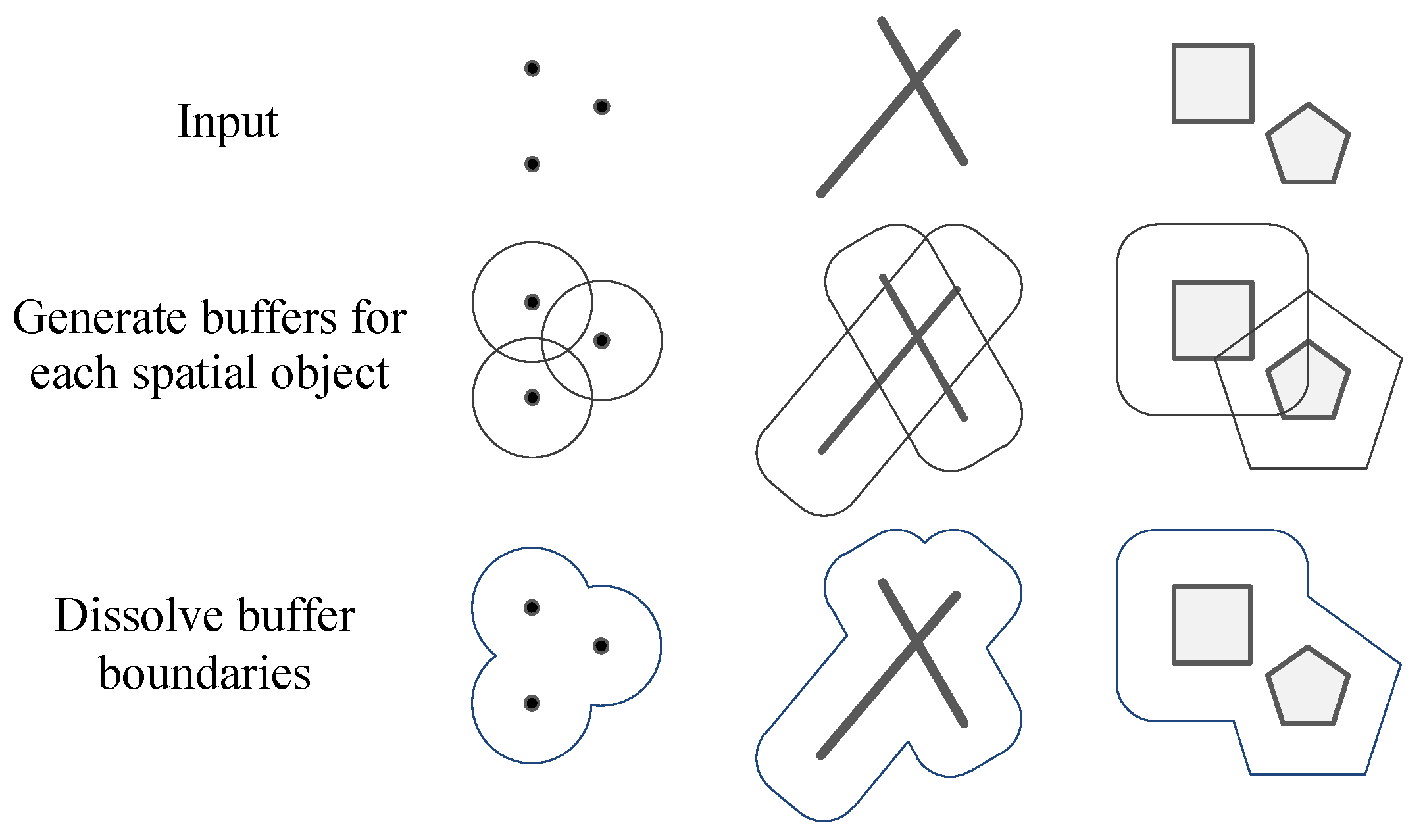Figure 2 shows the process of vector buffer generation. Compared with raster buffers, vector buffers use much less space for storage, and zooming in does not sacrifice resolution. However, in practice, circles or circular arcs in vector buffers are simplified to regular polygons or regular-polygon segments to reduce computational complexity. As shown in Figure 1b, distortion occurs in vector buffers while zooming in.

Buffer generation is computationally demanding. Furthermore, with the rapid development of surveying and mapping technology, spatial data with a larger scale are produced, which will surely increase the computational complexity of buffer generation. Previous studies have proposed many strategies to optimize the problem. Most of the optimization strategies focus on accelerating the construction of buffer zones. For vector-based methods, many approaches have been put forward to address the buffer boundary-dissolving problem [2,3,4]. Although excellent performance has been achieved, the optimized methods are implemented based on the serial approach. Therefore, the performance is limited when processing large-scale spatial data. Developments in parallel computing technologies provide a prerequisite for high-performance buffer generation, and several parallel strategies have been proposed to solve the bottlenecks [5,6,7,8].

In most existing studies, buffers of spatial objects are generated separately first, and then the buffers are merged to get the final results. Such an approach is data-oriented and straightforward. However, the computational scales expand rapidly with the volume of spatial objects; as a result, it is difficult for the traditional data-oriented methods to provide real-time buffer analysis of large-scale spatial data.

In this paper, we present a visualization-oriented parallel buffer analysis model, HiBuffer, to provide an interactive and online buffer analysis of large-scale spatial data. Different from traditional data-oriented methods, the core problem of HiBuffer is to determine whether the pixels for display are in the buffer of a spatial object or not. To the best of our knowledge, the approach is a brand new idea for buffer generation with the following advantages: (1) real-time analysis; (2) unlimited precision; (3) insensitive to data volumes. Many approaches have been proposed to achieve satisfactory performance. One feature of HiBuffer is an efficient buffer generation method, in which spatial indexes and a corresponding query strategy are incorporated. Organized into a tile-pyramid structure, the buffer results of HiBuffer are provided to users with a stepless zooming feature. Moreover, a fully optimized hybrid parallel processing architecture is proposed in HiBuffer to achieve a real-time buffer for large-scale spatial data. Using real-world datasets, we designed and conducted plenty of experiments to evaluate the performance of HiBuffer, including the real-time property, the parallel scalability, and the influence of spatial data density, buffer radius, and request rate.

The remainder of this paper proceeds as follows. Section 2 highlights the related work and literature. In Section 3, the techniques of HiBuffer are described in detail. The experimental results are presented and discussed in Section 4, with an online demonstration of HiBuffer introduced in Section 5. Conclusions are drawn in Section 6.

2. Related Work

The calculation of buffers is an essential operation of GIS. According to the computing architecture, studies on the problem can be classified into two categories: the calculation of buffers using a serial computing model and the construction of buffers in a parallel computing framework.

The first category mainly concentrates on the generation of a buffer zone for each spatial object. Dong [9] introduced a method which utilizes the rotation transform point formula and recursion approach to accelerate buffer generation. Ren [10] proposed a method that reduces the computation by removing the non-characteristic points from the original geometry based on the Douglas–Peucker algorithm. Peng [11] introduced a method based on expansion operations in mathematical morphology, in which the vector data are rasterized and expanded to generate buffers. Wang [12] introduced buffer generation methods based on a vector boundary tracing strategy. Jiechen [13] proposed a method using run-length encoding to encode raster buffers. The method reduces memory occupation while creating the buffers. Zalik [14] presented an algorithm for constructing the geometric outlines of a given set of line segments by using a sweep-line approach. Based on Zalik’s method, Sumeet Bhatia [15] presented an algorithm for constructing buffers of vector feature layers and dissolving the buffers based on a sweep-line approach and vector algebra.

With the development of computer hardware, there has been a rapid expansion in processor numbers, thus making parallel computing an increasingly important issue for processing large-scale spatial data. Parallel computing is an effective way to accelerate buffer generation.

Pang [16] proposed a method for buffer analysis based on a service-oriented distributed grid environment. The method includes a master-slave architecture, in which all the entities are assigned to slave computing nodes equally, and then the master node combines the results from all slave nodes to generate the final buffer zones. Huang [5] introduced parallel buffer algorithm which consists of a point-based partition method and a binary-union-tree-based buffer boundary-dissolving method. Fan [6] proposed a parallel buffer algorithm based on area merging to improve the performance of buffer analysis on processing large datasets. Wang [17] proposed a parallel buffer generation method based on the arc partition strategy, which achieves a better load balance performance than the point partition strategy.

In our previous work, we proposed a parallel vector buffer generation method, the Hilbert Curve Partition Buffer Method (HPBM) [8], that takes advantage of the in-memory architecture of Spark [18]. HPBM is based on the Hilbert filling curve to aggregate adjacent objects and thus to optimize the data distribution among all distributed data blocks and to reduce the cost of swapping data among different blocks during parallel processing. Experiments showed that the proposed method outperforms current popular GIS software and existing parallel buffer algorithms. However, HPBM failed to generate buffers for large-scale spatial data in real time.

In summary, all the methods mentioned above are data-oriented and straightforward, with the computational scales expanding rapidly with the volume of spatial objects. It is difficult for the traditional data-oriented methods to provide buffer analysis of large-scale spatial data in real time, though parallel acceleration technologies are adopted.

3. Methodology

In this section, the key technologies of HiBuffer are introduced. Specifically, HiBuffer is used for the buffer analysis of point and linestring objects, which are commonly used to represent points of interest (POI) and roads in maps. In HiBuffer, buffer generation is visualization-oriented; namely, the core problem of HiBuffer is to determine whether the pixels for display are in the buffer of any spatial object or not.

In HiBuffer, we utilize spatial indexes to determine whether a pixel is in the buffers of spatial objects, and accordingly, an efficient buffer generation method named Spatial-Index-Based Buffer Generation (SIBBG) is proposed. The buffers generated by SIBBG are actually raster based. To avoid the sawtooth distortion of these buffers, we propose the Tile-Pyramid-Based Stepless Zooming (TPBSZ) method. To support real-time buffer analysis of large-scale spatial data, parallel computing technologies are used to accelerate computation, and thus we designed the Hybrid-Parallel-Based Process Architecture (HPBPA).

3.1. Spatial-Index-Based Buffer Generation

Spatial indexes are used to organize spatial data. As an efficient tree data structure widely used for indexing spatial data, R-tree was proposed in 1984 [19] and has been thoroughly studied by researchers [20,21]. The spatial queries using R-tree, including the bounding-box query and nearest-neighbor search, have been fully optimized theoretically and practically. In SIBBG, we utilize R-tree to determine whether a pixel is in the buffers of spatial objects.

As shown in Figure 3, the problem in determining whether a pixel P is in the buffers, given a radius R, can be abstracted as determining whether the circle of radius R centered at P intersects with any spatial objects. An intuitive solution to the problem is as follows: (1) calculate the vector buffer $Circ$ of P with radius R; (2) use the INTERSECT operator provided by R-tree to determine whether $Circ$ intersects with any spatial objects. However, there are some disadvantages to this approach. Firstly, as shown in Figure 1b, in fact, $Circ$ is not a circle but a regular polygon; thus, it will lead to a calculation error. Secondly, as R-tree is implemented by grouping nearby objects and representing them with their minimum bounding rectangle in the next higher level of the tree, R-tree works well only for a bounding-box query, rather than queries using other polygon shapes like $Circ$.

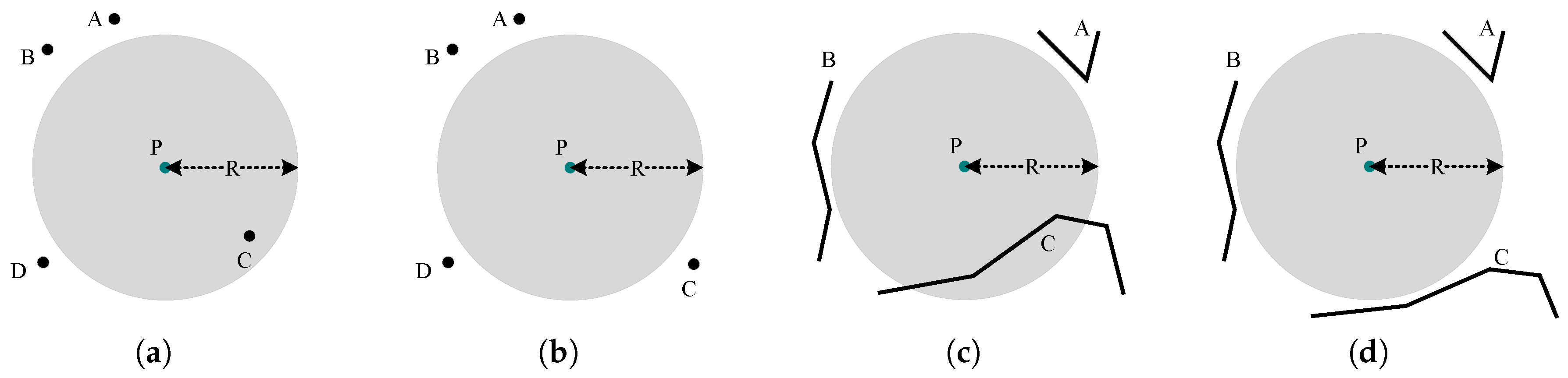
As the nearest-neighbor search has a much higher computation complexity than the bounding-box query in R-tree, we introduced inner and outer boxes (Figure 4) to optimize the spatial queries in SIBBG. The process of SIBBG is described in Algorithm 1. The inner and outer boxes are used to deal with different situations. In the situation where there are lots of spatial objects within the distance R from P, we query the spatial objects intersecting with the inner box, as a high density of spatial objects in the neighbor is very likely to intersect with the inner box; for the situation where there are few spatial objects in the neighbor of P, we use the outer box to filter out the spatial objects which are far from P. Compared with traditional methods, the performance of SIBBG is less sensitive to the data size.

Algorithm 1 Spatial-Index-Based Buffer Generation.

Input: Pixel P, radius R, and spatial index R-tree.

Output: True or False (whether P is in the buffers of spatial objects with a given radius R).

$r\leftarrow R\times \frac{\sqrt{2}}{2}$

$InnerBox\leftarrow$ box($P.x-r$, $P.y-r$, $P.x+r$, $P.y+r$)

$Tmp\leftarrow$ satisfying $Rtree$.intersect($InnerBox$)

if $Tmp$ is not $null$ then return True

else

$OuterBox\leftarrow$ box($P.x-R$, $P.y-R$, $P.x+R$, $P.y+R$)

$Tmp\leftarrow$ satisfy $Rtree$.intersect($OuterBox$) and $Rtree$.nearest(P)

if $Tmp$ is not $null$ && distance($Tmp$, P) $\le R$ then return True

return False

3.2. Tile-Pyramid-Based Stepless Zooming

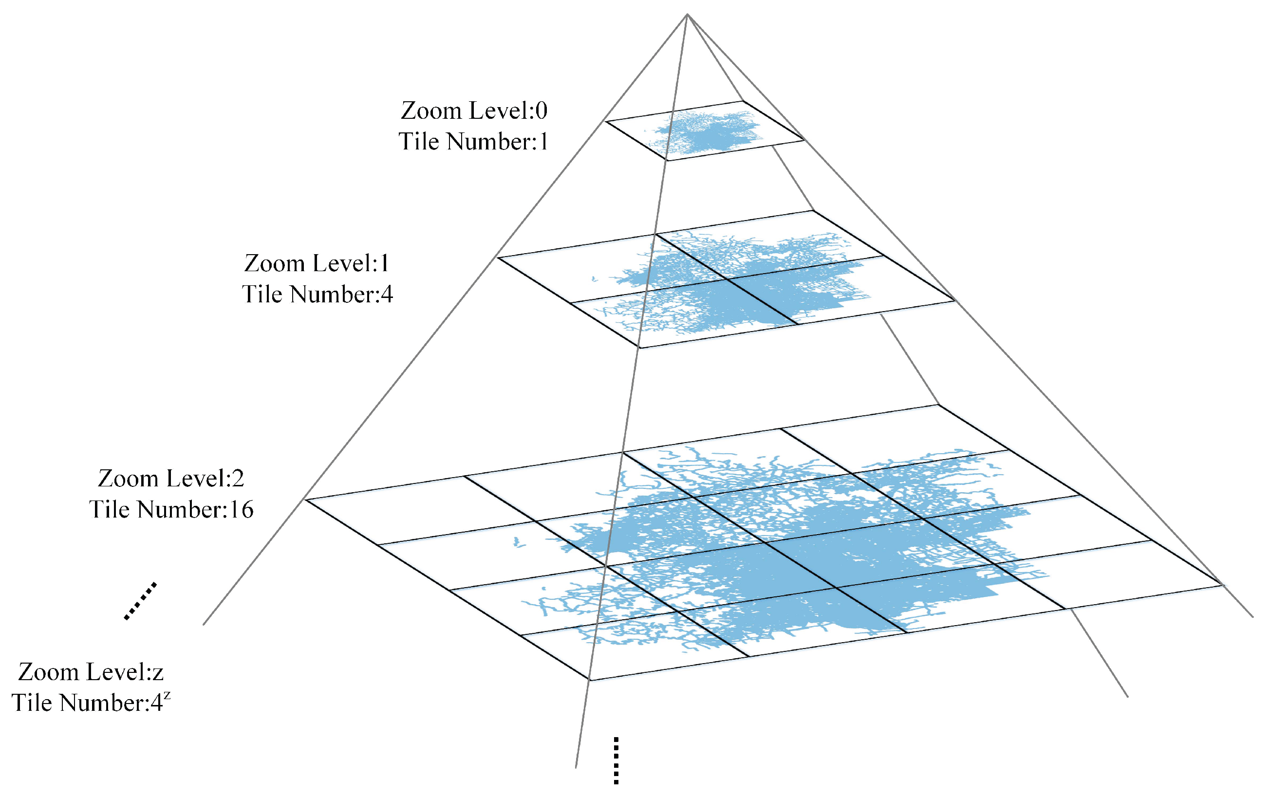
Tile-pyramid is a multi-resolution data structure model widely used for map browsing on the web. The structure of tile-pyramid is shown in Figure 5. At the lowest level of tile-pyramid (level 0), a single tile summarizes the whole map. For each higher level, there are up to $4^z$ tiles, where z is the zoom level. Each tile has the same size of $n\times n$ pixels and corresponds to the same geographic range [22]. In TPBSZ, a tile-pyramid structure is employed to organize buffer results, provided as a Web Map Tile Service (WMTS). Typically, the tile size is set to $256\times 256$ pixels, which is commonly used in tile-pyramid structures.

The advantages of TPBSZ are mainly reflected by the following two aspects:

• (Stepless zooming with unlimited precision) Tiles of different levels are selected for the screen display according to zoom levels. Zooming in on the buffer results, tiles with higher levels and higher resolutions will be used, and there is no sawtooth distortion. Besides, there is no limit on the max level; in other words, there is no highest resolution limit.
• (Stable computational complexity) The buffer results are accessed by users via a web browser, and only tiles in the screen range need to be generated. As under different zoom levels, the number of tiles in the screen range is limited and stable, the computational complexity remains stable.

3.3. Hybrid-Parallel-Based Process Architecture

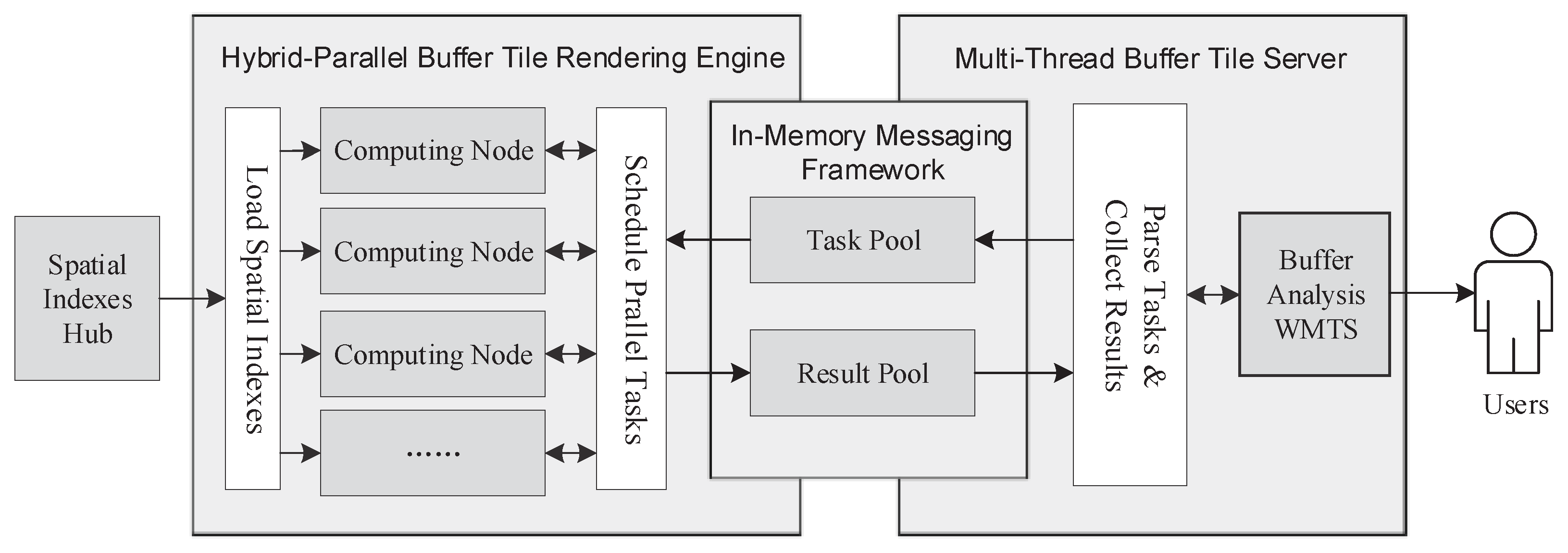
In HiBuffer, hybrid parallel computing technologies are introduced to achieve real-time buffer analysis of large-scale spatial data. The HPBPA of HiBuffer is shown in Figure 6. HPBPA mainly comprises three parts: the Hybrid-Parallel Buffer Tile Rendering Engine, Multi-Thread Buffer Tile Server, and In-Memory Messaging Framework. The Spatial Indexes Hub consists of the R-tree indexes of the spatial objects. The R-tree indexes are pre-built quickly and stored in memory-mapped files [23], which will not be totally loaded into the memory. It yields the benefits of less disk I/Os and less memory consumption, even if the indexes are very big. Task Pool stores the tasks to be executed. Analysis results are provided to users as a WMTS, which can be browsed through the Internet. The buffer tiles are created when it is requested for the first time, and the tiles are stored in the Result Pool to reduce repeated computation if the tiles are requested again.

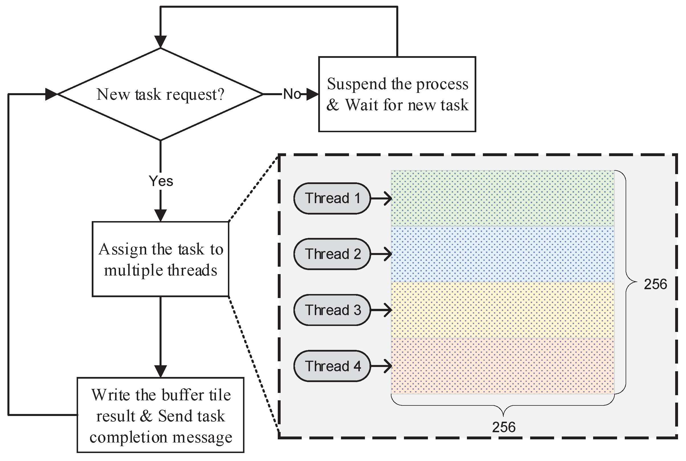
The Hybrid-Parallel Buffer Tile Rendering Engine adopts the hybrid Message Passing Interface (MPI)-Open Multiprocessing (OpenMP) parallel processing model to render buffer tiles. MPI is a multiprocess parallel processing model based on message passing. OpenMP is a multi-thread parallel processing model based on shared memory. In HiBuffer, we treat the rendering of one buffer tile as an independent task, and each task is processed with multiple OpenMP threads in one MPI process. As the task requests are generated by way of streaming, the tasks are dynamically allocated to the MPI processes. An MPI process will be suspended after the assigned task is accomplished, and new tasks will be handled on a first-in-first-served basis. An example of the buffer tile rendering process is shown in Figure 7.

The Multi-Thread Buffer Tile Server encapsulates the buffer analysis service as a WMTS. It adds tasks to the Task Pool and filters out unnecessary task requests, including (1) tiles for which the distance from Minimum Bounding Rectangle (MBR) of the spatial objects are larger than the given buffer radius; (2) tiles generated in previous tasks which are still in the Result Pool. Buffer tiles are returned to users from the Result Pool once finished. In order to improve concurrency, multi-thread technology is adopted in the tile server.

The In-Memory Messaging Framework is a messaging framework based on Redis, which is an In-Memory Key-Value database. In this messaging framework, tasks and results are transferred rapidly in memory without disk I/Os. The tasks are stored in a FIFO queue in Redis. Tasks are pushed to the queue and popped to suspended MPI processes. To avoid errors in parallel processing, the push and pop operations are performed in blocking mode. After a task is finished, the buffer tile is written to Redis, and a task completion message will be sent to the tile server using subscribe/publish functions in Redis. Tiles are set with expired times, and expired tiles are cleaned up once the max memory limit is exceeded.

4. Experimental Evaluation

In this section, we report several experiments we conducted to evaluate the performance of HiBuffer. First, the ability of HiBuffer to support real-time buffer analysis of large-scale data was tested. Then, we carried out experiments to analyze the influence of different factors on HiBuffer, including spatial data density, buffer radius, and request rate. Finally, the parallel scalability of HiBuffer was tested by running it with varying numbers of MPI processes and OpenMP threads.

4.1. Experimental Setup and Datasets

All the experiments were conducted in an SMP server, shown in

Table 1. Experimental environment.

Item	Description
CPU	32 cores*2, Intel(R)Xeon(R)[email protected] GHz
Memory	256 GB
Operating System	Centos 7.1

. The code of HiBuffer was implemented using C++ language. The experiments are based on MPICH 3.4, Boost C++ 1.64, and Geospatial Data Abstraction Library 2.1.2.

Table 2. Datasets used in the experiment.

Dataset	Abbreviation	Records	Size
OSM Beijing roads	L${}_1$	40,927	203,413 segments
OSM Taiwan roads	L${}_2$	208,067	2,336,250 segments
OSM Switzerland roads	L${}_3$	597,829	6,991,831 segments
OSM Spain roads	L${}_4$	3,132,496	42,497,196 segments
China roads	L${}_5$	21,898,508	163,171,928 segments
OSM Spain points	P${}_1$	355,105	355,105 points
China points	P${}_2$	20,258,450	20,258,450 points

shows the datasets used in the experiments. L${}_1$, L${}_2$, L${}_3$, L${}_4$, and P${}_1$ are from OpenStreetMap, which is a digital map database built through crowdsourced volunteered geographic information. The larger datasets, L${}_5$ and P${}_2$, were provided by map service providers. It is worth noting that all the datasets were collected from the real world and have a geographically unbalanced distribution property. Such datasets create challenges with respect to efficient processing.

In the experiments, a task refers to the request of a buffer tile which is in the MBR of spatial objects and also is not in the Result Pool. The rendering time of a tile refers to only the time when the tile is rendered in the Hybrid-Parallel Buffer Tile Rendering Engine, not including the waiting time while the task is in the Task Pool; the rendering time of N tiles ($N>1$) refers to the whole time cost of rendering N tiles in HiBuffer, which means from the time N tasks are generated in the Task Pool until all the tasks have been finished. The experimental settings are listed in

Table 3. Experimental settings.

Experiments	Buffer Radius (m)	Request Rate (tiles/s)	MPI Processes	OpenMP Threads
1	200	INF	32	2
2	200	INF	32	2
3	200/400/600/800/1000/100,000	INF	32	2
4	200	50/100/200/400/800/INF	32	2
5	200	INF	1/2/4/8/16/32/64	1/2/4

. The benchmark buffer radius was set to 200 m, which has practical meaning for the datasets with a wide spatial range. The benchmark request rate was set to infinity, which means that all the task requests are dispatched simultaneously. As there are 32 cores/64 threads in the server processors, the benchmark parallel processing was set to run with 32 MPI processes and 2 OpenMP threads in each process.

4.2. Experiment 1: Support Real-Time Buffer Analysis of Large-Scale Data with HiBuffer

In order to highlight the superiority of HiBuffer,

Table 4. Performance of traditional data-oriented methods [8] and HiBuffer.

Algorithm	${\mathbf{L}}_1$		${\mathbf{L}}_2$		${\mathbf{L}}_3$
	Latency(s)	Speedup	Latency(s)	Speedup	Latency(s)	Speedup
HPBM	9.0	/	38.8	/	332.3	/
Method${}_1$ ${}^{\mathrm{a}}$	15.4	1.7	128.2	3.3	936.9	2.8
Method${}_2$ ${}^{\mathrm{b}}$	12.3	1.4	75.5	1.9	661.9	2.0
Method${}_3$ ${}^{\mathrm{c}}$	17.2	1.9	220.8	5.7	2813.4	8.5
PostGIS	34.9	3.9	295.8	7.6	2380.2	7.2
QGIS	129	14.3	2788	71.9	>7200	>7200
ArcGIS	139	15.4	2365	61.0	>7200	>7200
HiBuffer	<1	/	<1	/	<1	/

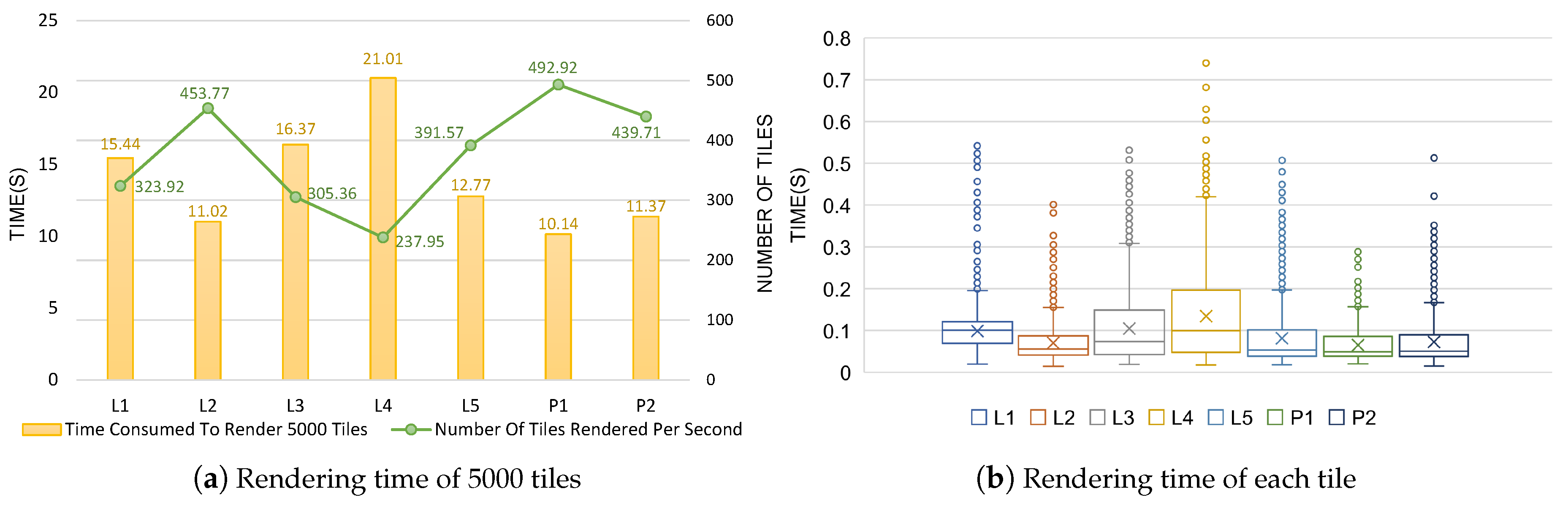
^a is based on three optimization methods: split-and-conquer buffer zone generation, vertices-based task decomposition, and tree-like merger [6]. ^b adopts strategies such as vertices-based task decomposition and tree-like merger [5]. ^c uses the equivalent-arc partition strategy [17].

shows a comparison of HiBuffer with HPBM, three optimized parallel methods, and the popular GIS software programs PostGIS, QGIS, and ArcGIS. HiBuffer was deployed and tested in the same hardware environment. We then carried out experiments on the tile rendering time to further evaluate the real-time characteristic of HiBuffer. For each dataset, we generated 5000 tasks through a test program, which requested different buffer tiles at different zoom levels randomly. We analyzed the tile rendering logs, and the experimental results are shown in Figure 8.

As shown in Table 4, HPBM outperformed the other traditional data-oriented methods. However, HPBM failed to generate buffers for large spatial data in real time. Even for a small dataset, such as L${}_1$, it took 9 s for HPBM to generate the buffer result. As data volumes grew, the computing time using traditional methods increased significantly. Typically, from L${}_2$ to L${}_3$, the data size rose from 2,336,250 segments to 6,991,831 segments (around 3 times), while the computing time using HPBM increased from 38.8 s to 332.3 s (around 8.6 times). The reason for the differing increase rates is that different data distributions led to different buffer zone dissolving complexities. As a result, it is almost impossible to generate buffers for massive spatial data in real time using traditional data-oriented methods. Using HiBuffer, we can get the buffer results for the datasets (L${}_1$, L${}_2$, L${}_3$) in less than 1 s.

Figure 8a shows the time consumed to render 5000 buffer tiles for each dataset. From L${}_1$ to L${}_5$ or P${}_1$ to P${}_2$, the data size increases sequentially; however, there is no significant uptrend in the rendering time of 5000 buffer tiles. Surprisingly, L${}_5$, the largest dataset with more than 20 million linestring objects, produces better performance than the datasets with much smaller scales (L${}_1$, L${}_3$ and L${}_4$). The experimental results show that HiBuffer is insensitive to data volumes. In Figure 8a, the number of tiles rendered per second is calculated. L${}_4$ produces the poorest performance with 237.95 tiles per second. As the number of tiles in a screen is generally no more than 50, it is possible to perform real-time buffer analysis with HiBuffer for all the datasets. As shown in Figure 8b, the rendering time distributions of each tile on different datasets are visualized with boxplots (‘○’ represents outliers and ‘×’ represents average rendering time). For all the datasets, L${}_4$ produces the poorest performance though; most of the requested buffer tiles of L${}_4$ are rendered in 0.45 s, with the longest rendering time not exceeding 0.75 s. It is assumed that a browser requests 50 buffer tiles of L${}_4$ at once. Considering that there are 32 MPI processes, the 50 tasks will be processed in two rounds, with 14 ($={32}_{\mathrm{processes}}\times 2-{50}_{\mathrm{tasks}}$) MPI processes suspended in the second round: namely, it will be most likely completed in less than 0.9 s ($=0.45\mathrm{s}\times 2$). In conclusion, HiBuffer is able to provide interactive and online buffer analysis of large-scale spatial data, which is difficult for traditional data-oriented methods.

4.3. Experiment 2: Impact of Spatial Data Density in HiBuffer

In this experiment, we focused on testing the impact of spatial data density on HiBuffer. Spatial data density refers to the number of spatial elements per unit area. We used the number of segments or points in a tile to signify spatial data density. To express spatial data density exactly, the tile level should be neither too low nor too high. Typically, we chose tiles of level 13, which have proper spatial spans (about 4.9 × 4.9 km) for all the datasets. For each dataset, we generated 5000 different requests of buffer tiles of level 13 and studied the relationship between tile rendering time and the number of elements in the tiles. The results are shown in Figure 9.

Figure 9a–g illustrate the changes in tile rendering time, along with the increase in element numbers in a tile for each dataset. A point (‘○’) in the figures represents a sample with a record of rendering time of a tile and number of elements in the tile. The trend lines, generated based on the lowess regression, indicate the trends of the changes. As shown by the trend line of each dataset, the rendering time of a tile has an uptrend, along with the increase in element numbers in a tile, which means the performance decreases with the increase in spatial data density in HiBuffer. This is because higher spatial data density leads to higher computational complexity in the SIBBG process. However, the performance degradation in HiBuffer is not serious (take L${}_4$, for example: when the number of segments in a tile increases to about 28,000, the rendering time of the tile is still less than 0.5 s). The percentage lines illustrate the distributions of 5000 tiles under different spatial data densities, which demonstrate the geographically unbalanced distribution property of the datasets. Figure 9h compares the impact of spatial data density on the different datasets. The average number of elements in the tiles indicates the spatial data density of a dataset, while the average rendering time of each tile indicates the buffer generation performance. As illustrated in the figure, the spatial data density and the performance roughly have the same trend. This shows that datasets with higher spatial data density yield a weaker performance in HiBuffer, which explains the experimental phenomenon that HiBuffer is insensitive to data volumes. L${}_5$ has the largest data volume though, and the lower the spatial data density, the better the performance produced compared with datasets with much smaller scales. Also, the reason that L${}_1$, the small dataset, results in a weaker performance is that the spatial data density is high. The average rendering time of a tile which intersects with no elements was also calculated and is shown in the figure. For different datasets, the average rendering time of a no-element tile always remains at about 0.05 s. This demonstrates that the rendering time of a no-element tile is not related to the spatial data densities or the data volumes of the datasets.

4.4. Experiment 3: Impact of Buffer Radius on HiBuffer

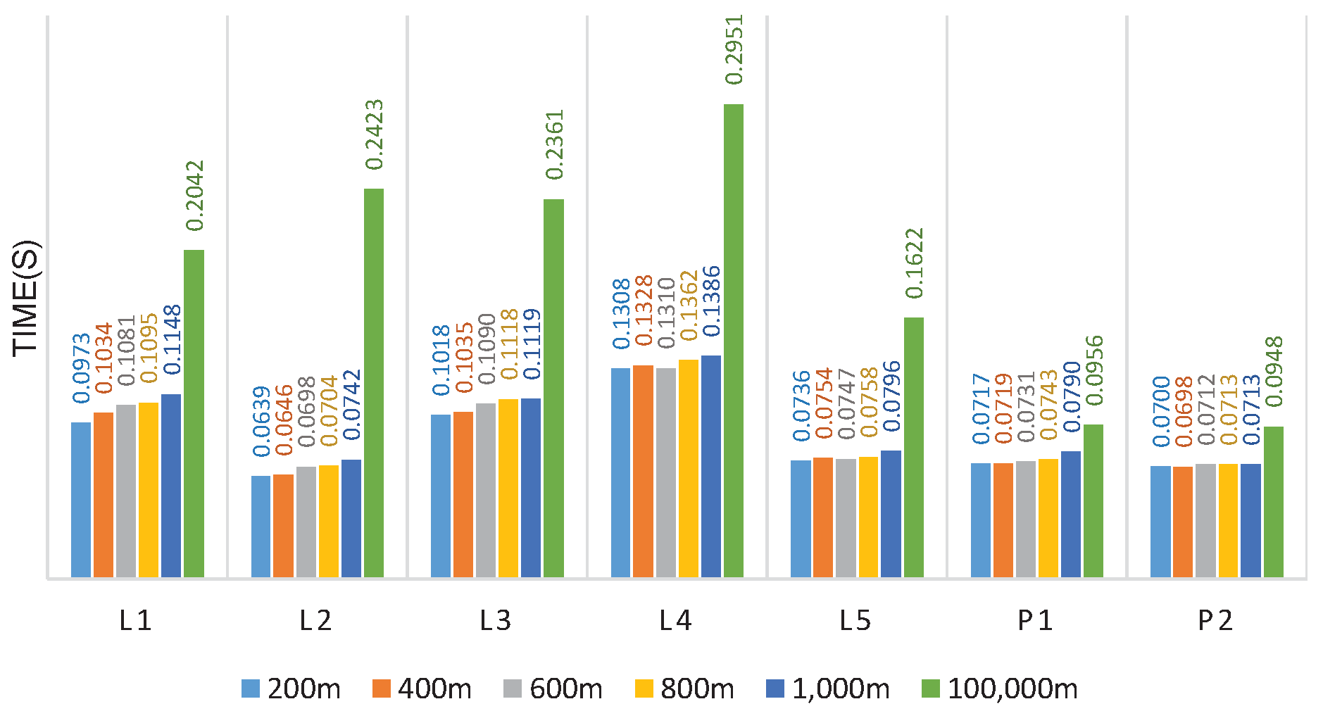
In experiment 3, the impact of the buffer radius on HiBuffer was studied. The buffer radius was set to 200, 400, 600, 800, 1000, and 100,000 m, respectively. For each radius, we generated 5000 buffer tile tasks of different zoom levels for each dataset. We calculated the average rendering time of each tile; the experimental results are shown in Figure 10.

As the buffer radius increases, more pixels in the tiles belong to the buffers of spatial objects, and more computation is required to generate the buffer tiles. This is corroborated by the experimental results: the average rendering time of each tile shows an uptrend with the increase in buffer radius for all the datasets. To estimate the lower-bound performance of HiBuffer, the buffer radius was set to a very large value, 100,000 m, which is 500 times the benchmark buffer radius. The results show that when the buffer radius is 100,000 m, the performance degradation of HiBuffer is not serious. L${}_4$ produces the poorest performance though; the average rendering time of each tile for L${}_4$ is 0.2951 s, which can still support real-time buffer analysis.

4.5. Experiment 4: Impact of Request Rate on HiBuffer

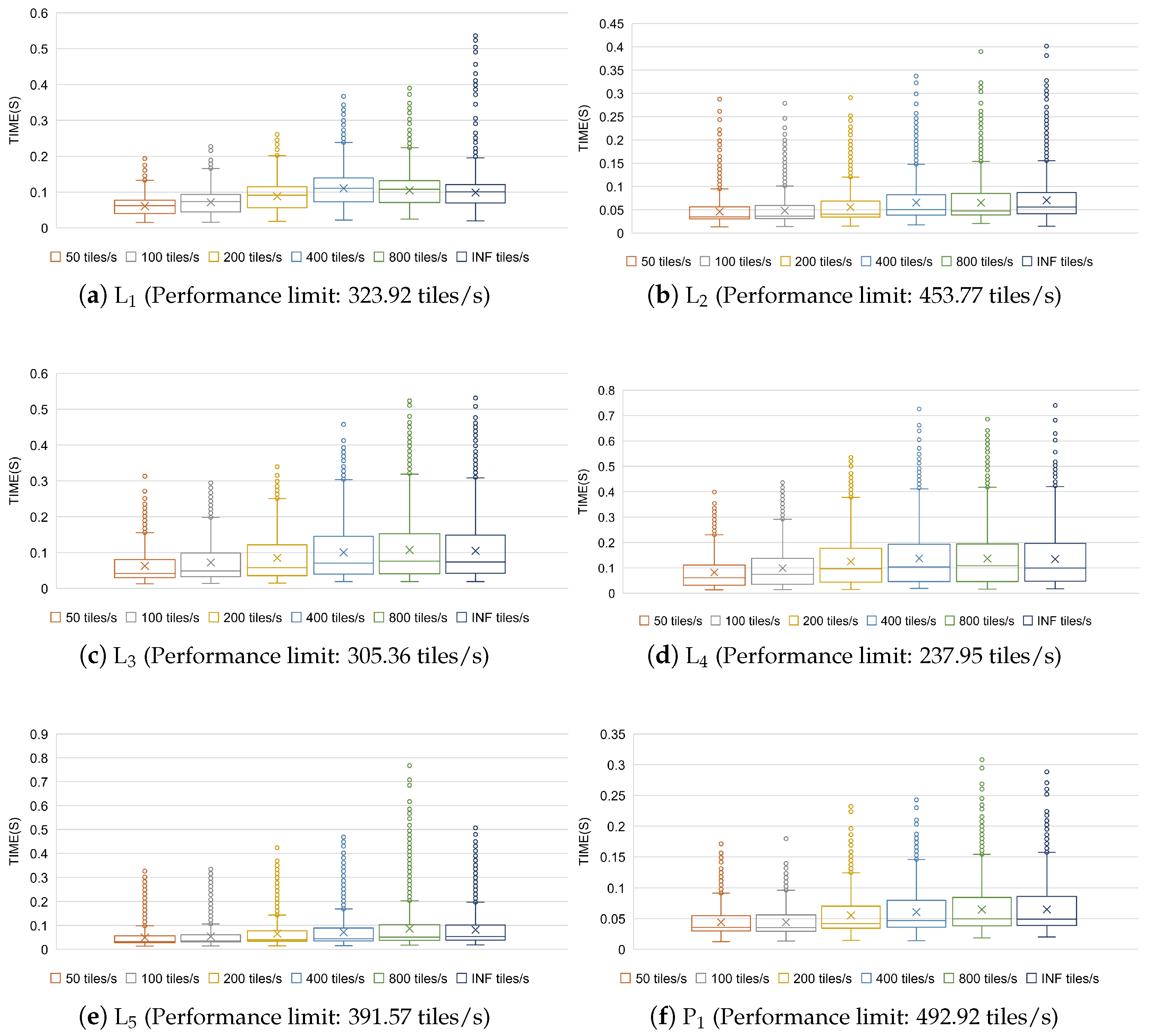
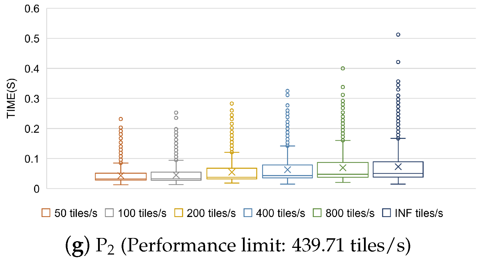
With the exception of experiment 4, the request rate was set to infinity in all other experiments. This means that all the task requests were dispatched simultaneously, and HiBuffer kept running at full load until all tasks were finished. In practical applications, however, the task requests are generated by way of streaming at much lower request rates. In this experiment, the request rate was set to 50, 100, 200, 400, 800, and INF tiles per second, respectively. For each rate, we generated 5000 buffer tile tasks for each dataset.

The rendering time distributions of each tile with different request rates are illustrated in Figure 11. For each dataset, we used the number of tiles rendered per second at the request rate of INF tiles/s (Figure 8a) as the performance limit in HiBuffer. The performance of HiBuffer for all the datasets is affected by the request rate with roughly the same trend. When the request rate is less than the performance limit, the rendering time of a tile increases obviously with the increase in request rates. This results from the intensifying competition for resources between processes in HiBuffer. In contrast, when the request rate exceeds the performance limit, the rendering time of a tile does not change significantly. This is because HiBuffer is running at full load, and the increase in request rates does not cause an obvious effect on the tile rendering performance. However, due to the increase in waiting time while tasks are in the Task Pool, the performance of HiBuffer decreases rapidly with the increase in request rate when the request rate exceeds the performance limit. In all the experiments, other than experiment 4, the request rate was set to infinity, which indicates that compared with the experimental results, a higher performance can be achieved in practical applications as a result of the lower request rates.

4.6. Experiment 5: Parallel Scalability of HiBuffer

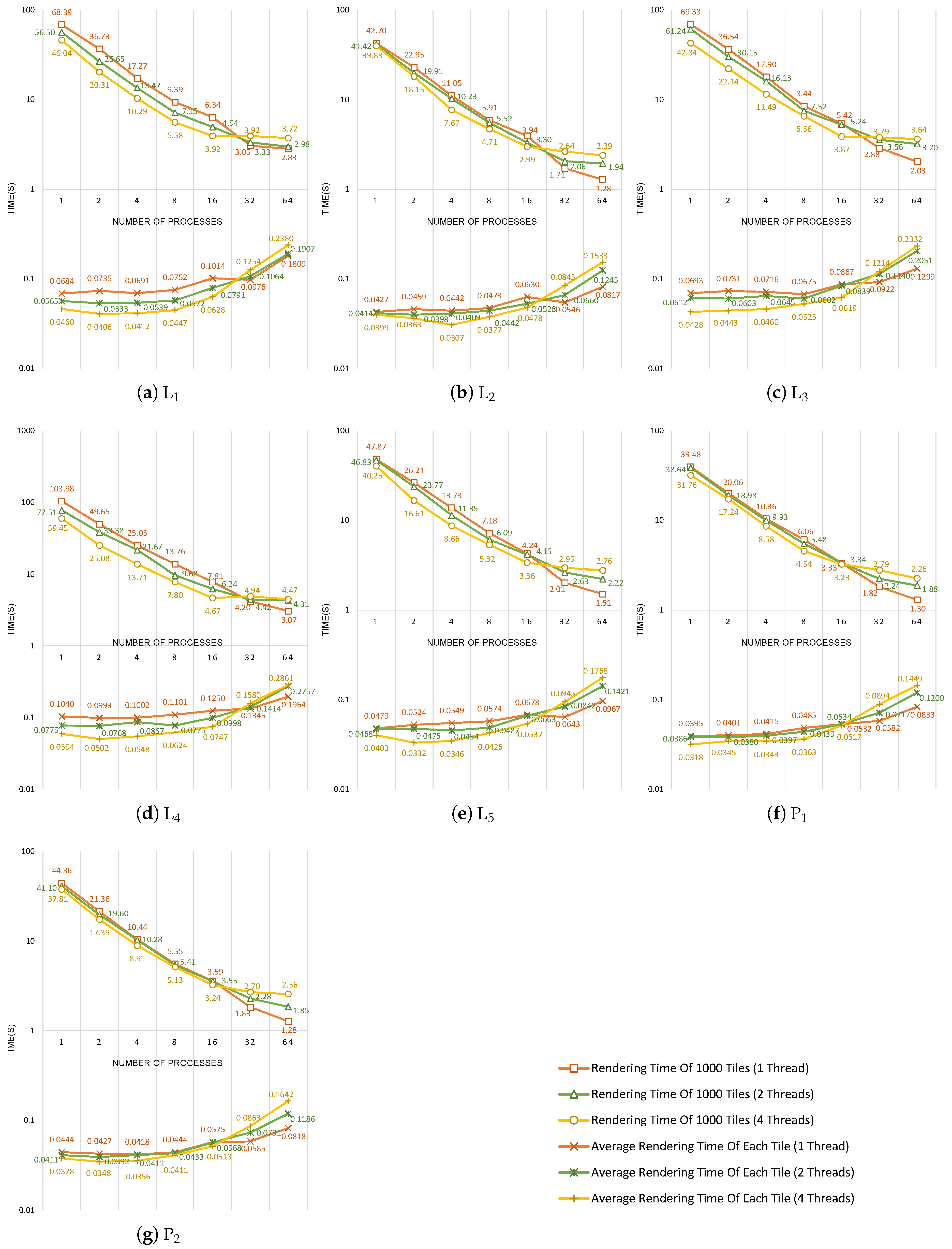
To evaluate the parallel scalability, HiBuffer was respectively tested to run on 1, 2, 4, 8, 16, 32, and 64 MPI processes with 1, 2, and 4 OpenMP threads in each process. For each pair of MPI processes and OpenMP threads, we generated 1000 buffer tile requests of different zoom levels for each dataset. The experimental results are plotted in Figure 12.

First, we analyzed the rendering time of 1000 tiles. The results show that with the increase in process numbers, HiBuffer achieves a high performance of parallel acceleration, which is approximate to linearity when the process number is below 16. However, the performance of parallel acceleration decreases as the process number is increased past 16, especially while running with 4 OpenMP threads in each process. This is because the increase in process numbers aggravates resource competition, which is even worse while running with multi-thread. For example, in Figure 12d, the rendering time of 1000 tiles with 4 threads increases even as the process numbers increase from 16 to 32. Then, we compared and analyzed the average rendering time of each tile line with different OpenMP threads. As shown in the figures, multi-thread parallel processing can effectively reduce the rendering time of a tile when resource competition is not intense. Surprisingly, multi-thread parallel processing even causes performance degradation when the process number is over 16 as a result of the resource competition.

Based on the experimental results and the analysis, we can draw some conclusions on the deployments of HiBuffer in the given hardware environment: (1) in the condition of high load, 64 processes × 1 thread is suggested, because it takes the least time to generate 1000 tiles for all the datasets; (2) in the condition of low load, 16 processes × 4 threads is suggested, as this setting has a high rendering speed of each tile and can reduce the response time of buffer tile requests while the numbers of requests are low.

5. Online Demo of HiBuffer

An online demonstration of HiBuffer is provided on the Web (http://www.higis.org.cn:8080/hibuffer). The OSM Spain roads and points (L${}_4$ and P${}_1$) were used as test data. The demonstration was deployed on a server with four cores/eight threads (see

Table 5. Environment of the online demo.

Item	Description
CPU	4 cores*2, Intel(R)Xeon(R)[email protected] GHz
Memory	32 GB
Operating System	Centos 7

) and set to run with four MPI processes and eight OpenMP threads. Compared with the experimental environment (see Table 1), there are much fewer CPU cores and much less memory space in the hardware environment of the demonstration, which will surely result in a weaker buffer analysis performance. Even so, as illustrated in the demonstration, it is still possible to provide an interactive buffer analysis even for L${}_4$, the dataset which produces the poorest performance in HiBuffer. Figure 13 shows the analysis results of the online demo.

6. Conclusions and Future Work

This paper presents a visualization-oriented parallel model, HiBuffer, for real-time buffer analysis of large-scale spatial data. In HiBuffer, we propose an efficient buffer generation method named SIBBG. R-tree indexes are utilized in SIBBG to improve buffer generation speed. The performance of SIBBG is not sensitive to the data size. We used the tile-pyramid to organize buffer results and thus propose the TPBSZ. TPBSZ produces satisfactory visualization effects of stepless zooming with unlimited precision and stable computational complexity. Parallel computing technologies are used to accelerate analysis, and we propose the HPBPA. In HPBPA, we designed the fully optimized Hybrid-Parallel Buffer Tile Rendering Engine, Multi-Thread Buffer Tile Server, and In-Memory Messaging Framework.

Our experimental results show that HiBuffer has significant advantages compared with data-oriented methods. Experiment 1 demonstrates the ability of HiBuffer to provide interactive and online buffer analysis of large-scale spatial data. Experiment 2 shows that the performance decreases with the increase in spatial data density in HiBuffer; however, the performance degradation is not serious. In experiment 3, we analyzed the impact of buffer radius on HiBuffer. It shows that the performance decreases slightly with the increase in buffer radius in HiBuffer, and it is still possible to support real-time buffer analysis when the buffer radius is set to 100,000 m, which is a very large value. Then, experiment 4 analyzes the impact of the request rate on HiBuffer. The result indicates that compared with the experimental results, a higher performance can be achieved in practical applications, as the request rate was set to infinity in all the experiments other than experiment 4. In experiment 5, we tested the parallel scalability of HiBuffer. The results show that HiBuffer achieves a high performance of parallel acceleration when resource competition is not intense. Moreover, an online demonstration of HiBuffer is provided on the Web.

HiBuffer does have limitations, and some directions for future research are worth noting:

• (Better computation reduction strategies) In HiBuffer, all buffer tile levels contain the same information but with different resolutions, which indicates that we can use tiles at lower levels to reduce the computation of rendering high-level tiles.
• (Buffer analysis of polygon objects) The buffer generation of point and linestring objects is well-studied in this paper, and future work will focus on applying HiBuffer to buffer analysis of polygon objects.
• (Spatial data at a global scale) In this study, the performance of HiBuffer was tested on datasets at country scales. In the future, we will apply HiBuffer to buffer analysis of global-scale datasets (e.g., the spatial data of the whole world from OpenStreetMap). To support spatial data at a global scale, more optimizations may be needed. For example, to avoid loading the spatial indexes of the whole dataset while generating a buffer tile of a small region, we can divide the spatial data into several parts and build distributed spatial indexes for each part respectively.
• (Support overlay analysis) Overlay analysis is a time-consuming geometric algorithm which combines the spatial data of two input map layers. The operations of overlay analysis include spatial intersection, difference, and union. In our future work, we will extend HiBuffer to solve overlay analysis problems.