Intact Planar Abstraction of Buildings via Global Normal Refinement from Noisy Oblique Photogrammetric Point Clouds

Abstract

Oblique photogrammetric point clouds are currently one of the major data sources for the three-dimensional level-of-detail reconstruction of buildings. However, they are severely noise-laden and pose serious problems for the effective and automatic surface extraction of buildings. In addition, conventional methods generally use normal vectors estimated in a local neighborhood, which are liable to be affected by noise, leading to inferior results in successive building reconstruction. In this paper, we propose an intact planar abstraction method for buildings, which explicitly handles noise by integrating information in a larger context through global optimization. The information propagates hierarchically from a local to global scale through the following steps: first, based on voxel cloud connectivity segmentation, single points are clustered into supervoxels that are enforced to not cross the surface boundary; second, each supervoxel is expanded to nearby supervoxels through the maximal support region, which strictly enforces planarity; third, the relationships established by the maximal support regions are injected into a global optimization, which reorients the local normal vectors to be more consistent in a larger context; finally, the intact planar surfaces are obtained by region growing using robust normal and point connectivity in the established spatial relations. Experiments on the photogrammetric point clouds obtained from oblique images showed that the proposed method is effective in reducing the influence of noise and retrieving almost all of the major planar structures of the examined buildings.

1. Introduction

The demand for the automatic three-dimensional modelling of large-scale urban environments, especially buildings, has triggered increasing research attention in recent years, for interactive mapping applications, urban planning and analysis and computational engineering [1]. Under this demand, the penta-view aerial oblique camera has acquired new popularity and soon provided the standard datasets for building reconstruction [2]. Various oblique camera systems have been developed, and massive airborne datasets have been collected. With advances in Structure From Motion (SFM) [3,4] and Multiview Stereo (MVS) [5], aerial oblique images can now be processed automatically to produce tiled dense photogrammetric point clouds at the city scale.

The use of oblique photogrammetry for three-dimensional modelling seems promising, due to the capability to obtain occlusion-free outputs from multi-view data. Unfortunately, the obtained photogrammetric point clouds are also severely noise laden [6]. In addition, unlike common outliers that could be removed during preprocessing, noise generally reflects in small fluctuations of point clouds, which may lead to problems during plane segmentation but should be considered as inliers. Therefore, the aim of this paper is to abstract the buildings by planar segments with explicit handling of the conspicuous noise level, which is a fundamental step for further level-of-detail (LOD) reconstruction. In the following sections, we first provide a brief review on surface normal estimation and different approaches for planar segment extraction; and then discuss the aims and contributions of this paper.

1.1. Related Works

Normal Estimation: The normal vectors of point clouds are fundamental geometric shape properties (i.e., representation of the geometry around a specific point) for planar segmentation and many other applications [7] and are still under active study [8,9]. There are two core steps for satisfactory normal estimation: (1) determining the selected region around each point and (2) determining the geometric kernel to fit the tangent space for the above region as shown in Figure 1. For the first issue, the most intuitive and widely adopted region is the k-neighborhood (or r-ball), based on the k-dimensional tree (kd-tree) [10]. Local region selection and covariance estimation methods may be improved by considering density anisotropy using different weightings [11] and robust statistical information [12], respectively. For the second issue, the standard approach to normal estimation is based on principal component analysis (PCA) [13], for which the geometrical interpretation is to fit a thin ellipsoid, and the direction for the minor axis is the normal vector [14]. Jet fitting [15] is another popular method that uses a quadratic surface as the geometric kernel. Other geometric kernels, including spheres and splines, can also be adapted to the smooth surface for normal estimation and the determination of other geometrical properties [16]. Recently, research has even demonstrated that the geometric kernel can be learned from exemplar datasets using deep neural networks [16]. Although the above methods with sophisticated geometrical kernels are suitable for complex shapes, urban environments (especially buildings) have planes as the primary structure, and the problem caused by noise in a local region is more serious, which requires information in a larger context to alleviate its influences, as shown in Figure 1.

Model fitting: Model fitting-based planar extraction methods can be categorized by the approaches used to determine the model, including the random sample consensus (RANSAC) [17,18] and Hough transform (HT) [19]. The HT has been used to detect various types of geometries, including planes [20] and L-shape structures [21] in point clouds. However, the time and memory required to perform a HT on a large data set are prohibitively high [22], which impedes its usage in a large scale urban environment. Although RANSAC-based methods are more robust and better at handling outliers, RANSAC generates a planar surface with a maximal number of points for every iteration, with many spurious planes that may be generated [23]. To prevent the detection of these spurious planes, follow-up works have extended RANSAC by considering local surface normal vectors [24] or combining it with a regional growing method [18]. However, as described above, the local surface property is sensitive to noise [25], which limits its usage for photogrammetric point clouds from oblique images.

Region growing: Region growing-based [26] planar extraction methods generally consist of three major factors: (1) the selection of the starting seed primitives; (2) the criteria to extend the seed region; and (3) the criteria to terminate growing. First, the choice of seed is not limited to points, but can also be triangles in a surface mesh [27] or initial planar primitives [28]. The most intuitive method to place a seed is random selection; however, if the seed primitive is located in areas with high noise, the growth regions may deviate from the expected regions. To overcome this problem, points with good planarity should be chosen for the seed points [29]. Second, for the growing criteria, the similarity of normal vectors and the distance between neighbor points and the current region are widely adopted [30,31,32]. Alternatively, neighboring patches can be applied to growing regions [33] based on minimizing the deformable energy. Third, as the region grows larger, the fitting error also monotonically increases, and the termination criteria are determined by the largest error. In an empirical evaluation, the region growing-based method has a higher recall rate on the retrieved primitive than the model fitting-based method [34], which is much slower. In addition, because only the local information in a small neighborhood context is used for growing in each iteration, the global context is ignored; therefore, the regional growing methods are intrinsically sensitive to noise and probably lead to the problem of crossing the object boundary.

Supervoxel clustering: Similar to the well-studied superpixel clustering, the clustering of points into supervoxels can also be used as an intermediate representation for further application and still remain in the developmental stage [35]. The most popular artificial method for supervoxel clustering is the Voxel Cloud Connectivity Segmentation (VCCS) [36]. VCCS first generates an adjacency graph using octree, and divides the space into a voxelized grid with a seed resolution and voxel resolution. Then, VCCS supervoxels are clustered by 39 dimensional local geometric features. VCCS supervoxels are reported to be highly efficient, and the results on RGB-D test data ensure no crossing over object boundaries. For further applications, such as object detection [37], classification [38] and segmentation [39], there are three advantages for point clouds being partitioned into supervoxels as basic entities in comparison to a single point. First, supervoxels provide more discernible structural features; second, the adjacency relationships are clearer; third, the computational complexity is significantly reduced, especially for large-scale urban scenes. Because of the advantage of reducing computational complexity and preserving boundaries, in this paper, the supervoxel is also adopted in the first stage and augmented with contextual information to overcome the noise problem.

1.2. Contributions

By aiming at overcoming the problem caused by noise and deformations in photogrammetric point clouds, the major contribution of this paper is: a global optimization technique for normal estimation, which gradually propagates the structural information from a single point gradually to a significantly larger context; region growing to extract planar segments is, therefore, also aware of the global structure. More specifically, this method proceeds in a hierarchical fashion: (1) points are merged into supervoxels, which are over-segmented representations of the point clouds and, more specifically, a planarity constraint is proposed to enforce the preservation of object boundaries; (2) the supervoxels are then expanded to collect support regions for normal estimation, which is denoted as the maximal support region; (3) global optimization is used to obtain relatively consistent normal vectors from contextual information implied by the maximum support region; and (4) using the revised normal and contextual information, region growing is conducted based on the spatial relations and similarities of the features. Based on the above workflow, the proposed method is more resilient to the influences of noise and deformations of photogrammetric point clouds and generates more intact planar segmentation.

The remainder of this paper is structured as follows. In Section 2, global normal refinement and the planar surface extraction of buildings are described. Experiments on oblique photogrammetric point clouds and the results are demonstrated in Section 3. The conclusions are provided in Section 4.

2. Methods

Planar structures are common in urban areas, and coplanar points are assumed to share the same normal vector. However, for noisy photogrammetric point clouds, planar surfaces may not appear to be flat, leading to inaccurate segmentation. In this paper, a robust approach is presented to segment photogrammetric point clouds based on global normal estimation to overcome noise. As shown in Figure 2, the point clouds are preprocessed using supervoxel clustering, and a planarity constraint is proposed to enforce the preservation of object boundaries, and effectively reduce the number of inputs (from millions to thousands) without the loss of sharp features (Section 2.1). Then each supervoxel cluster grows to the size of the maximum planar support regions; this process is similar to regional growing, except that a strict termination condition is incorporated to further preserve the boundary (Section 2.2). Neighborhood connectivity is generated from all of the support regions, which is used as the observation during global optimization to reorient the initial normal vectors into consistent directions (Section 2.3). Finally, planar surfaces are segmented by region-growing, which combines the robust normal vectors and spatial relations between among those that are established in the previous steps (Section 2.4).

2.1. Boundary-Preserved Supervoxel Clustering

The objective of supervoxel clustering is to (over-)segment the point cloud into small regions that are assumed to have uniform sizes, convex shapes, and connectivity information in a local region. Formally, given point clouds P = {p₁, p₂, …, p_n}, this step splits P into different clusters, C = {c₁, c₂, …, c_m}, where each cluster c_i contains a non-overlapping subset of P. Our proposed implementation is motivated by the VCCS [36], which is publicly available in the PCL (point cloud library) [40]. However, as the original method is designed in a sequential iterative way and the clustering is, in fact, the bottleneck of the whole pipeline, we propose a parallel extension of the original supervoxel clustering method and furthermore, a boundary constraint is enforced to preserve sharp features.

Supervoxel clustering begins with building an octree spatial index of point clouds, which explicitly generates a 26-adjacent connectivity graph in neighborhood of 3 × 3 × 3 cubes [41]. Other than general purposing segmentation methods, which may produce elongated or non-convex regions, the objective of supervoxel clustering is to (over-)segment the point cloud into small regions that are assumed to have uniform sizes, convex shapes, and connectivity information in a local region. The seeds for the initial supervoxels are uniformly selected in the octree. The core step in clustering the supervoxels is to expand or exchange the leaves of the octree with their direct adjacent neighbors in each iteration. This step iterates several times and is determined by the search radius. The criteria for expansion are measured by the feature distances from the leaf points. Instead of using the original 39-dimensional features, we have found that a simpler 9-dimensional feature containing three categories of features is sufficient for each point p_i in urban environments:

$$f_i={\left[x,y,z,L,a,b,n_x,n_y,n_z\right]}^T$$

(1)

where [x, y, z]^T represents the spatial position, [L, a, b]^T represents the color in CIE space, and [n_x, n_y, n_z]^T represents the noisy normal vector estimated with the orientation determined from the viewpoint of the aerial oblique images of the SFM-MVS pipeline. Normal vectors are used instead of the FPFH (fast point feature histograms) feature [42], because they are more intuitive and efficient in constraining planar structures. The feature distance is also normalized and weighted from the three categories, as in the original method of Papon et al. [36]. For original implementation, the expansion of all of the leaf points is implemented sequentially and becomes the bottleneck for the whole pipeline. In this paper, this step is parallelized by caching the provisional testing results and updating all supervoxels after a whole epoch of expansion tests. In practice, we found no significant difference between the two strategies, but there was almost a linear speedup with respect to the number of parallel threads.

Because the expansion test uses noisy initial normal vectors, we have found that a certain amount of supervoxels may still cross the object boundary. To remedy this problem, a refinement step follows, which swaps the boundary-crossing points between two adjacent supervoxels. Based on the planar assumption, the spectral features of points are used to measure the planarity of each supervoxel, which can be calculated by the eigenvalues of the singular value decomposition (SVD) of the covariance matrix of the points [43]. We let the eigenvalues and eigenvectors be σ₁ < σ₂ < σ₃ and η₁, η₂, η₃, respectively. The following constraint is adopted:

$$\{\begin{array}{l}{\sigma }_2/{\sigma }_1>{\tau }_1\\ {\sigma }_3/{\sigma }_2<{\tau }_2\end{array}$$

(2)

where the top row enforces the planarity of the point clouds and the bottom row prevents the occurrence of elongated shapes, which we found common in the intersections of the two faces. The thresholds of 45 and 15 were selected as common values [38,44] for τ₁ and τ₂, respectively.

For the boundary-crossing supervoxels, they are again isolated into points and should be re-assigned to adjacent supervoxels. Thus, for each isolated point, we add it to the adjacent supervoxels separately and recalculate the covariance matrixes and planarity. Each point is sequentially tested against adjacent supervoxels and the simple winner-take-all strategy is adopted to assign the point. After refinement of the boundary-crossing supervoxels, the centroid of each supervoxel is updated, and a plane is fitted to the points; the normal vector of the plane can be regarded as the normal vector of the supervoxel. The adjacencies of the supervoxels are then estimated through a K-nearest neighbor (KNN) search of the centroids c_i, which improves the successive growth of the maximum planar support region, as described below.

2.2. Hierarchical Generation of the Maximum Planar Support Region

Although planarity can be internally preserved in each supervoxel, sufficient structural information cannot be retrieved from a single supervoxel. Therefore, in this step, each supervoxel grows to the adjacent supervoxels to enclose larger contextual information: the maximum planar support region. Specifically, we obtain a support region by enclosing adjacent supervoxels for each c_i, where S_i = {c_i, c_j ∈ C|j = 1, 2, …, n, j ≠ i}, and S is assumed to be planar.

The support region for each supervoxel is generated in a region-growing manner. As described above, KNN is used for the adjacency search, which is conducted using a coarse-to-fine strategy by changing the value of k. (1) a larger neighbor set, N_i ∈ C, is created around the supervoxel c_i (k = 16); (2) the success of the expansion is tested, as described later; (3) if the expansion fails, k is decreased by a factor of two; and (4) steps (2) and (3) are repeated until no supervoxel is inserted, as shown in Figure 3c. In practice, the expansion may fail if the supervoxel is located around a sharp feature, because the neighbor set around the supervoxel may cross the sharp feature. Thus, a directional search strategy is used for this type of supervoxel, which is based on the fact that the shape of a supervoxel is generally abstracted by a quadrangle, and the expansion prefers to expand toward the direction with more consistent normal vectors. The two cores different from above strategy are (1) determining the four adjacent neighbors around the supervoxel c_i; (2) decreasing the thresholds of criteria, which are determined by the Equations (2) and (3), to half.

The most important issue in region growing is the criteria for accepting primitive proposals. In the proposed method, region growing is constrained by the three-dimensional shape features of point clouds and the deviations of normal vectors, as shown in Figure 4. Figure 4a shows a geometric representation of the spectral features, which can be calculated by Equation (2). The first constraint is designed to ensure planarity and the second prevents support regions crossing the object boundaries and alleviates the influence of noise, as shown in Figure 4b. After the generation of the three-dimensional shape features described above, the plane Γ, as shown in Figure 4b, is a geometrical representation of the PCA analysis and is identical to the least squares fitting of the points. By comparing the normal vectors of Γ and c_i, rather than those of supervoxels c_i and c_j, the effects of noise are smoothed and reduced. A large range is specified for the angle between the plane and supervoxel, θ(n_i, n), which is specified to prevent supervoxels on other planes from being accepted during the growing phase:

$$\theta \left({\mathit{n}}_i,\mathit{n}\right)<{\tau }_3$$

(3)

where n represents the normal vector of the primitives and a threshold of 15° [45] is selected for τ₃.

To further reduce boundary crossing during region growing, only pairs of supervoxels that are mutually contained in their corresponding support regions are considered in subsequent global optimization as shown in Figure 5. Mutual validations can be computed efficiently using the set intersection algorithm on sorted arrays. The union of all of the mutually validated supervoxels can be formulated as a set of pairs, U = {(i, j)|c_i ∈ S_j and c_j ∈ S_i}, which are responsible for the observations during global optimization, as discussed below.

2.3. Global Optimization of Normal Vectors

The maximum planar support region may recover parts of the global structures in a scene. However, in a complex urban environment, the mutually contained support regions may not ideally intersect with each other, preventing the recovery of the whole structure. Global optimization using pairs of supervoxels in the set U, as described above, enables the use of multiple optimization techniques: robust estimation and outlier removal as shown in Equation (4). The purpose of global optimization is to reorient the normal vectors of the supervoxels, such that they are consistent with all of the pairs U_ij. Instead of directly enforcing the equality of normal vectors [46], because the constraint of a unit vector for the normal vectors may be violated in the iterative least-squares optimization, we indirectly optimize the rotation vector r = [r₁, r₂, r₃]^T for each supervoxel. For each supervoxel, the normal vector should be normalized to a unit vector so that one degree of freedom is lost. However, this makes it difficult to determine the thresholds for robust estimation and outlier removal, as described below. The data term for optimization is described by the angle differences between each pair, U_ij, after reorientation, which is parametrized by the angle-axis notation as r ∈ $ℛ$³. To remove the ambiguity of the rotation in the global model, and to ensure that the method is robust to outliers, a L₂-norm regularization term and a robust loss function ρ(•) are included in the optimization as described below:

$$\underset{r}{\min }\frac{1}{\left|U\right|}{\displaystyle \sum _{(i,j)\in U}\rho }\left(\langle R_i{n}_i,R_j{n}_j\rangle \right)+\lambda \frac{1}{\left|S\right|}{{\displaystyle \sum _i\Vert r_i\Vert }}_2^2$$

(4)

where R ∈ $ℛ$^3×3 represents the rotation matrix from r and λ represents a weight parameter that balances the importance of the two terms. |S| represents the number of supervoxels in maximum planar support region. The Rodrigues rotation [47], ‖r‖₂ represents the angle of the rotation around a fixed axis r. The Rodrigues representation is used instead of Euler angles to increase the smoothness around the zero rotation. Both the data and regularization terms have the same physical meaning, which makes the weight parameters easy to determine; a value of λ = 0.1 is used in this study. The standard Huber loss [48] is used for loss evaluation. Huber loss requires the parameter a (15° is selected) [49] to separate the inlier and outlier regions. For inliers, this is identical to the squared loss that grows quadratically; for outliers, it grows linearly to reduce influences, as in Equation (5). In the iterative solver, the 3σ law [50] is used to remove obvious outliers.

$$\rho (s)=\{\begin{array}{c}{s}^2/2,\\ a\left|s\right|-a^2/2,\end{array}\begin{array}{c}\left|s\right|\le a\\ \left|s\right|>a\end{array}$$

(5)

The optimization problems defined in Equation (4) are sparse nonlinear least squares problems. Because each observation is only relevant to two supervoxels, an iterative solver is required after linearization. A standard library: the Ceres solver [51], is used to solve these problems. After obtaining the rotation vector r for each supervoxel, the normal vectors are reoriented and assigned to the underlying point clouds for further segmentation. The obtained normal vectors of point clouds are robust not only to noise, but can also signally retain the sharp features of buildings, as shown in Figure 6. Besides, the RMSE (root mean squares error) is used to evaluate the results. N represents the number of points, n represents the estimated normal vector, and n^o represents the reference normal vector.

$$RMSE=\sqrt{\frac{1}{N}{\displaystyle \sum _{i=N}^N<{\mathit{n}}_i,{\mathit{n}}_i^o{>}^2}}$$

(6)

2.4. Plane Extraction Guided by the Maximum Planar Support Region

Normal vectors are essential parts for plane extraction. The robust normal estimation method proposed in this paper can effectively reduce the influence of noise and maintain sharp features. Although the proposed plane extraction is based on pointwise region growing, using robust normal vectors and spatial connectivity detected by the maximum planar support region, we can significantly accelerate the procedure. First, the seed point can now be selected more reliably from the center of a support region, which, to a certain extent, prevents the selection of sharp features. Second, other than the expansion of the seed point by only one point, we currently have three options: the whole region, a supervoxel, and a single point (from coarse to fine).

Specifically, two common criteria are used in this paper: the Euclidean distance and angle difference. The Euclidean distance can be applied to determine the spatial connectivity ζ, as shown in Equation (7). If the distance d(p_i, p_j) is less than the distance threshold τ_d, then the seed point p_i and its neighbor can be considered to be spatially connected. The threshold τ_d is determined by the average point spacing (1.5 times is used in this study).

$$\zeta =\{\begin{array}{c}\begin{array}{cc}true,\hfill & d(p_i,p_j)\end{array}<{\tau }_d\\ \begin{array}{cc}false,\hfill & d(p_i,p_j)\end{array}>{\tau }_d\end{array}$$

(7)

To ensure surface smoothness, coplanar points should share similar normal vectors. If the angle between the normal vectors of a seed supervoxel and its neighbors is less than the angle threshold τ_a (15° is used), then the seed and neighbor are assumed to belong to a smooth planar patch.

Although, the intact building surface can be extracted by region growing, the positions of the deformed point clouds need to be further modified. To overcome this problem, we use robust normal vectors and extracted regions to calculate the average normal vector of each extracted plane. Finally, the deformed points are projected onto the plane corresponding to the average normal vector, as shown in Equation (8). P_proj represents the projected point on the plane, Q represents a given point, P represents the point that must be projected, and n represents the normal vector of plane. The final new plane can be referred to as the plane abstraction.

$$P_{proj}(x,y,z)=Q(x,y,z)-((Q(x,y,z)-P(x,y,z))·\mathit{n})\times \mathit{n}$$

(8)

3. Experimental Evaluations and Analysis

To verify the efficiency and robustness of the proposed method (denoted as IPA), several tests have been performed for comparison with previously published methods, such as classic region-growing based on normal vectors estimated by PCA (denoted as RG-PCA), efficient RANSAC [24] (denoted as RANSAC), LCCP (locally convex connected patches) [52], and the PLINKAGE (pairwise linkage) algorithm [53]. The experiments were conducted using photogrammetric point clouds obtained from aerial oblique images representing various landscapes of Shenzhen, China. The ground sample distance (GSD) of the nadir images is approximately 8 cm, and ranges from 6 to 16 cm for the oblique images. Each tile covers a square area of 250 × 250 m, with more than 10 million points for each tile. To prove the effectiveness of our method, both qualitative and quantitative analyses are carried out, as shown below.

3.1. Qualitative Evaluations

3.1.1. Evaluations of the Global Normal Optimization

Noise and deformation are inevitable for point clouds obtained from aerial oblique images by the MVS pipeline [2]. To verify the robustness of IPA, we first conducted robust normal vectors estimation on three types of buildings, as shown in Figure 7. Figure 7(a1) shows two common deformations: smoothed sharp features (Figure 7(a1), region A) and deformations on a plane (Figure 7(a1), region B). For the former situation, when simply considering local points information, the direction of the normal vector varies continuously, as shown in Figure 7(a3) (region A) and Figure 7(b3). As a result, the estimated normal vectors are ineffective in surface extraction. Differently from that above, there is an abrupt direction change in the normal vectors estimated by IPA in sharp features (Figure 7(a2), region A, and Figure 7(b2)). For the latter situation, deformations on the plane possess similar spatial properties (i.e., continuity and irregularity), which are significantly different from those of the structure of the building surface. The direction of the local normal vectors estimated by the PCA is variable and rough (Figure 7(a3), region B, and Figure 7(c3)), which results in these regions being over-segmented or un-segmented. In contrast, IPA is robust to noise, because the normal vectors of the deformations are optimized with their maximum planar support regions, which makes the normal vectors consistent with the global planar structure (Figure 7(a2), region B, and Figure 7(c2)).

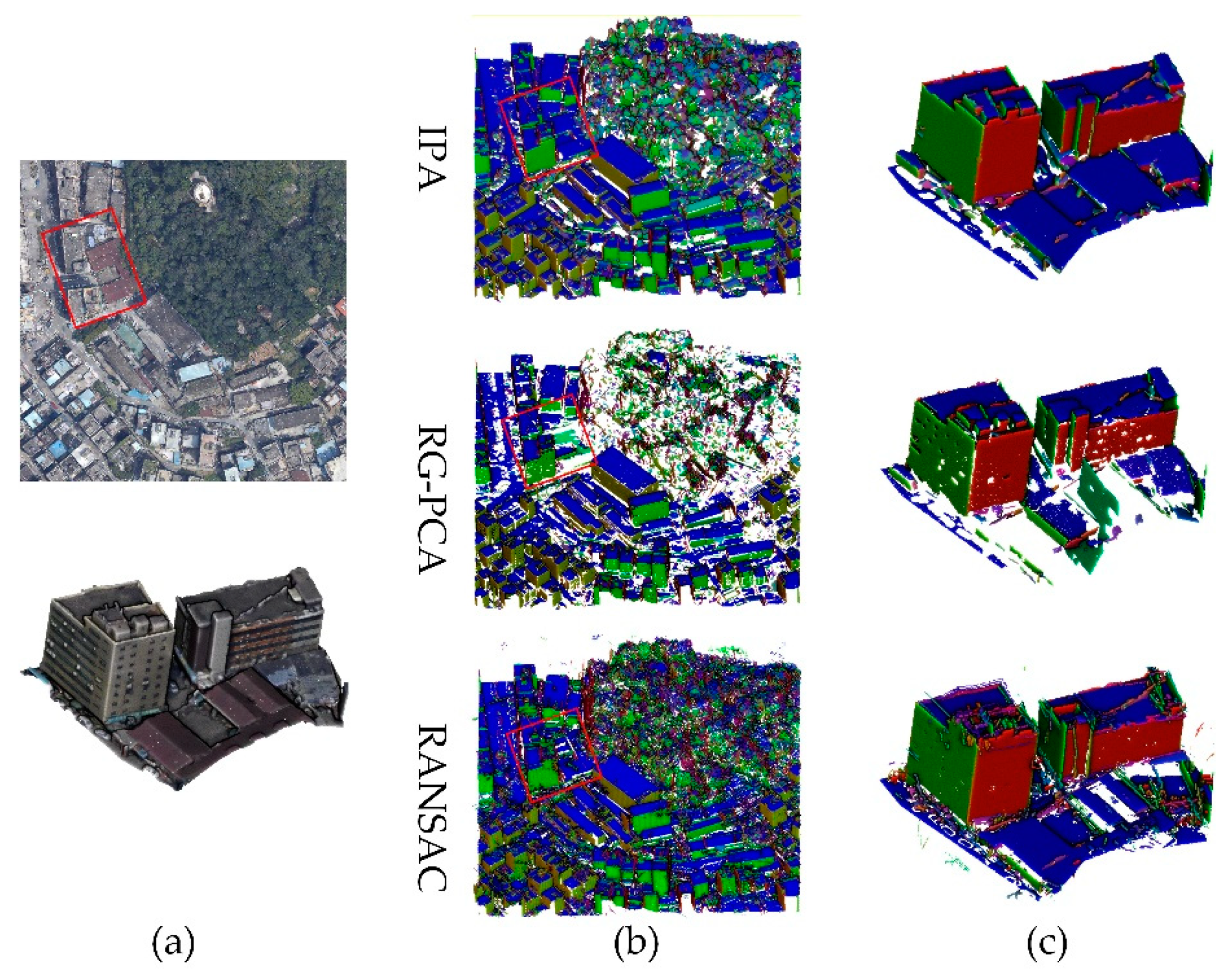
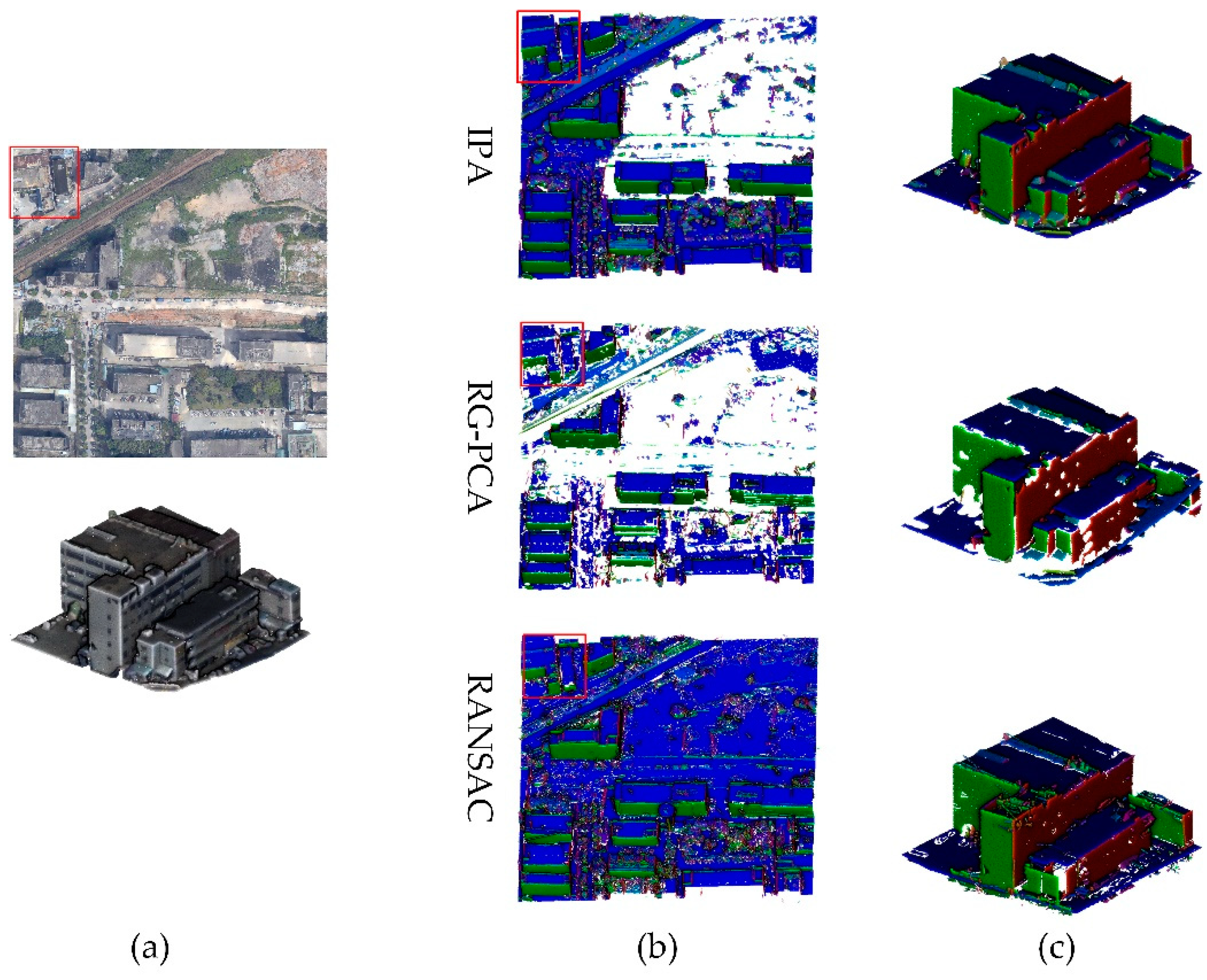
3.1.2. Evaluations of Large-Scale Tilewise Planar Extraction

Three tiles are chosen as the experimental data for the comparison experiments. First, because only the RG-PCA and RANSAC are scalable to process large scale datasets, and they are the most popular for extracting building planes, IPA is first compared with these methods for large-scale tilewise planar extraction, as shown in Figure 8, Figure 9 and Figure 10, respectively. For each tile, the subfigures in (a) show the original point clouds and the enlarged areas, and (b) and (c) show the plane extraction results, with points projected to the extracted plane, for the whole and enlarged areas, respectively. The performances in the three tiles are quite consistent for the three methods. It could be noted that for the small objects affiliated with a larger plane, the RG-PCA generally discards these points (i.e., the holes on the planes), and RANSAC detects them as individual objects, which is not the desired result. In addition, the RANSAC approach also ignores the connectivity constraint for planes (e.g., clustering distant points onto the same plane); on the other hand, RG-PCA explicitly enforces the neighbor connectivity in the extraction step. In addition, for large planes in the enlarged area of the three tiles, we also compute the completeness of the extracted points (i.e., projected area of the extracted points with the manually labelled reference, as shown in the captions for Figure 8, Figure 9 and Figure 10). The average completeness values for the three areas are 99.8%, 87.6%, and 98.3% for IPA, RG-PCA, and RANSAC, respectively.

In addition, for large planes in the enlarged area of the three tiles, three metrics (i.e., surface coverage, the number of small holes and the number of fragments) are used for qualitative evaluations. The average surface coverage (i.e., projected area of the extracted points with the manually labelled reference) for the three tiles are 99.8%, 87.6%, and 98.3% for IPA, RG-PCA and RANSAC, respectively. The numbers of small holes and fragments are counted and recorded in

Table 1. Qualitative evaluations for planar surface extraction results.

	Tile 1			Tile 2			Tile 3
methods	IPA	RG-PCA	RANSAC	IPA	RG-PCA	RANSAC	IPA	RG-PCA	RANSAC
number of small holes	3	69	29	15	172	43	2	46	24
number of fragments	9	10	106	44	39	287	13	11	137

. The numbers of fragments from IPA are close to that from RG-PCA, but the numbers of small holes from IPA are significantly smaller. Although RANSAC extracts more planes, it also produces more fragments, and the numbers of small holes are significantly larger than that of the IPA.

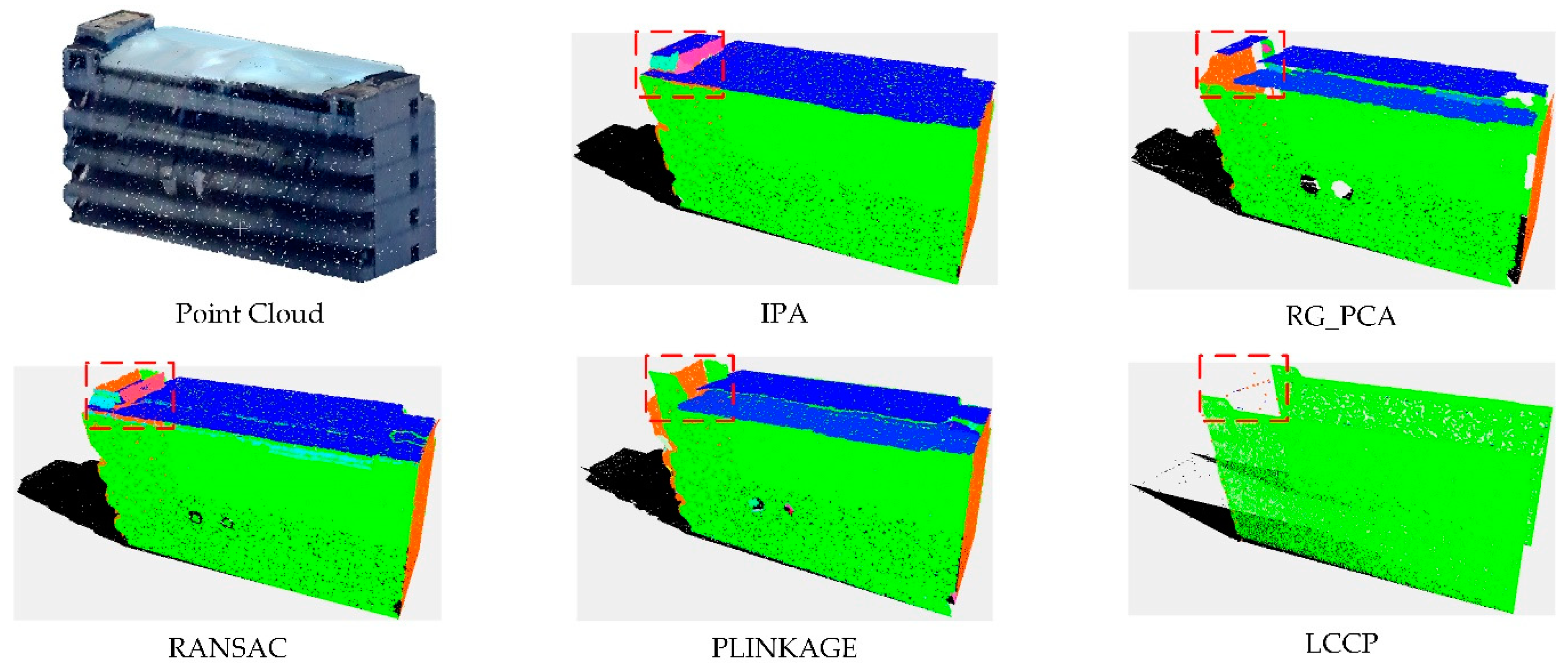
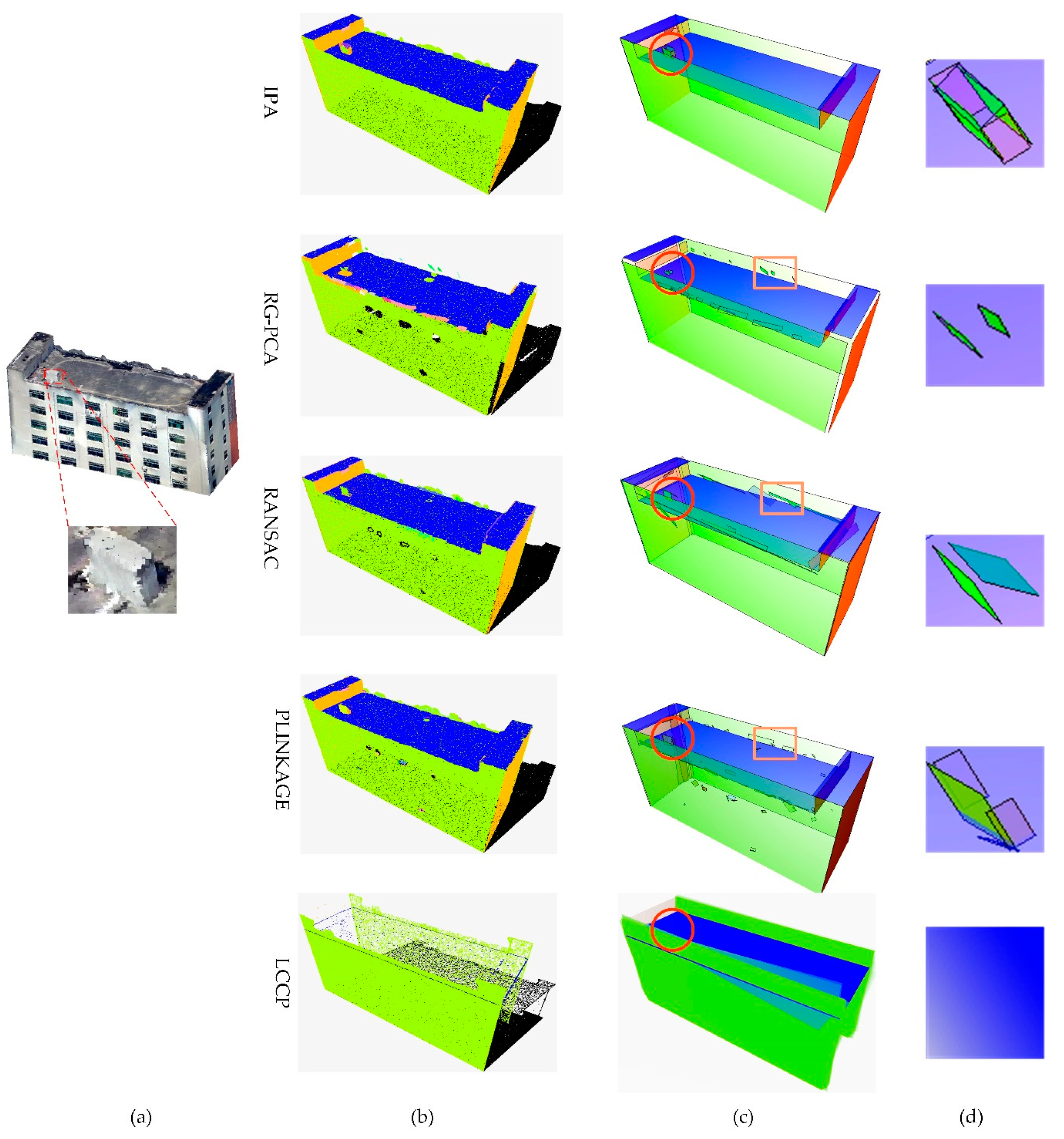
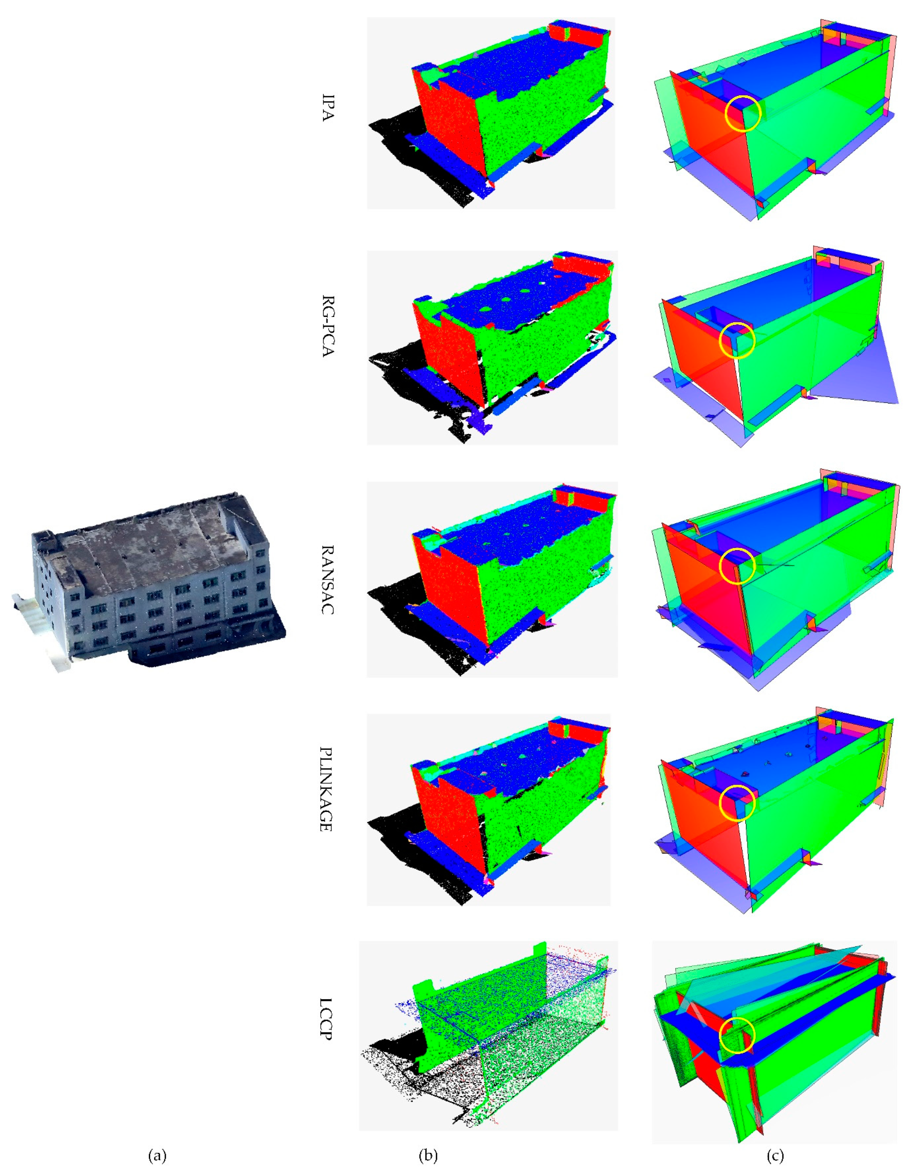
3.1.3. Evaluations of the Abstraction Quality of a Single Building

Three typical buildings are chosen from three tiles as experimental data. Building 1 has sharp features that are noticeably smoothed, which can test the ability to handle sharp features. Building 2 has detailed structures and deformations on planes to evaluate the effect of alleviating deformations, while, at the same time, retaining detailed structures. Building 3 has features of both difficulties of the above.

To evaluate the ability of detecting the point cloud buildings shapes, all tested methods are applied to extract the planes for building 1, and the results show the superiority of IPA regarding the completeness of the extracted planes. As shown in Figure 11, IPA can extract intact planar surfaces, while the sharp features are over-segmented or under-segmented by the other methods, especially in the marked region, where the sharp feature is smoothed. The normal vectors used in the comparison methods are estimated by local points. The RG-PCA extracts building planes based on the similarity among the normal vectors; however, at the smoothed sharp features, the normal vectors change continuously, which indicates that these parts cannot be extracted. RANSAC extracts building planes by model fitting, but this method is unsuitable for sharp features being extracted as curved surfaces or piecewise planes, while smoothed sharp features are expressed by curved surfaces. PLINKAGE uses a hierarchical clustering algorithm, which is able to process obvious sharp features, however, when the sharp features are smoothed by noise, the extracted planes may be under-segmented. The LCCP extracts the planes by region growing using the locally convex connected relationships of supervoxels, but the lack of noise processing and the retention of sharp features lead to many over-segmentations and under-segmentations in the segmentation results. In contrast, IPA estimates global normal vectors based on maximum planar support regions, where the cross-border regions almost never exist because of the constraint of planarity. Thus, by using the global normal vectors to distinguish sharp features, which ensures that the sharp features are not under-segmented or over-segmented, plane extraction with IPA is shown to be exact.

In general, it is difficult to avoid smoothing out a detailed structure, while processing noise. However, for accessory structures with obvious building features, IPA also has the ability to retain its structure as the marked region shown in Figure 12. In addition, for deformations on building surfaces caused by noise and appendages, IPA can abstract the intact planar surface without the influence of deformations, while there are fragmented planar extractions in the comparison methods, as shown in Figure 12c. For example, spurious faces caused by RANSAC can result in many fragmentation faces, as shown in rectangular marked region in Figure 12; PLINKAGE extracts deformations as independent planes, which also results in many fragmentations.

To evaluate the topology of the planar abstractions, all tested methods are applied to abstract the planes for building 3. As the marked region shown in Figure 13, planar abstraction from IPA can retain true direction and a tight relationship among adjacent planes. In contrast, there are many problems in planar abstraction results from other methods, such as the wrong direction of planes, the large gap between adjacent planes and the wrong adjacent planes. For RG-PCA, the poor ability of boundary handling makes points in sharp features cannot be assigned to corresponding planes, which creates a large gap between adjacent planes. For RANSAC, the spurious face generated between two planes which should be adjacent, changes the spatial relationship among these two adjacent planes during planar abstraction. For PLINKAGE, under-segmentation where multiple planes are segmented into one plane, makes the direction of abstracted plane deviates. In contrast, the global normal vectors from IPA are able to be distinguished in sharp features; therefore, the points in sharp features can be assigned to corresponding planes correctly, which makes the adjacent planes close together. In addition, without under-segmentation or over-segmentation, the abstracted planes from IPA are intact and continuous.

3.2. Quantitative Analysis

To quantitatively evaluate the accuracies of IPA, four metrics are employed. Completeness and Correctness [54] are used to evaluate the quality of the extracted planes. Completeness is represented by the percentage of correctly segmented planes compared to the number of reference planes. Correctness is equivalent to the percentage of the correctly segmented planes compared to the segmentation results:

$$Completeness=\frac{TP}{TP+FN}$$

(9)

$$Correctness=\frac{TP}{TP+FP}$$

(10)

where TP (true positive) represents the number of planes correctly segmented, FN (false negative) represents the number of planes missed and FP (false positive) represents the number of planes incorrectly segmented. The number of unassigned points(N_up) is used to assess the robustness to noise. The final metric used is points correctness(PC), which is defined as follows:

$$PC=\frac{P_{correctness}}{P_{total}}$$

(11)

where P_Correctness represents the number of points correctly segmented and P_total represents the total number of points.

We statistically analyzed our method, RG-PCA, LCCP and PLINKAGE. Considering that the number of points in the final result from PLINKAGE increases because of the interpolation involved, the value of N_up in PLINKAGE is not counted. The quantified indicators of the extracted planes are counted as shown in

Table 2. Statistical analysis of surface extraction results.

	Number of Points	Methods	Nup	TP	FN	FP
building 1	127,665	IPA	362	13	1	10
		RG-PCA	24,281	7	7	4
		RANSAC	4159	10	4	16
		LCCP	0	2	12	87
		PLINKAGE	/	9	5	35
building 2	278,893	IPA	227	15	0	0
		RG-PCA	19,323	10	5	10
		RANSAC	5705	11	4	22
		LCCP	0	2	13	106
		PLINKAGE	/	15	0	72
building 3	258,245	IPA	2356	24	0	22
		RG-PCA	30,553	17	7	29
		RANSAC	7805	23	3	26
		LCCP	0	3	21	397
		PLINKAGE	/	16	8	161

. For Building 1, the number of FP from our method is higher than that from RG-PCA. Because of the high noise level, many planes cannot be detected by the RG-PCA.

As shown in Figure 14, the statistical analysis indicated that the segmentation results of IPA outperform the counterparts. Because of the large amounts of noise and deformation present in the point cloud data of Building 1 and Building 3, many of the points are unrecognized. Hence, a significant difference is observed between the N_up values of the different segmentation methods. Moreover, over-segmentation caused by noise results in low Completeness and Correctness values for the RG-PCA. IPA maintains a high completeness rate, but the correction peak is approximately 50%. The errors in the results from IPA are mainly located at sharp features with serious deformation. For all three buildings tested, the time cost of IPA is acceptable as shown in Figure 14.

4. Conclusions

Recent advances in MVS techniques and the new popularity of penta-view aerial oblique images have led to a revolution, which appears to have prompted a renaissance in three-dimensional reconstruction by photogrammetry. However, the noise inherent in photogrammetric point clouds has impeded the development of novel applications (e.g., building reconstruction and city scene representation). In the present study, we use optimization techniques to refine the normal vectors of photogrammetric point clouds by hierarchical clustering and careful handling of object boundaries. The normal vectors are not only robust to the noise in the plane, but also maintain sharp features. In combination with region-growing, integrated planes can be segmented accurately and efficiently. Since the proposed method can achieve strong robustness, almost all of the major planes of a building can be extracted; thus, the planar abstraction of a building can be produced from oblique images. These planar abstractions will be exploited further in the future for automatic or interactive building reconstruction methods. Furthermore, extraction of arbitrary geometrical primitives (e.g., spheres, cylinders, and cones), rather than planes, will also be investigated.

References

1. Haala, N.; Rothermel, M.; Cavegn, S. Extracting 3D urban models from oblique aerial images. In Proceedings of the IEEE in Urban Remote Sensing Event (JURSE), Lausanne, Switzerland, 30 March–1 April 2015. [Google Scholar]
2. Hu, H.; Zhu, Q.; Du, Z.; Zhang, Y.; Ding, Y. Reliable spatial relationship constrained feature point matching of oblique aerial images. Photogramm. Eng. Remote Sens. 2015, 81, 49–58. [Google Scholar] [CrossRef]
3. Gerke, M.; Nex, F.; Remondino, F.; Jacobsen, K.; Kremer, J.; Karel, W.; Huf, H.; Ostrowski, W. Orientation of oblique airborne image sets-experiences from the ISPRS/EUROSDR benchmark on multi-platform photogrammetry. Int. Arch. Photogramm. Remote Sens. Spat. Inf. Sci. 2016, 41, 185–191. [Google Scholar] [CrossRef]
4. Xie, L.; Hu, H.; Wang, J.; Zhu, Q.; Chen, M. An asymmetric re-weighting method for the precision combined bundle adjustment of aerial oblique images. ISPRS J. Photogram. Remote Sens. 2016, 117, 92–107. [Google Scholar] [CrossRef]
5. Koci, J.; Jarihani, B.; Leon, J.X.; Sidle, R.C.; Wilkinson, S.N.; Bartley, R. Assessment of UAV and ground-based Structure from Motion with multi-view stereo photogrammetry in a gullied savanna catchment. ISPRS Int. J. Geo-Inf. 2017, 6, 328. [Google Scholar] [CrossRef]
6. Remondino, F.; Spera, M.G.; Nocerino, E.; Menna, F.; Nex, F. State of the art in high density image matching. Photogramm. Rec. 2014, 29, 144–166. [Google Scholar] [CrossRef]
7. Xiong, B.; Elberink, S.O.; Vosselman, G. Building modeling from noisy photogrammetric point clouds. ISPRS Ann. Photogramm. Remote Sens. Spat. Inf. Sci. 2014, 1, 197–204. [Google Scholar] [CrossRef]
8. Guerrero, P.; Kleiman, Y.; Ovsjanikov, M.; Mitra, N.J. PCPNet Learning Local Shape Properties from Raw Point Clouds. Comput. Graph. Forum 2018, 37, 75–85. [Google Scholar] [CrossRef] [Green Version]
9. Boulch, A.; Marlet, R. Deep learning for robust normal estimation in unstructured point clouds. Comput. Graph. Forum 2016, 35, 281–290. [Google Scholar] [CrossRef]
10. Muja, M.; Lowe, D.G. Scalable nearest neighbor algorithms for high dimensional data. IEEE Trans. Pattern Anal. Mach. Intell. 2014, 36, 2227–2240. [Google Scholar] [CrossRef] [PubMed]
11. Huang, H.; Li, D.; Zhang, H.; Ascher, H.; Cohen-Or, D. Consolidation of unorganized point clouds for surface reconstruction. ACM Trans. Graph. 2009, 28, 176. [Google Scholar] [CrossRef]
12. Kalogerakis, E.; Nowrouzezahrai, D.; Simari, P.; Singh, K. Extracting lines of curvature from noisy point clouds. Comput.-Aided Des. 2009, 41, 282–292. [Google Scholar] [CrossRef] [Green Version]
13. Lee, W.; Park, J.; Kim, J.; Kim, W.; Yu, C. New approach to accuracy verification of 3D surface models: An analysis of point cloud coordinates. J. Prosthodont. Res. 2016, 60, 98–105. [Google Scholar] [CrossRef] [PubMed]
14. Lin, C.; Chen, J.; Su, P.; Chen, C. Eigen-feature analysis of weighted covariance matrices for LiDAR point cloud classification. ISPRS J. Photogramm. Remote Sens. 2014, 94, 70–79. [Google Scholar] [CrossRef]
15. Cazals, F.; Pouget, M. Estimating differential quantities using polynomial fitting of osculating jets. Comput. Aided Geom. Des. 2005, 22, 121–146. [Google Scholar] [CrossRef] [Green Version]
16. Dimitrov, A.; Gu, R.; Golparvar Fard, M. Non-Uniform B-Spline Surface Fitting from Unordered 3D Point Clouds for As-Built Modeling. Comput.-Aided Civ. Infrastruct. Eng. 2016, 31, 483–498. [Google Scholar] [CrossRef]
17. Li, L.; Yang, F.; Zhu, H.; Li, D.; Li, Y.; Tang, L. An improved RANSAC for 3D point cloud plane segmentation based on normal distribution transformation cells. Remote Sens. 2017, 9, 433. [Google Scholar] [CrossRef]
18. Chen, D.; Zhang, L.; Mathiopoulos, P.T.; Huang, X. A methodology for automated segmentation and reconstruction of urban 3-D buildings from ALS point clouds. IEEE J. Sel. Top. Appl. Earth Obs. Remote Sens. 2014, 7, 4199–4217. [Google Scholar] [CrossRef]
19. Hulik, R.; Spanel, M.; Smrz, P.; Materna, Z. Continuous plane detection in point-cloud data based on 3D Hough Transform. J. Vis. Commun. Image Represent. 2014, 25, 86–97. [Google Scholar] [CrossRef]
20. Limberger, F.A.; Oliveira, M.M. Oliveira, Real-time detection of planar regions in unorganized point clouds. Pattern Recognit. 2015, 48, 2043–2053. [Google Scholar] [CrossRef]
21. Wang, Y.; Zhu, X. Automatic feature-based geometric fusion of multiview TomoSAR point clouds in urban area. IEEE J. Sel. Top. Appl. Earth Obs. Remote Sens. 2015, 8, 953–965. [Google Scholar] [CrossRef]
22. Tarsha-Kurdi, F.; Landes, T.; Grussenmeyer, P. Hough-transform and extended ransac algorithms for automatic detection of 3D building roof planes from lidar data. In Proceedings of the ISPRS Workshop on Laser Scanning, Espoo, Finland, 12–14 September 2007. [Google Scholar]
23. Yan, J.; Shan, J.; Jiang, W. A global optimization approach to roof segmentation from airborne lidar point clouds. ISPRS J. Photogramm. Remote Sens. 2014, 94, 183–193. [Google Scholar] [CrossRef]
24. Schnabel, R.; Wahl, R.; Klein, R. Efficient RANSAC for point-cloud shape detection. Comput. Graph. Forum 2007, 26, 214–226. [Google Scholar] [CrossRef]
25. Yu, Y.; Wu, Q.; Khan, Y.; Chen, M. An adaptive variation model for point cloud normal computation. Neural Comput. Appl. 2015, 26, 1451–1460. [Google Scholar] [CrossRef]
26. Rabbani, T.; Van Den Heuvel, F.; Vosselmann, G. Segmentation of point clouds using smoothness constraint. Int. Arch. Photogramm. Remote Sens. Spat. Inf. Sci. 2006, 36, 248–253. [Google Scholar]
27. He, M.; Cheng, Y.; Nie, Y.; Zhao, Z.; Zhang, F. An Algorithm of Combining Delaunay TIN Models and Region Growing for Buildings Extraction. In Proceedings of the International Conference on Computer Science and Technology, Guilin, China, 25–29 July 2017. [Google Scholar]
28. Xu, Y.; Yao, W.; Hoegner, L.; Stilla, U. Segmentation of building roofs from airborne LiDAR point clouds using robust voxel-based region growing. Remote Sens. Lett. 2017, 8, 1062–1071. [Google Scholar] [CrossRef]
29. Nurunnabi, A.; West, G.; Belton, D. Outlier detection and robust normal-curvature estimation in mobile laser scanning 3D point cloud data. Pattern Recognit. 2015, 48, 1404–1419. [Google Scholar] [CrossRef]
30. Qin, L.; Wu, W.; Tian, Y.; Xu, W. Lidar filtering of urban areas with region growing based on moving-window weighted iterative least-squares fitting. IEEE Geosci. Remote Sens. Lett. 2017, 14, 841–845. [Google Scholar] [CrossRef]
31. Amini Amirkolaee, H.; Arefi, H. 3D Semantic Labeling using Region Growing Segmentation Based on Structural and Geometric Attributes. J. Geomat. Sci. Technol. 2017, 7, 1–16. [Google Scholar]
32. Guo, B.; Li, Q.; Huang, X.; Wang, C. An improved method for power-line reconstruction from point cloud data. Remote Sens. 2016, 8, 36. [Google Scholar] [CrossRef]
33. Tseng, Y.; Tang, K.; Chou, F. Surface reconstruction from LiDAR data with extended snake theory. In Proceedings of the International Workshop on Energy Minimization Methods in Computer Vision and Pattern Recognition, Ezhou, China, 27–29 August 2007. [Google Scholar]
34. Cgal. Available online: https://doc.cgal.org/latest/Point_set_shape_detection_3/index.html (accessed on 5 August 2018).
35. Lin, Y.; Wang, C.; Zhai, D.; Li, W.; Li, J. Toward better boundary preserved supervoxel segmentation for 3D point clouds. ISPRS J. Photogramm. Remote Sens. 2018, 143, 39–47. [Google Scholar] [CrossRef]
36. Papon, J.; Abramov, A.; Schoeler, M.; Worgotter, F. Voxel cloud connectivity segmentation-supervoxels for point clouds. In Proceedings of the IEEE Conference on Computer Vision and Pattern Recognition, Portland, OR, USA, 23–28 Jun 2013. [Google Scholar]
37. Wang, H.; Wang, C.; Luo, H. 3-D point cloud object detection based on supervoxel neighborhood with Hough forest framework. IEEE J. Sel. Top. Appl. Earth Obs. Remote Sens. 2015, 8, 1570–1581. [Google Scholar] [CrossRef]
38. Zhu, Q.; Li, Y.; Hu, H.; Wu, B. Robust point cloud classification based on multi-level semantic relationships for urban scenes. ISPRS J. Photogramm. Remote Sens. 2017, 129, 86–102. [Google Scholar] [CrossRef]
39. Dong, Z.; Yang, B.; Hu, P.; Scherer, S. An efficient global energy optimization approach for robust 3D plane segmentation of point clouds. ISPRS J. Photogramm. Remote Sens. 2018, 137, 112–133. [Google Scholar] [CrossRef]
40. Rusu, R.B.; Cousins, S. 3D is here: Point cloud library (PCL). In Proceedings of the IEEE International Conference on Robotics and automation (ICRA), Shanghai, China, 11–13 October 2011. [Google Scholar]
41. Kong, T.Y.; Rosenfeld, A. Digital topology: Introduction and survey. Comput. Vis. Graph. Image Process. 1989, 48, 357–393. [Google Scholar] [CrossRef]
42. Rusu, R.B.; Blodow, N.; Beetz, M. Fast point feature histograms (FPFH) for 3D registration. In Proceedings of the IEEE International Conference on Robotics and Automation (ICRA’092009), Kobe, Japan, 12–17 May 2009. [Google Scholar]
43. Matei, B.C.; Sawhney, H.S.; Samarasekera, S.; Kim, J.; Kumar, R. Building segmentation for densely built urban regions using aerial lidar data. In Proceedings of the IEEE Conference on Computer Vision and Pattern Recognition, Anchorage, AK, USA, 23–28 June 2008. [Google Scholar]
44. Ramón, M.J.; Pueyo, E.L.; Oliva-Urcia, B.; Larrasoaña, J.C. Virtual directions in paleomagnetism: A global and rapid approach to evaluate the NRM components. Front. Earth Sci. 2017, 5, 8. [Google Scholar] [CrossRef]
45. Vo, A.; Truong-Hong, L.; Laefer, D.F.; Bertolotto, M. Octree-based region growing for point cloud segmentation. ISPRS J. Photogramm. Remote Sens. 2015, 104, 88–100. [Google Scholar] [CrossRef]
46. Avron, H.; Sharf, A.; Greif, C.; Cohen-Or, D. ℓ 1-Sparse reconstruction of sharp point set surfaces. ACM Trans. Graph. 2010, 29, 135. [Google Scholar] [CrossRef]
47. Belongie, S. “Rodrigues’ Rotation Formula.” From MathWorld—A Wolfram Web Resource, Created by Eric W. Weisstein. Available online: http://mathworld.wolfram.com/RodriguesRotationFormula.html (accessed on 17 October 2018).
48. Friedman, J.; Hastie, T.; Tibshirani, R. The Elements of Statistical Learning; Springer: Berlin, Germany, 2001; Volume 1. [Google Scholar]
49. Hu, H.; Ding, Y.; Zhu, Q.; Wu, B.; Xie, L.; Chen, M. Stable least-squares matching for oblique images using bound constrained optimization and a robust loss function. ISPRS J. Photogramm. Remote Sens. 2016, 118, 53–67. [Google Scholar] [CrossRef]
50. Pukelsheim, F. The three sigma rule. Am. Stat. 1994, 48, 88–91. [Google Scholar]
51. Agarwal, S.; Mierle, K. Ceres Solver. 2013. Available online: https://github.com/ceres-solver/ceres-solver (accessed on 5 May 2018).
52. Stein, S.C.; Schoeler, M.; Papon, J.; Wörgötter, F. Object Partitioning Using Local Convexity. In Proceedings of the IEEE Conference on Computer Vision and Pattern Recognition, Columbus, OH, USA, 23–28 June 2014. [Google Scholar]
53. Lu, X.; Yao, J.; Tu, J.; Li, K.; Li, L.; Liu, Y. Pairwise linkage for point cloud segmentation. ISPRS Ann. Photogramm. Remote Sens. Spat. Inf. Sci. 2016, 3, 201–208. [Google Scholar]
54. Chen, Y.; Cheng, L.; Li, M.; Wang, J.; Tong, L.; Yang, K. Multiscale grid method for detection and reconstruction of building roofs from airborne LiDAR data. IEEE J. Sel. Top. Appl. Earth Obs. Remote Sens. 2014, 7, 4081–4094. [Google Scholar] [CrossRef]
Figure 1. Different region selection and geometric kernel for normal estimation. Principal component analysis (PCA) (a), jet fitting (b) and MLS Sphere fitting (c) generally use local regions, and select planes, quadratic surfaces, and spheres as the geometric kernel, respectively. In addition, the geometric kernel can also be learned from exemplar datasets (d). However, for noisy photogrammetric point clouds in urban environments, a large context should be selected to keep sharp features, such as the sharp edges of a building.
Ijgi 07 00431 g001
Figure 2. Processing pipeline of the proposed method.
Ijgi 07 00431 g002
Figure 3. Directional expansion of the maximal support regions. (a) Photogrammetric point cloud, (b) supervoxels, (c) growing region of a supervoxel located in a plane, and (d) growing region of a supervoxel located in a sharp feature.
Ijgi 07 00431 g003
Figure 4. Constraints used during region growing of the support region. (a) Planarity constraint determined from the spectral features. (b) Angle deviation in the supervoxels.
Ijgi 07 00431 g004
Figure 5. Mutual validation of the connectivity test. The dots represent supervoxels and the rounded rectangles represent support regions. (a) Only one side of the region is contained, cjSi but ci Sj. (b) The shaded dots are mutually contained, ciSj and cjSi.
Ijgi 07 00431 g005
Figure 6. Visualization of normal vectors. (a) shows a cube model with 240,000 points. (c) shows the same model but with 0.5% noise. (b,d) show the results from the proposed method, the RMSE are 0.0022 and 0.0231 respectively. (c,f) show the results estimated by local information only, the RMSE are 0.0707 and 0.433 respectively. The proposed method produces more consistent normal vectors.
Ijgi 07 00431 g006
Figure 7. Normal vectors visualization. The left column represents photogrammetric point clouds, the middle column represents normal vectors optimized by IPA, and the right column represents initial normal vectors estimated by the PCA.
Ijgi 07 00431 g007
Figure 8. Comparison of planar surface extraction from the point cloud of tile 1.
Ijgi 07 00431 g008
Figure 9. Comparison of planar surface extraction from the point cloud of tile 2.
Ijgi 07 00431 g009
Figure 10. Comparison of planar surface extraction from the point cloud of tile 3.
Ijgi 07 00431 g010
Figure 11. Comparison of the planar abstraction quality of building 1.
Ijgi 07 00431 g011
Figure 12. Comparison of the planar abstraction quality of building 2. (a) Building point cloud, (b) planar abstractions, (c) extracted planes approximated by a set of planar polygons, and (d) magnified images of the circle marked regions in (c).
Ijgi 07 00431 g012
Figure 13. Comparison of the planar abstraction quality of building 3. (a) Building point cloud, (b) planar abstractions, and (c) extracted planes approximated by a set of planar polygons.
Ijgi 07 00431 g013
Figure 14. Efficiency analysis of algorithms.
Ijgi 07 00431 g014