Study of a Gray Genetic BP Neural Network Model in Fault Monitoring and a Diagnosis System for Dam Safety


Abstract
:1. Introduction
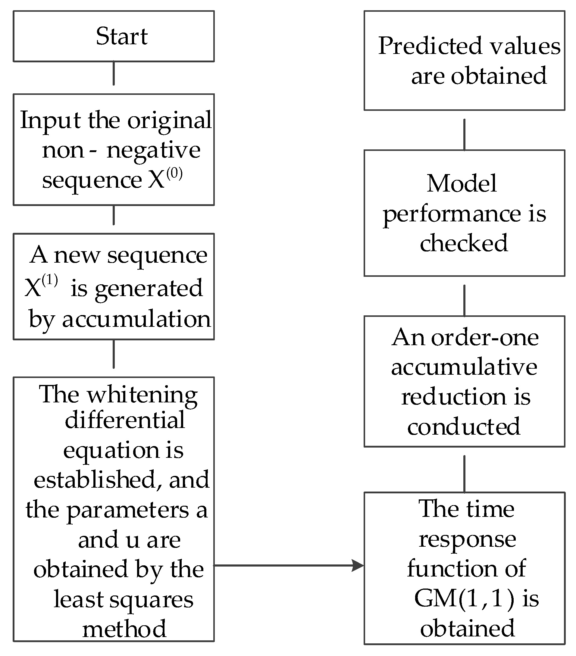
- (1)
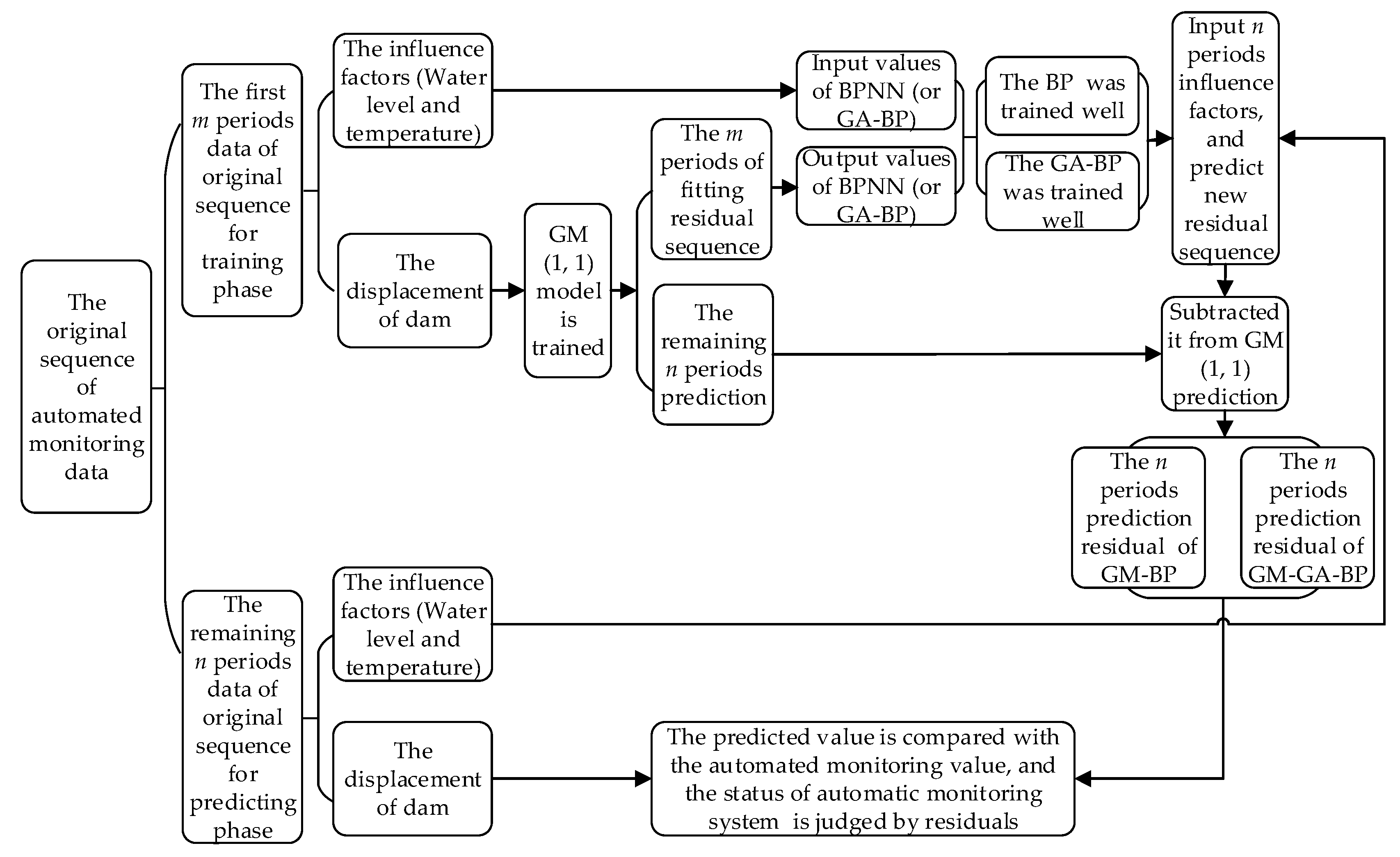
- The GM (1, 1) was used to fit and predict the automated monitoring sequences, resulting in the fitting value and the predicted value. The fitting value and the predicted value represent the main trend of the dam, and their values are reliable and almost linear.
- (2)
- The residual sequences of the GM (1, 1) can be obtained by subtracting the original values from the predicted values. The residual sequences reflect the volatility of the dam, and their values are unstable and non-linear.
- (3)
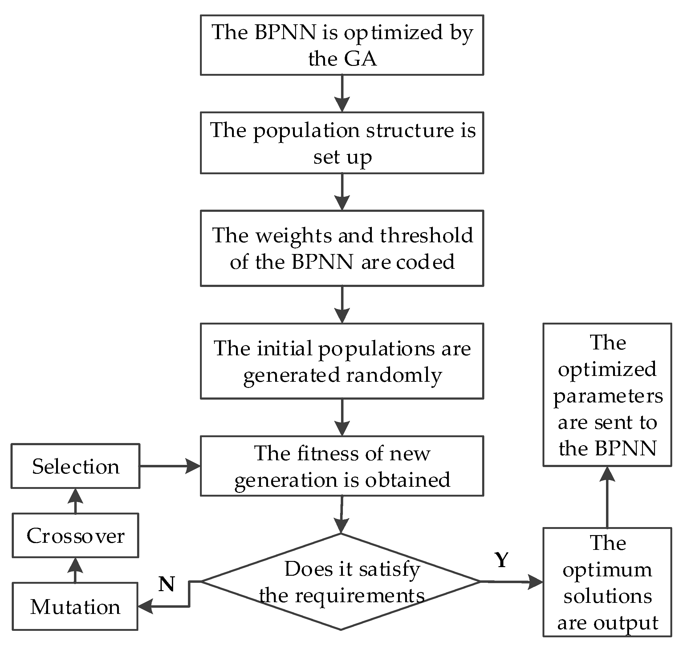
- The GA is used to optimize the structure of the BPNN, and the GA-BP is built.
- (4)
- The GA-BP is trained by the influence factors (water level and temperature) and the residual values of the GM (1, 1): the input values of the GA-BP model are the influencing factors, and the output values are the residual values of the GM (1, 1).
- (5)
- The GA-BP is found to be trained well and can be adopted to predict new residuals; when the influencing factors (water level and temperature) are entered, the model will output the new residuals.
- (6)
- The dam displacement prediction is obtained by subtracting the new residuals from the prediction of the GM (1, 1).
2. Model Principles
2.1. Modeling with a GM
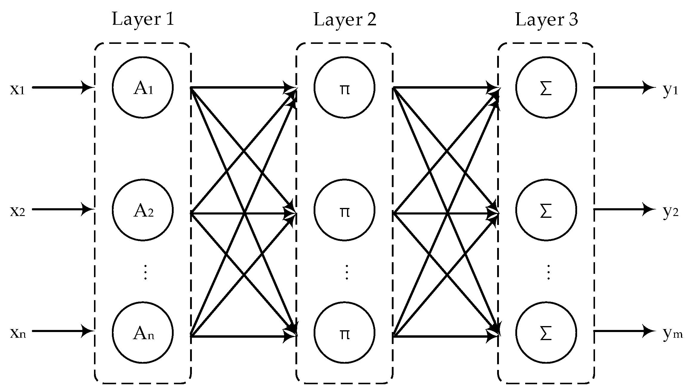
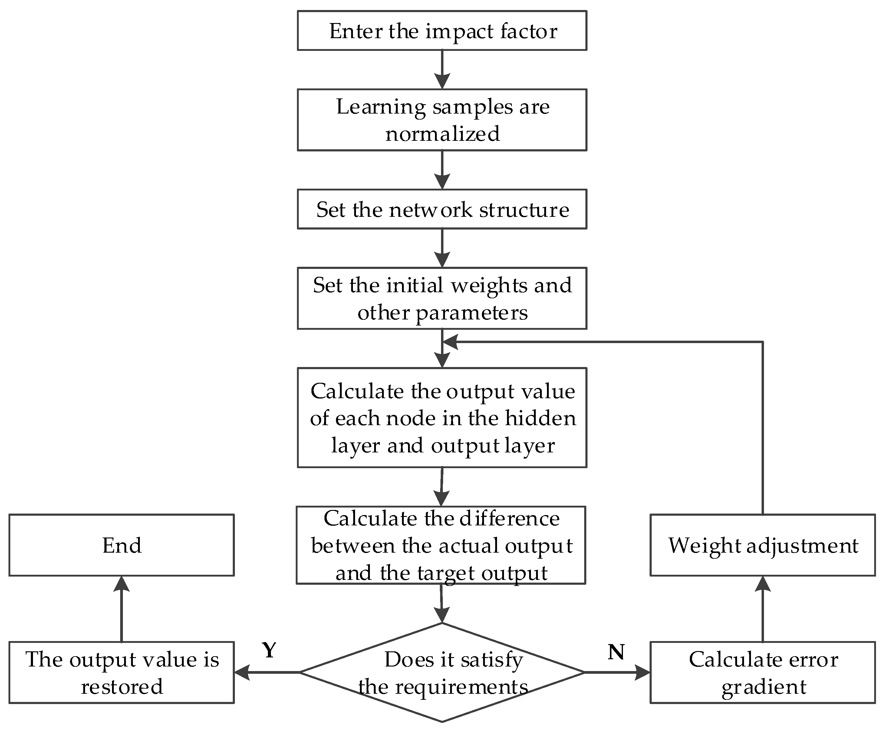
2.2. Modeling with the BPNN Model
2.3. Modeling with the GA-BP Model
2.4. Modeling with the GM-BP Model and GM-GA-BP Model
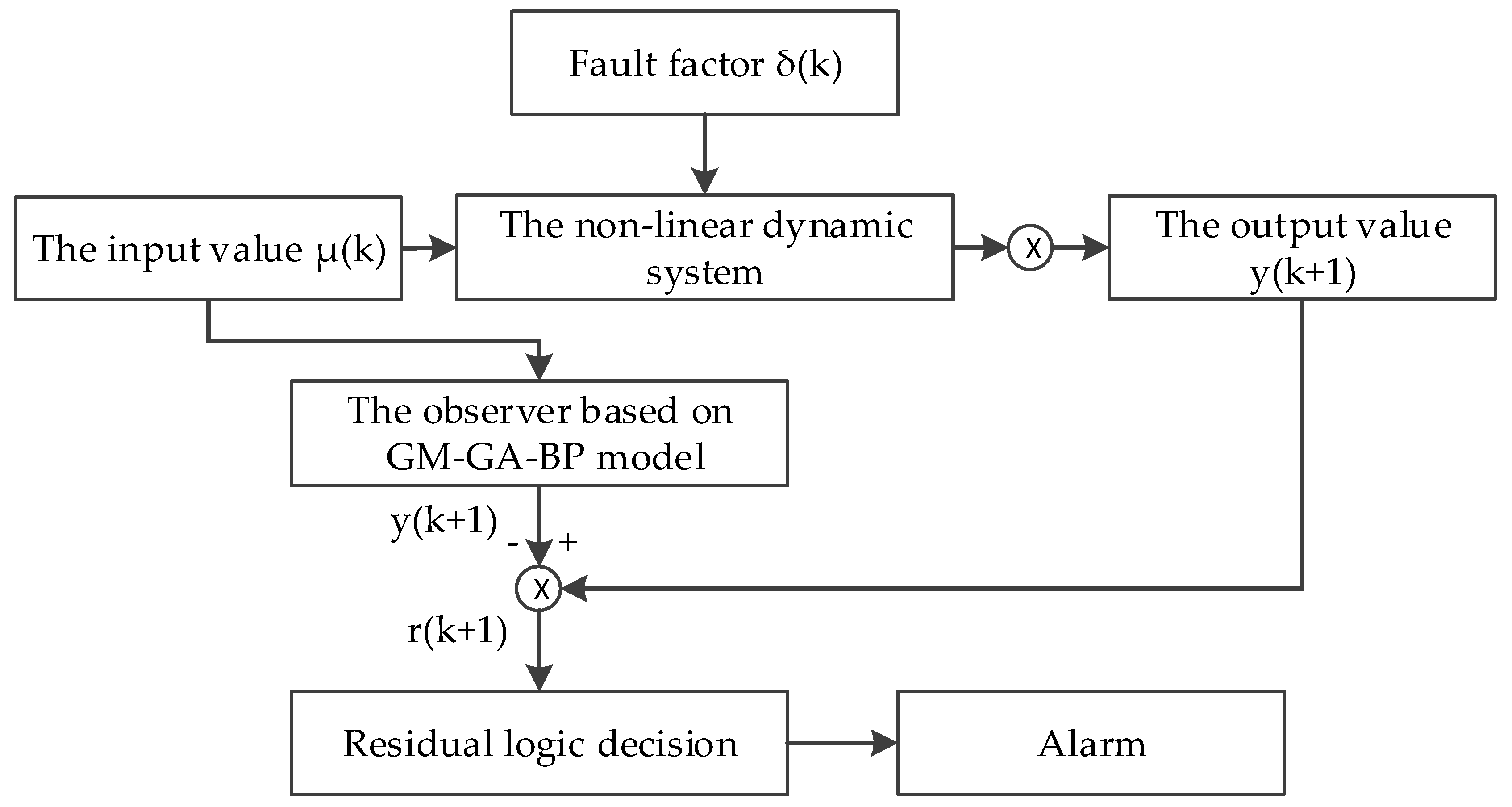
2.5. Design of a Dam Safety Fault Monitoring and Diagnosis System
3. Validation and Comparison of Model Performances
3.1. Setting of Model Parameters
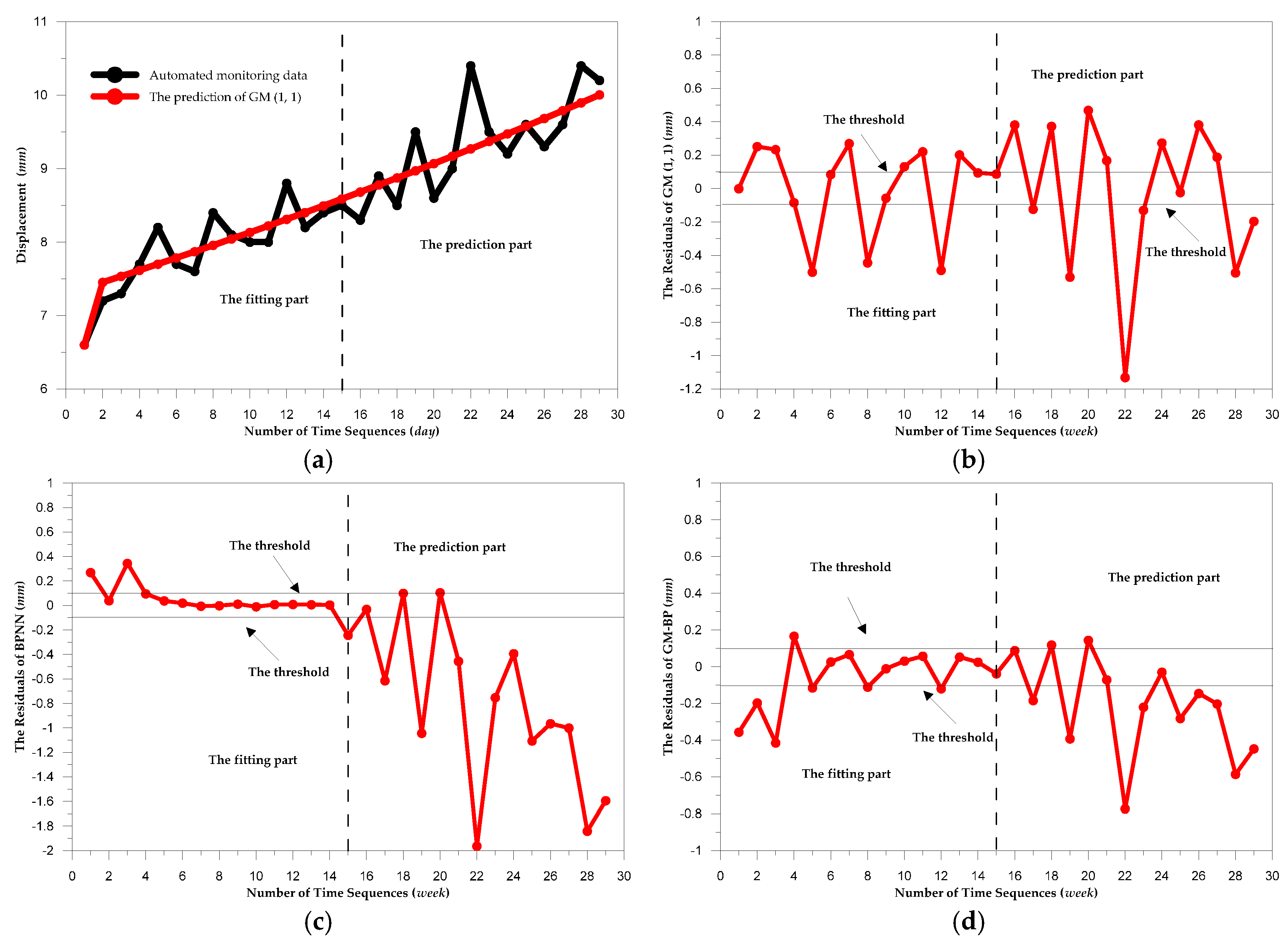
3.2. Analysis of the Models for Predicting the Displacement of Dam Deformation
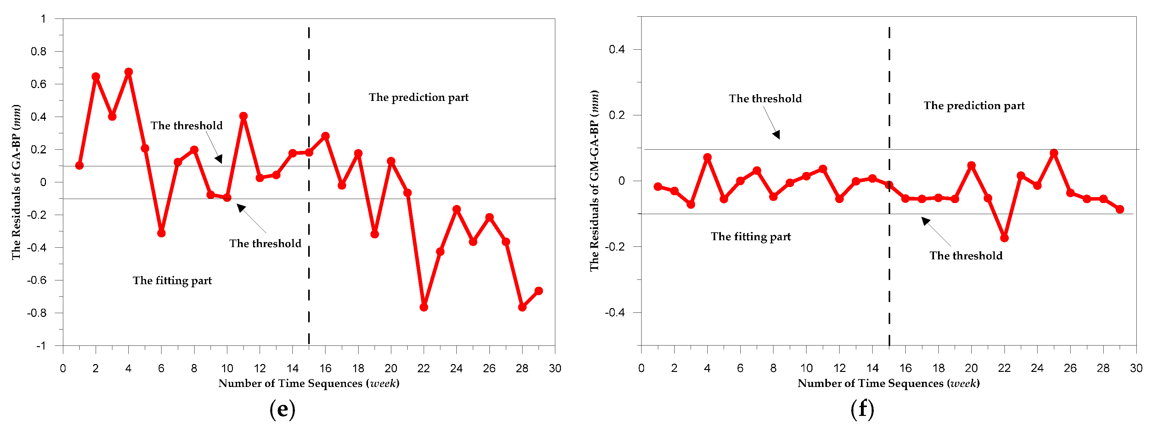
3.3. Evaluation for the Models
- (1)
- The MAE is calculated using the following formula:
- (2)
- The RMSE is calculated using the following formula:where Yt represents the actual deformation values from dam monitoring, represents the deformation prediction values of the model, and n represents the number of monitoring periods.
4. Conclusions
Acknowledgments
Author Contributions
Conflicts of Interest
References
- Dai, W.J.; Liu, N.; Santerre, R.; Pan, J.B. Dam Deformation Monitoring Data Analysis Using Space-Time Kalman Filter. ISPRS Int. J. Geo-Inf. 2016, 5, 236. [Google Scholar] [CrossRef]
- Gamse, S.; Zhou, W.H.; Tan, F.; Yuen, K.V.; Oberguggenberger, M. Hydrostatic-season-time model updating using Bayesian model class selection. Reliab. Eng. Syst. Saf. 2018, 169, 40–50. [Google Scholar] [CrossRef]
- Saidi, S.; Houimli, H.; Zid, J. Geodetic and GIS tools for dam safety: Case of Sidi Salem dam (northern Tunisia). Arab. J. Geosci. 2017, 10, 505. [Google Scholar] [CrossRef]
- Majdi, A.; Beiki, M. Evolving neural network using a genetic algorithm for predicting the deformation modulus of rock masses. Int. J. Rock Mech. Min. Sci. 2010, 47, 246–253. [Google Scholar] [CrossRef]
- Salazar, F.; Toledo, M.Á.; González, J.M.; Oñate, E. Early detection of anomalies in dam performance: A methodology based on boosted regression trees. Struct. Control Health Monit. 2017, 24, e2012. [Google Scholar] [CrossRef]
- Su, H.; Li, H.; Chen, Z.; Wen, Z. An approach using ensemble empirical mode decomposition to remove noise from prototypical observations on dam safety. SpringerPlus 2016, 5, 650. [Google Scholar] [CrossRef] [PubMed]
- Su, H.; Chen, Z.; Wen, Z. Performance improvement method of support vector machine-based model monitoring dam safety. Struct. Control Health Monit. 2016, 23, 252–266. [Google Scholar] [CrossRef]
- Tasci, L.; Kose, E. Deformation Forecasting Based on Multi Variable Grey Prediction Models. J. Grey Syst. 2016, 28, 56–64. [Google Scholar]
- Rocha, M. A quantitative method for the interpretation of the results of the observation of dams. In Proceedings of the 6th Congress on Large Dams, New York, NY, USA, 15–20 September 1958. [Google Scholar]
- Xerez, A.C.; Lamas, J.F. Methods of analysis of arch dam behavior. In Proceedings of the 6th Congress on Large Dams, New York, NY, USA, 15–20 September 1958; pp. 407–431. [Google Scholar]
- Pramthawee, P.; Jongpradist, P.; Sukkarak, R. Integration of creep into a modified hardening soil model for time-dependent analysis of a high rockfill dam. Comput. Geotech. 2017, 91, 104–116. [Google Scholar] [CrossRef]
- Costa, V.; Fernandes, W. Bayesian estimation of extreme flood quantiles using a rainfall-runoff model and a stochastic daily rainfall generator. J. Hydrol. 2017, 554, 137–154. [Google Scholar] [CrossRef]
- Akpinar, M.; Yumusak, N. Year Ahead Demand Forecast of City Natural Gas Using Seasonal Time Series Methods. Energies 2016, 9, 727. [Google Scholar] [CrossRef]
- Frank, R.J.; Davey, N.; Hunt, S.P. Time Series Prediction and Neural Networks. J. Intell. Robot. Syst. 2001, 31, 91–103. [Google Scholar] [CrossRef]
- Gan, L.; Shen, X.; Zhang, H. New deformation back analysis method for the creep model parameters using finite element nonlinear method. Cluster Comput. 2017, 20, 3225–3236. [Google Scholar] [CrossRef]
- Luo, G.; Hu, X.; Bowman, E.T.; Liang, J. Stability evaluation and prediction of the Dongla reactivated ancient landslide as well as emergency mitigation for the Dongla Bridge. Landslides 2017, 14, 1403–1418. [Google Scholar] [CrossRef]
- Fotopoulou, S.D.; Pitilakis, K.D. Predictive relationships for seismically induced slope displacements using numerical analysis results. Bull. Earthq. Eng. 2015, 13, 3207–3238. [Google Scholar] [CrossRef]
- Pal, M.; Mather, P.M. Support vector machines for classification in remote sensing. Int. J. Remote Sens. 2005, 26, 1007–1011. [Google Scholar] [CrossRef]
- Fan, F.M.; Collischonn, W.; Quiroz, K.J.; Sorribas, M.V.; Buarque, D.C.; Siqueira, V.A. Flood forecasting on the Tocantins River using ensemble rainfall forecasts and real-time satellite rainfall estimates. J. Flood Risk Manag. 2016, 9, 278–288. [Google Scholar] [CrossRef]
- Ju-Long, D. Control problems of grey systems. Syst. Control Lett. 1982, 1, 288–294. [Google Scholar] [CrossRef]
- Ju-Long, D. Introduction to grey system theory. J. Grey Syst. 1989, 1, 1–24. [Google Scholar]
- Salazar, F.; Toledo, M.A.; Oñate, E.; Morán, R. An empirical comparison of machine learning techniques for dam behaviour modelling. Struct. Saf. 2015, 56, 9–17. [Google Scholar] [CrossRef] [Green Version]
- Dal Sasso, S.F.; Sole, A.; Pascale, S.; Sdao, F.; Bateman Pinzón, A.; Medina, V. Assessment methodology for the prediction of landslide dam hazard. Nat. Hazards Earth Syst. Sci. 2014, 14, 557–567. [Google Scholar] [CrossRef] [Green Version]
- Ilić, S.A.; Vukmirović, S.M.; Erdeljan, A.M.; Kulić, F.J. Hybrid artificial neural network system for short-term load forecasting. Therm. Sci. 2012, 16, 215–224. [Google Scholar] [CrossRef]
- Rojek, I.; Jagodziński, M. Hybrid artificial intelligence system in constraint based scheduling of integrated manufacturing ERP systems. Hybrid Artif. Intell. Syst. 2012, 2, 229–240. [Google Scholar]
- Leccese, F. Subharmonics Determination Method based on Binary Successive Approximation Feed Forward Artificial Neural Network: A preliminary study. In Proceedings of the 9th IEEE International Conference on Environment and Electrical Engineering (EEEIC 2010), Prague, Czech Republic, 16–19 May 2010; pp. 442–446. [Google Scholar]
- Caciotta, M.; Giarnetti, S.; Leccese, F. Hybrid neural network system for electric load forecasting of telecomunication station. In Proceedings of the XIX IMEKO World Congress Fundamental and Applied Metrology, Lisbon, Portugal, 6–11 September 2009; Publishing House of Poznan University of Technology: Lisbon, Portugal, 2009; pp. 657–661. [Google Scholar]
- Ilić, S.; Selakov, A.; Vukmirović, S.; Erdeljan, A.; Kulić, F. Short-term load forecasting in large scale electrical utility using artificial neural network. J. Sci. Ind. Res. 2013, 72, 739–745. [Google Scholar]
- Lamedica, R.; Prudenzi, A.; Sforna, M.; Caciotta, M.; Cencellli, V.O. A neural network based technique for short-term forecasting of anomalous load periods. IEEE Trans. Power Syst. 1996, 11, 1749–1756. [Google Scholar] [CrossRef]
- Baghalian, S.; Ghodsian, M. Experimental analysis and prediction of velocity profiles of turbidity current in a channel with abrupt slope using artificial neural network. J. Braz. Soc. Mech. Sci. Eng. 2017, 39, 4503–4517. [Google Scholar] [CrossRef]
- Moeeni, H.; Bonakdari, H. Forecasting monthly inflow with extreme seasonal variation using the hybrid SARIMA-ANN model. Stoch. Environ. Res. Risk Assess. 2017, 31, 1997–2010. [Google Scholar] [CrossRef]
- Elmaci, A.; Ozengin, N.; Yonar, T. Ultrasonic algae control system performance evaluation using an artificial neural network in the Dogancı dam reservoir (Bursa, Turkey): A case study. Desalination Water Treat. 2017, 87, 131–139. [Google Scholar] [CrossRef]
- Hile, R.; Cova, T.J. Exploratory Testing of an Artificial Neural Network Classification for Enhancement of the Social Vulnerability Index. ISPRS Int. J. Geo-Inf. 2015, 4, 1774–1790. [Google Scholar] [CrossRef]
- Safavi, H.R.; Golmohammadi, M.H.; Zekri, M.; Sandoval-Solis, S. A New Approach for Parameter Estimation of Autoregressive Models Using Adaptive Network-Based Fuzzy Inference System (ANFIS). Iran. J. Sci. Technol. Trans. Civ. Eng. 2017, 41, 317–327. [Google Scholar] [CrossRef]
- Kisi, O.; Zounemat-Kermani, M. Suspended sediment modeling using neuro-fuzzy embedded fuzzy c-means clustering technique. Water Resour. Manag. 2016, 30, 3979–3994. [Google Scholar] [CrossRef]
- Altunkaynak, A.; Elmazoghi, H.G. Neuro-fuzzy models for prediction of breach formation time of embankment dams. J. Intell. Fuzzy Syst. 2016, 31, 1929–1940. [Google Scholar] [CrossRef]
- Üneş, F.; Joksimovic, D.; Kisi, O. Plunging Flow Depth Estimation in a Stratified Dam Reservoir Using Neuro-Fuzzy Technique. Water Resour. Manag. 2015, 29, 3055–3077. [Google Scholar] [CrossRef]
- Kaloop, M.R.; Hu, J.W.; Sayed, M.A. Bridge Performance Assessment Based on an Adaptive Neuro-Fuzzy Inference System with Wavelet Filter for the GPS Measurements. ISPRS Int. J. Geo-Inf. 2015, 4, 2339–2361. [Google Scholar] [CrossRef]
- Jang, J.S.; Sun, C.T. Neuro-fuzzy modelling and control. Proc. IEEE 1995, 83, 378–406. [Google Scholar] [CrossRef]
- Valizadeh, N.; El-Shafie, A. Forecasting the level of reservoirs using multiple input fuzzification in ANFIS. Water Resour. Manag. 2013, 8, 3319–3331. [Google Scholar] [CrossRef]
- Akcay, O. Landslide Fissure Inference Assessment by ANFIS and Logistic Regression Using UAS-Based Photogrammetry. ISPRS Int. J. Geo-Inf. 2015, 4, 2131–2158. [Google Scholar] [CrossRef]
- Lai, Y.C.; Chang, C.C.; Tsai, C.M.; Huang, S.C.; Chiang, K.W. A Knowledge-Based Step Length Estimation Method Based on Fuzzy Logic and Multi-Sensor Fusion Algorithms for a Pedestrian Dead Reckoning System. ISPRS Int. J. Geo-Inf. 2016, 5, 70. [Google Scholar] [CrossRef]
- Proietti, A.; Liparulo, L.; Leccese, F.; Panella, M. Shapes classification of dust deposition using fuzzy kernel-based approaches. Measurement 2016, 77, 344–350. [Google Scholar] [CrossRef]
- Adachi, M.; Aihara, K. Associative dynamics in a chaotic neural network. Neural Netw. 1997, 10, 83–98. [Google Scholar] [CrossRef]
- Chau, K.W. Particle swarm optimization training algorithm for ANNs in stage prediction of Shing Mun River. J. Hydrol. 2006, 329, 363–367. [Google Scholar] [CrossRef]
- Schaffer, J.D.; Caruana, R.A.; Eshelman, L.J.; Das, R. A study of control parameters affecting online performance of genetic algorithms for function optimization. In Proceedings of the Third International Conference on Genetic Algorithms, San Francisco, CA, USA, 4–7 June 1989; Morgan Kaufmann Publishers Inc.: San Francisco, CA, USA, 1989; pp. 51–60. [Google Scholar]
- Leardi, R.; Boggia, R.; Terrile, M. Genetic algorithms as a strategy for feature selection. J. Chemom. 1992, 6, 267–281. [Google Scholar] [CrossRef]
- Xu, T.; Wang, Y.; Chen, K. Tailings saturation line prediction based on genetic algorithm and BP neural network. J. Intell. Fuzzy Syst. 2016, 30, 1947–1955. [Google Scholar]
- Fu, Z.; Mo, J. Multiple-step incremental air-bending forming of high-strength sheet metal based on simulation analysis. Mater. Manuf. Process. 2010, 25, 808–816. [Google Scholar] [CrossRef]
- Yin, F.; Mao, H.; Hua, L. A hybrid of back propagation neural network and genetic algorithm for optimization of injection molding process parameters. Mater. Des. 2011, 32, 3457–3464. [Google Scholar] [CrossRef]
- Chen, G.; Fu, K.; Liang, Z.; Sema, T.; Li, C.; Tontiwachwuthikul, P.; Idem, R. The genetic algorithm based back propagation neural network for MMP prediction in CO2-EOR process. Fuel 2014, 126, 202–212. [Google Scholar] [CrossRef]
- Hou, W.H.; Jin, Y.; Zhu, C.G.; Li, G.Q. A Novel Maximum Power Point Tracking Algorithm Based on Glowworm Swarm Optimization for Photovoltaic Systems. Int. J. Photoenergy 2016, 2016. [Google Scholar] [CrossRef]
- Mangiatordi, F.; Pallotti, E.; Del Vecchio, P.; Leccese, F. Power Consumption Scheduling For Residential Buildings. In Proceedings of the 11th IEEE International Conference on Environment and Electrical Engineering (EEEIC 2012), Venice, Italy, 18–25 May 2012; pp. 926–930. [Google Scholar]
- Maslov, N.; Brosset, D.; Claramunt, C.; Charpentier, J.F. A geographical-based multi-criteria approach for marine energy farm planning. ISPRS Int. J. Geo-Inf. 2014, 3, 781–799. [Google Scholar] [CrossRef] [Green Version]
- Yue, S.; Bo, H.; Ping, Q. Fractional-Order Grey Prediction Method for Non-Equidistant Sequences. Entropy 2016, 18, 227. [Google Scholar]
- Min-Chun, Y.; Chia-Nan, W.; Nguyen-Nhu-Y, H. A Grey Forecasting Approach for the Sustainability Performance of Logistics Companies. Sustainability 2016, 8, 866. [Google Scholar]
- Srinivas, M.; Patnaik, L.M. Adaptive probabilities of crossover and mutation in genetic algorithms. IEEE Trans. Syst. Man Cybern. 1994, 24, 656–667. [Google Scholar] [CrossRef]
- Weng, J.J.; Hua, X.S. Application of Improved BP Neural Network to Dam Safety Monitoring. Hydropower Autom. Dam Monit. 2007, 1, 74–76. [Google Scholar]
- Schaffer, J.D. Some Experiments in Machine Learning Using Vector Evaluated Genetic Algorithms. Ph.D. Thesis, Vanderbilt University, Nashville, TN, USA, 1985. [Google Scholar]


| Cycle (Week) | Displacement (mm) | Upstream Water Level (m) | Temperature (°C) |
|---|---|---|---|
| 1 | 6.6 | 1198.49 | 31.4 |
| 2 | 7.2 | 1198.73 | 29.9 |
| 3 | 7.3 | 1198.81 | 29.7 |
| 4 | 7.7 | 1199.03 | 26.3 |
| 5 | 8.2 | 1199.61 | 25.7 |
| 6 | 7.7 | 1199.05 | 27.3 |
| 7 | 7.6 | 1199.03 | 27.1 |
| 8 | 8.4 | 1200.22 | 25.2 |
| 9 | 8.1 | 1200.13 | 26.1 |
| 10 | 8 | 1200.07 | 27 |
| 11 | 8 | 1200.09 | 26.1 |
| 12 | 8.8 | 1200.87 | 24.6 |
| 13 | 8.2 | 1200.31 | 28.3 |
| 14 | 8.4 | 1200.53 | 28.9 |
| 15 | 8.5 | 1200.66 | 29.3 |
| 16 | 8.3 | 1200.36 | 29.2 |
| 17 | 8.9 | 1201.05 | 28.7 |
| 18 | 8.5 | 1200.74 | 29.4 |
| 19 | 9.5 | 1201.06 | 25 |
| 20 | 8.6 | 1200.71 | 31.4 |
| 21 | 9 | 1201.07 | 30.2 |
| 22 | 10.4 | 1201.06 | 31.3 |
| 23 | 9.5 | 1201.08 | 29.8 |
| 24 | 9.2 | 1201.03 | 30.2 |
| 25 | 9.6 | 1201.08 | 27.6 |
| 26 | 9.3 | 1201.02 | 28.4 |
| 27 | 9.6 | 1201.12 | 25.3 |
| 28 | 10.4 | 1201.64 | 24.7 |
| 29 | 10.2 | 1201.55 | 25.2 |
| Evaluation Index | SRM | SVM | GM(1,1) | BP | GM-BP | GA-BP | GM-GA-BP |
|---|---|---|---|---|---|---|---|
| MAE (mm) | 0.584 | 0.358 | 0.277 | 0.451 | 0.189 | 0.289 | 0.045 |
| RMSE (mm) | 0.347 | 0.540 | 0.363 | 0.640 | 0.229 | 0.370 | 0.052 |
© 2017 by the authors. Licensee MDPI, Basel, Switzerland. This article is an open access article distributed under the terms and conditions of the Creative Commons Attribution (CC BY) license (http://creativecommons.org/licenses/by/4.0/).
Share and Cite
Liu, H.-F.; Ren, C.; Zheng, Z.-T.; Liang, Y.-J.; Lu, X.-J. Study of a Gray Genetic BP Neural Network Model in Fault Monitoring and a Diagnosis System for Dam Safety. ISPRS Int. J. Geo-Inf. 2018, 7, 4. https://doi.org/10.3390/ijgi7010004
Liu H-F, Ren C, Zheng Z-T, Liang Y-J, Lu X-J. Study of a Gray Genetic BP Neural Network Model in Fault Monitoring and a Diagnosis System for Dam Safety. ISPRS International Journal of Geo-Information. 2018; 7(1):4. https://doi.org/10.3390/ijgi7010004
Chicago/Turabian StyleLiu, Hai-Feng, Chao Ren, Zhong-Tian Zheng, Yue-Ji Liang, and Xian-Jian Lu. 2018. "Study of a Gray Genetic BP Neural Network Model in Fault Monitoring and a Diagnosis System for Dam Safety" ISPRS International Journal of Geo-Information 7, no. 1: 4. https://doi.org/10.3390/ijgi7010004
APA StyleLiu, H.-F., Ren, C., Zheng, Z.-T., Liang, Y.-J., & Lu, X.-J. (2018). Study of a Gray Genetic BP Neural Network Model in Fault Monitoring and a Diagnosis System for Dam Safety. ISPRS International Journal of Geo-Information, 7(1), 4. https://doi.org/10.3390/ijgi7010004