An Array Database Approach for Earth Observation Data Management and Processing


Abstract
:1. Introduction
2. Material and Method
2.1. Material
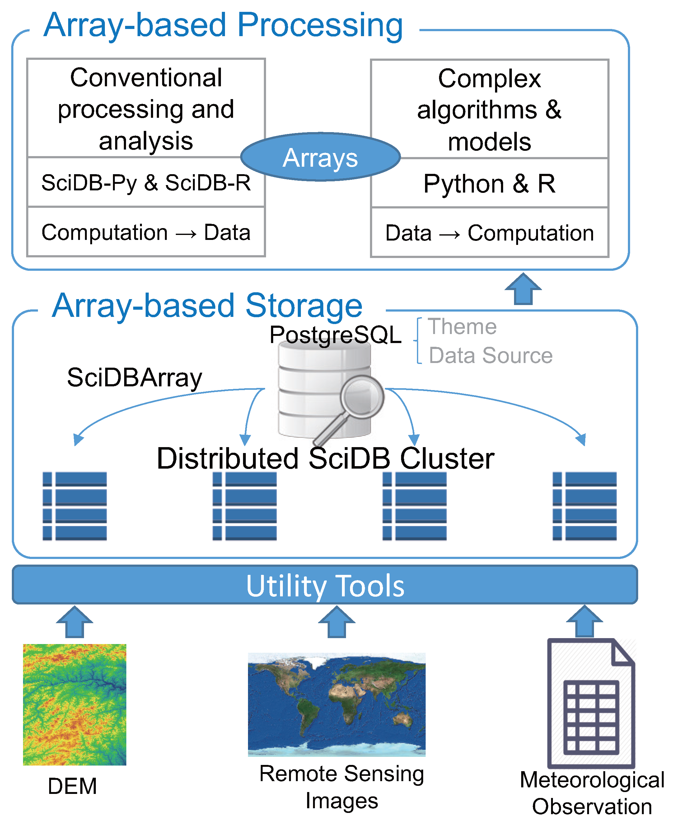
2.2. Method
3. Implementation and Evaluation
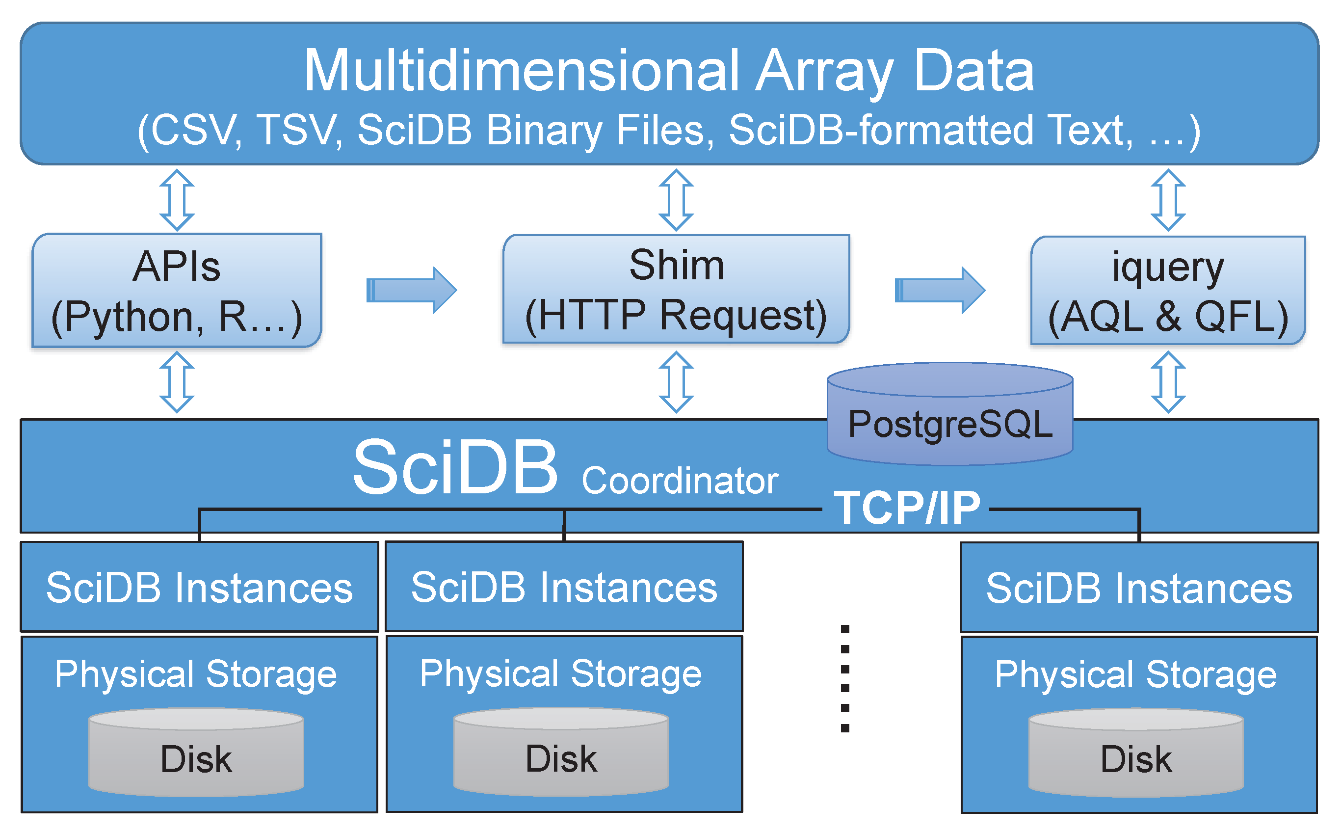
3.1. Implementation
3.2. Comparison with Related Software Solutions for EO Data Cubes
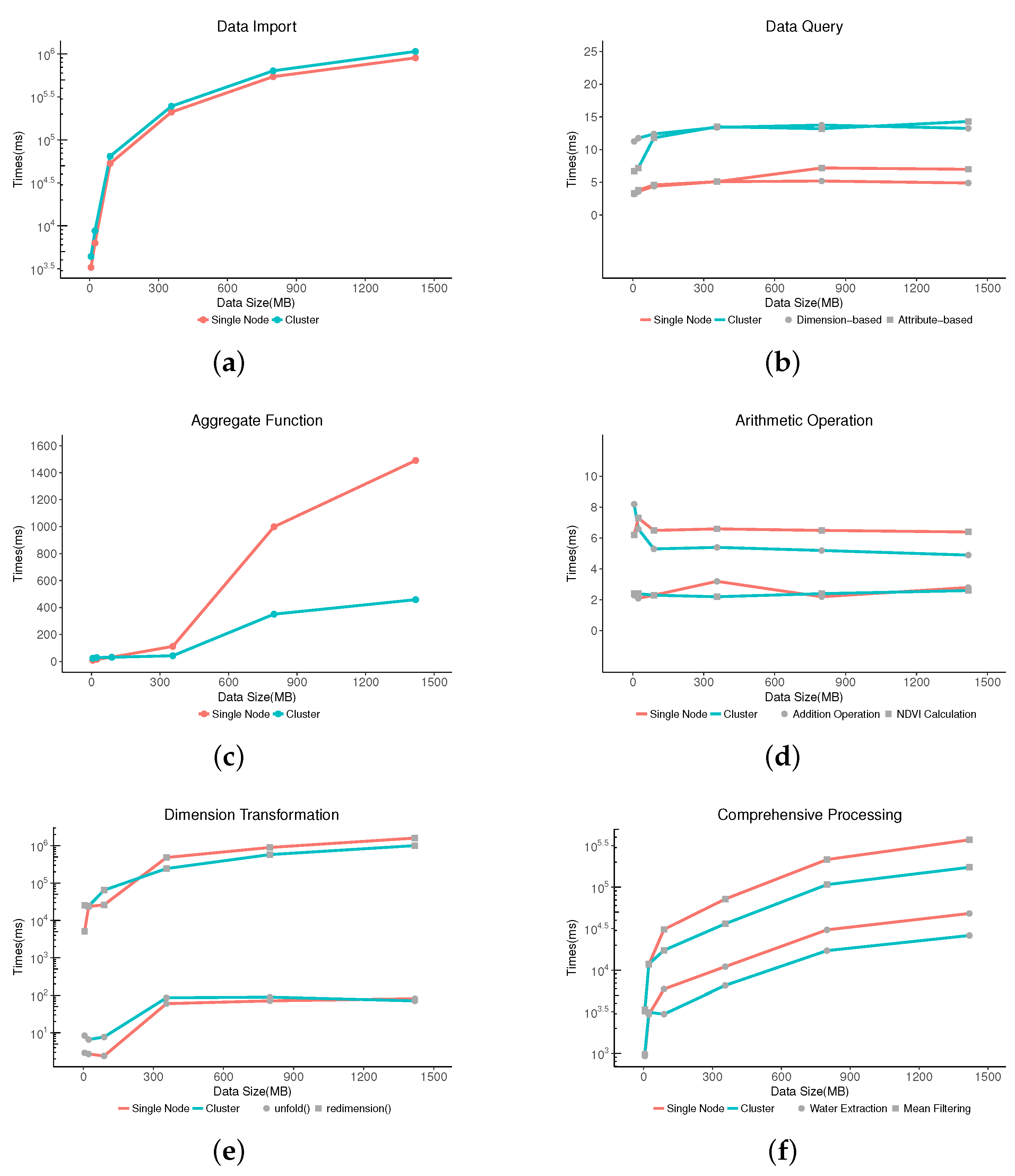
3.3. Performance Evaluation
4. Case Study
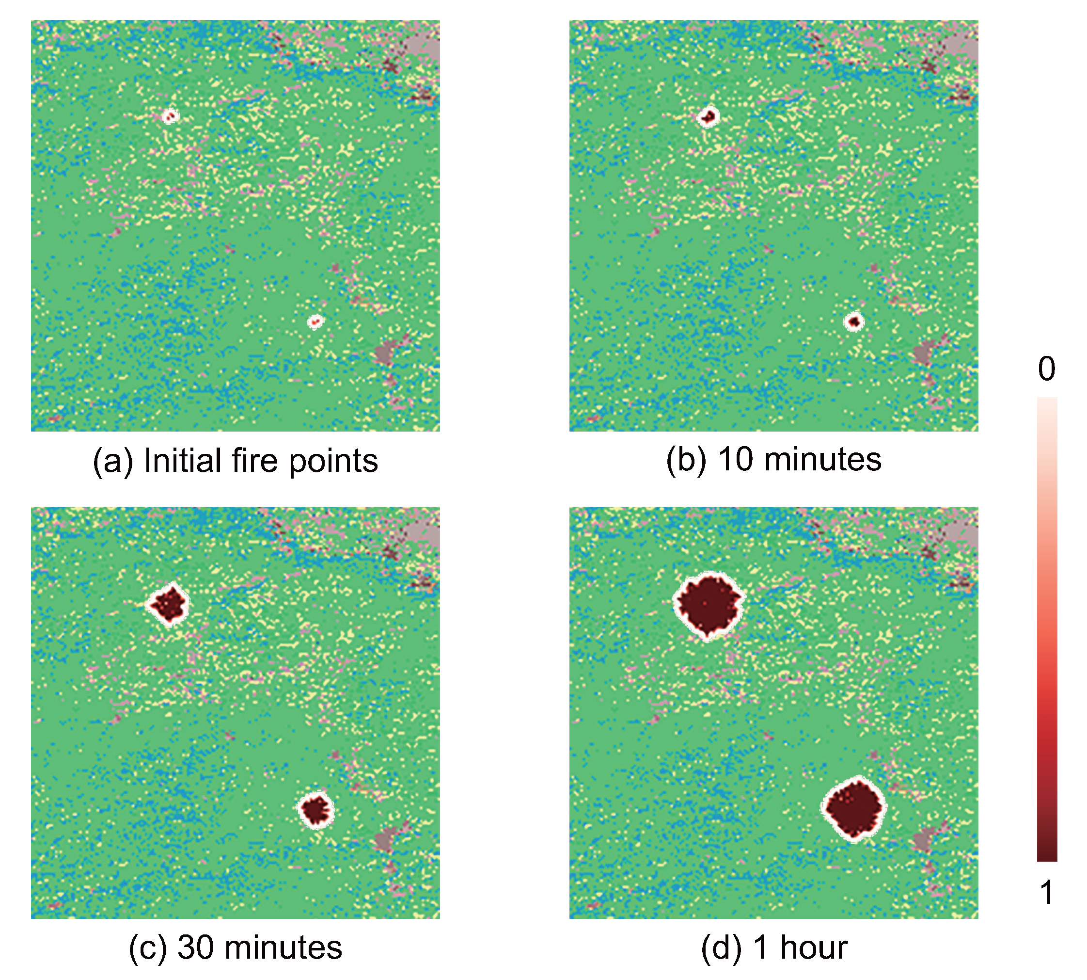
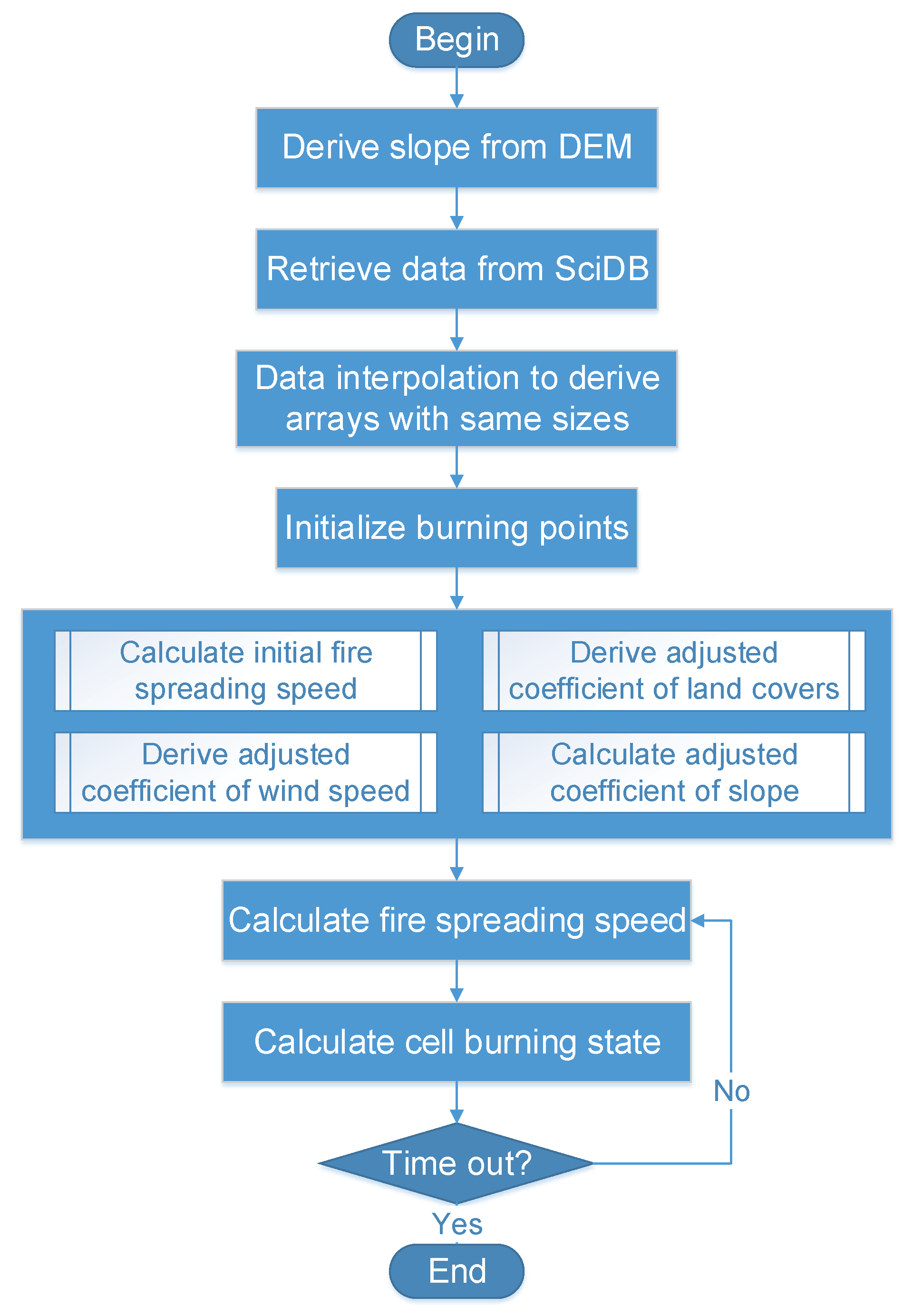
4.1. Forest Fire Simulation Model
4.2. Data Storage Model
4.3. Simulation Walk Through
4.4. Result Analysis
5. Conclusions and Future Work
Acknowledgments
Author Contributions
Conflicts of Interest
References
- Guo, H.; Liu, Z.; Jiang, H.; Wang, C.; Liu, J.; Liang, D. Big earth data: A new challenge and opportunity for Digital Earth’s development. Int. J. Digit. Earth 2017, 10, 1–12. [Google Scholar] [CrossRef]
- Di, L.; Moe, K.; van Zyl, T.L. Earth observation sensor web: An overview. IEEE J. Sel. Top. Appl. Earth Obs. Remote Sens. 2010, 3, 415–417. [Google Scholar] [CrossRef]
- Karantzalos, K.; Bliziotis, D.; Karmas, A. A scalable geospatial web service for near real-time, high-resolution land cover mapping. IEEE J. Sel. Top. Appl. Earth Obs. Remote Sens. 2015, 8, 4665–4674. [Google Scholar] [CrossRef]
- Ma, Y.; Wu, H.; Wang, L.; Huang, B.; Ranjan, R.; Zomaya, A.; Jie, W. Remote sensing big data computing: Challenges and opportunities. Future Gener. Comput. Syst. 2015, 51, 47–60. [Google Scholar] [CrossRef]
- Lee, J.G.; Kang, M. Geospatial big data: Challenges and opportunities. Big Data Res. 2015, 2, 74–81. [Google Scholar] [CrossRef]
- Yue, P.; Ramachandran, R.; Baumann, P.; Khalsa, S.J.S.; Deng, M.; Jiang, L. Recent activities in earth data science. IEEE Geosci. Remote Sens. Mag. 2016, 4, 84–89. [Google Scholar] [CrossRef]
- Yue, P.; Baumann, P.; Bugbee, K.; Jiang, L. Towards intelligent GIServices. Earth Sci. Inform. 2015, 8, 463–481. [Google Scholar] [CrossRef]
- Tan, Z.; Yue, P. A comparative analysis to the array database technology and its use in flexible VCI derivation. In Proceedings of the 2016 Fifth International Conference on Agro-Geoinformatics (Agro-Geoinformatics), Tianjin, China, 18–20 July 2016; pp. 1–5. [Google Scholar]
- Baumann, P.; Dehmel, A.; Furtado, P.; Ritsch, R.; Widmann, N. The multidimensional database system rasDaMan. In Proceedings of the 1998 ACM SIGMOD International Conference on Management of Data (SIGMOD ’98), Seattle, WA, USA, 1–4 June 1998; pp. 575–577. [Google Scholar]
- Brown, P.G. Overview of sciDB: Large scale array storage, processing and analysis. In Proceedings of the 2010 ACM SIGMOD International Conference on Management of Data (SIGMOD ’10), Indianapolis, IN, USA, 6–10 June 2010; pp. 963–968. [Google Scholar]
- Planthaber, G.; Stonebraker, M.; Frew, J. EarthDB: Scalable analysis of MODIS data using SciDB. In Proceedings of the 1st ACM SIGSPATIAL International Workshop on Analytics for Big Geospatial Data. ACM (BigSpatial ’12), Redondo Beach, CA, USA, 6 November 2012; pp. 11–19. [Google Scholar]
- Baumann, P.; Mazzetti, P.; Ungar, J.; Barbera, R.; Barboni, D.; Beccati, A.; Bigagli, L.; Boldrini, E.; Bruno, R.; Calanducci, A.; et al. Big data analytics for earth sciences: The earth server approach. Int. J. Digit. Earth 2016, 9, 3–29. [Google Scholar] [CrossRef]
- Lewis, A.; Oliver, S.; Lymburner, L.; Evans, B.; Wyborn, L.; Mueller, N.; Raevksi, G.; Hooke, J.; Woodcock, R.; Sixsmith, J.; et al. The Australian geoscience data cube—Foundations and lessons learned. Remote Sens. Environ. 2017. [Google Scholar] [CrossRef]
- Baumann, P.; Holsten, S. A comparative analysis of array models for databases. In Proceedings of the International Conferences on Database Theory and Application, Bio-Science and Bio-Technology, DTA/BSBT 2010, Jeju Island, Korea, 13–15 December 2010. [Google Scholar]
- Paradigm4. The Architecture and Motivation for SciDB Paper Is Out; Technical Report; Paradigm4: Waltham, MA, USA, 2016. [Google Scholar]
- Han, J.; E, H.; Le, G.; Du, J. Survey on NoSQL database. In Proceedings of the 2011 6th International Conference on Pervasive Computing and Applications, Port Elizabeth, South Africa, 26–28 October 2011; pp. 363–366. [Google Scholar]
- Harrison, G. Next Generation Databases: NoSQLand Big Data; Apress: New York, NY, USA, 2015. [Google Scholar]
- Yue, P.; Zhang, C.; Zhang, M.; Zhai, X.; Jiang, L. An SDI approach for big data analytics: The case on sensor web event detection and geoprocessing workflow. IEEE J. Sel. Top. Appl. Earth Obs. Remote Sens. 2015, 8, 4720–4728. [Google Scholar] [CrossRef]
- Xiao, Z.; Liu, Y. Remote sensing image database based on NOSQL database. In Proceedings of the 2011 19th International Conference on Geoinformatics, Shanghai, China, 24–26 June 2011; pp. 1–5. [Google Scholar]
- Liu, Y.; Chen, B.; He, W.; Fang, Y. Massive image data management using HBase and MapReduce. In Proceedings of the 2013 21st International Conference on Geoinformatics, Kaifeng, China, 20–22 June 2013; pp. 1–5. [Google Scholar]
- Wang, W.; Hu, Q. The method of cloudizing storing unstructured LiDAR point cloud data by MongoDB. In Proceedings of the 2014 22nd International Conference on Geoinformatics, Kaohsiung, Taiwan, 25–27 June 2014; pp. 1–5. [Google Scholar]
- Appel, M.; Lahn, F.; Pebesma, E.; Buytaert, W.; Moulds, S. Scalable earth-observation analytics for geoscientists: Spacetime extensions to the array database SciDB. In Proceedings of the EGU General Assembly Conference, Vienna, Austria, 17–22 April 2016; Volume 18, p. 11780. [Google Scholar]
- Cudre-Mauroux, P.; Kimura, H.; Lim, K.T.; Rogers, J.; Simakov, R.; Soroush, E.; Velikhov, P.; Wang, D.L.; Balazinska, M.; Becla, J.; et al. A demonstration of SciDB: A science-oriented DBMS. Proc. VLDB Endow. 2009, 2, 1534–1537. [Google Scholar] [CrossRef]
- Brown, P. A survey of scientific applications using SciDB. In Proceedings of the New England Database Day 2015, Cambridge, MA, USA, 30 January 2015. [Google Scholar]
- Warmerdam, F. The geospatial data abstraction library. In Open Source Approaches in Spatial Data Handling; Springer: Berlin/Heidelberg, Germany, 2008; pp. 87–104. [Google Scholar]
- Stonebraker, M.; Brown, P.; Zhang, D.; Becla, J. SciDB: A database management system for applications with complex analytics. Comput. Sci. Eng. 2013, 15, 54–62. [Google Scholar] [CrossRef]
- Aiordăchioaie, A.; Baumann, P. PetaScope: An open-source implementation of the OGC WCS Geo service standards suite. In Proceedings of the Scientific and Statistical Database Management: 22nd International Conference, SSDBM 2010, Heidelberg, Germany, 30 June–2 July 2010; Gertz, M., Ludäscher, B., Eds.; Springer: Berlin/Heidelberg, Germany, 2010; pp. 160–168. [Google Scholar]
- Baumann, P.; Campalani, P.; Yu, J.; Misev, D. Finding my CRS: A systematic way of identifying CRSs. In Proceedings of the 20th International Conference on Advances in Geographic Information Systems (SIGSPATIAL ’12), Redondo Beach, CA, USA, 6–9 November 2012; pp. 71–78. [Google Scholar]
- Rasdaman GmbH. Petascope User Guide. Available online: http://www.rasdaman.org/wiki/PetascopeUserGuide (accessed on 28 June 2017).
- Lewis, A.; Lymburner, L.; Purss, M.B.J.; Brooke, B.; Evans, B.; Ip, A.; Dekker, A.G.; Irons, J.R.; Minchin, S.; Mueller, N.; et al. Rapid, high-resolution detection of environmental change over continental scales from satellite data—The Earth Observation Data Cube. Int. J. Digit. Earth 2016, 9, 106–111. [Google Scholar] [CrossRef]
- Obe, R.O.; Hsu, L.S. PostGIS in Action, 2nd ed.; Manning Publications Co.: Greenwich, CT, USA, 2015. [Google Scholar]
- Wang, Z. Current forest fire danger rating system. J. Nat. Disasters 1992, 3, 39–44. [Google Scholar]
- Mao, X. The influence of wind and relief on the speed of the forest fire spreanding. Q. J. Appl. Meteorol. 1993, 1, 014. [Google Scholar]
- Wolfram, S. Universality and complexity in cellular automata. Physica D 1984, 10, 1–35. [Google Scholar] [CrossRef]
- Paradigm4 Inc. SciDB Reference Guide. Available online: https://paradigm4.atlassian.net/wiki/display/ESD/SciDB+Database+Arrays (accessed on 10 May 2017).
- De Smith, M.J.; Goodchild, M.F.; Longley, P.A. Geospatial Analysis; Troubador Publishing: Leicester, UK, 2009. [Google Scholar]
- Yue, P.; Zhang, M.; Tan, Z. A geoprocessing workflow system for environmental monitoring and integrated modelling. Environ. Model. Softw. 2015, 69, 128–140. [Google Scholar] [CrossRef]


| Earth Observation Data | |||
|---|---|---|---|
| Category | Continuous | Discrete | |
| Data structure | Multidimensional spatiotemporal arrays | ||
| Dimensions: Attributes: (observed values…) | Dimensions: Attributes: (observed values…) | Dimensions: Attributes: (lat, long, observed values…) | |
| Mapping strategy | Six-parameter affine transformation | Scale up the attitude and longitude values by multiplying by ten | / |
| Spatial dimension denotation | 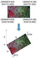 |  |  |
| SciDB | Rasdaman | AGDC | |
|---|---|---|---|
| Implementation | Database plugin | Web application | From scratch |
| Key technologies | SciDB database | Rasdaman database | HPC+HPD (NetCDF) |
| Array database supported | Yes | Yes | No |
| Metadata storage | PostgreSQL (themes, data sources, customized tables) | PostgreSQL (fixed schema, GMLCOV model) | PostgreSQL (fixed schema, JSONB) |
| Coordinate mapping | Affine transformation | GMLCOV model | / |
| Array-based interface provided | Yes | Yes | Yes |
| User interaction | AFL, AQL, C++/Python/R API | WCS & WCPS, rasql, C++/Java/R/ JavaScript API | Python API |
| Processing pattern | In-database | In-database | HPC |
| Advantages | Extensible | Standard | Comprehensive |
| Item | Single Node | Cluster |
|---|---|---|
| Hardware | One server node | Two server nodes |
| Every node shares the same hardware configurations OS: Ubuntu 14.04 x64 CPU: Intel(R) Xeon(R) CPU E5-2692 v2 @ 2.20 GHz, 12 cores RAM: 31.00 GB | ||
| Software | SciDB Community Edition 15.12 PostgreSQL 9.3.16 + PostGIS 2.1.2 | |
| Data | Six remote sensing images: | |
| 5.6 MB (Size: 975 × 993 × 3) | 23 MB (Size: 1950 × 1987 × 3) | |
| 89 MB (Size: 3900 × 3975× 3) | 356 MB (Size: 7801 × 7951 × 3) | |
| 799 MB (Size: 11701 × 11926 × 3) | 1419 MB (Size: 15602 × 15902 × 3) | |
| Item | Description | Example | SciDB Functions |
|---|---|---|---|
| Data import | Load raw data into database | ||
| Typical queries | Queries based on dimension | Retrieve data according to a specific geographic extent | between() |
| Queries based on attribute | Retrieve data where its cell values lie within a given range | filter() | |
| In-database processing | Aggregation operation | Calculate the sum of an array | aggregate(), sum() |
| Arithmetic operation | Add cell values of one array to other array | ||
| Dimension transformation | Change the band of an image as other dimension | redimension(), unfold() | |
| Comprehensive processing | Water extraction | apply(), | |
| Mean filtering | window(), agv() |
| Data Source | Product Name | Fire Growth Factor | Data Size |
|---|---|---|---|
| MODIS | Land Cover Dynamics Yearly L3 Global 1 km | Land cover | 273.7 MB |
| MODIS + MERRA | Land Surface Temperature /Emissivity Daily L3 Global 1 km MERRA-2 () | Surface temperature | MODIS: 13.5 MB MERRA: 397 MB |
| MERRA | MERRA-2 () | Wind speed | 61.3 MB |
| SRTM | SRTM Non-Void Filled, 90 m | Topographic slope | 117.4 MB |
Array for MODIS Land Cover: MCD12Q1_A2013001_h25v03_051<Land_Cover_Type_1 : uint8 , Land_Cover_Type_2 : uint8 , Land_Cover_Type_3 : uint8 , Land_Cover_Type_4 : uint8 , Land_Cover_Type_5 : uint8 > [ y=0:2399,4096,0, x =0:2399,4096,0 , t=0:* ,0,0] Array for MERRA2: MERRA2_400_inst1_2d_lfo_Nx_20131201<PS: float ,QLML: float ,SPEEDLML, float , TLML : float >[y=0:360,2048,0, x=0:575,2048,0,t=0:23,0,0] Array for SRTM DEM: srtm_61_02 <val : int 16 > [y=0:5999,2048,0 ,x =0:5999,2048,0] |
© 2017 by the authors. Licensee MDPI, Basel, Switzerland. This article is an open access article distributed under the terms and conditions of the Creative Commons Attribution (CC BY) license (http://creativecommons.org/licenses/by/4.0/).
Share and Cite
Tan, Z.; Yue, P.; Gong, J. An Array Database Approach for Earth Observation Data Management and Processing. ISPRS Int. J. Geo-Inf. 2017, 6, 220. https://doi.org/10.3390/ijgi6070220
Tan Z, Yue P, Gong J. An Array Database Approach for Earth Observation Data Management and Processing. ISPRS International Journal of Geo-Information. 2017; 6(7):220. https://doi.org/10.3390/ijgi6070220
Chicago/Turabian StyleTan, Zhenyu, Peng Yue, and Jianya Gong. 2017. "An Array Database Approach for Earth Observation Data Management and Processing" ISPRS International Journal of Geo-Information 6, no. 7: 220. https://doi.org/10.3390/ijgi6070220
APA StyleTan, Z., Yue, P., & Gong, J. (2017). An Array Database Approach for Earth Observation Data Management and Processing. ISPRS International Journal of Geo-Information, 6(7), 220. https://doi.org/10.3390/ijgi6070220