Abstract
Assessing model performance is a continuous challenge for modelers of land use change. Comparing land use models with two neutral models, including the random constraint match model (RCM) and growing cluster model (GrC) that consider the initial land use patterns using a variety of evaluation metrics, provides a new way to evaluate the accuracy of land use models. However, using only two neutral models is not robust enough for reference maps. A modified neutral model that combines a density-based point pattern analysis and a null neutral model algorithm is introduced. In this case, the modified neutral model generates twenty different spatial pattern results using a random algorithm and mid-point displacement algorithm, respectively. The random algorithm-based modified neutral model (Random_MNM) results decrease regularly with the fragmentation degree from 0 to 1, while the mid-point displacement algorithm-based modified neutral model (MPD_MNM) results decrease in a fluctuating manner with the fragmentation degree. Using the modified neutral model results as benchmarks, a new proposed land use model, the Dynamics of Land System (DLS) model, for Jilin Province of China from 2003 to 2013 is assessed using the Kappa statistic and Kappain-out statistic for simulation accuracy. The results show that the DLS model output presents higher Kappa and Kappain-out values than all the twenty neutral model results. The map comparison results indicate that the DLS model could simulate land use change more accurately compared to the Random_MNM and MPD_MNM. However, the amount and spatial allocation of land transitions for the DLS model are lower than the actual land use change. Improving the accuracy of the land use transition allocations in the DLS model requires further investigation.
1. Introduction
Land use change is one of the core fields of global environmental change and sustainable development research [1,2]. It is affected by the interaction between natural and human factors. Land use change not only affects the natural basis of human survival and development, but also has an impact on the structural, functional, and ecological characteristics of terrestrial ecosystems [3,4,5,6].
Predicting how land use will change is not only of scientific interest in understanding driving mechanisms of land use change, but is also important for policy making and resource management [1,7]. Therefore, a suite of models has been developed for this purpose [8,9,10,11,12,13]. Based on the different complexities and structures, the models can be divided into statistical models, agent-based models, and integrated models, etc. [14]. Simpler models capture the key characteristics of land dynamics empirically and require less data. They are easily applied but lack the interaction and feedback of geomorphological and ecological processes. Complicated models focus more attention on the interaction and feedback of natural and economic mechanisms, but generally require more data and are difficult to implement.
The Dynamics Land System Simulation (DLS) model is a land use change model that simulates and predicts land use dynamics [15]. The model accounts for the interactions among natural, ecological, socio-economic, and other related processes. By designing different future land use change scenarios, it supports policy making in land use planning, environmental protection, and natural resource management. Different from those conventional models which are limited to the simulation of only one or several land use types [16], the DLS model comprehensively simulates the spatiotemporal pattern of all kinds of land use types at the regional scale. It has solved the problem of discriminating between endogenous and exogenous driving factors of land use changes. In addition, the DLS model quantitatively analyzes the effects of different driving factors by building a spatially-explicit statistical model of the distribution of land use types and driving factors at the pixel level, and it sees the pattern changes in land uses as a dynamic spatiotemporal process. It has improved the scientific and rational nature of predicted and estimated results. This model has been used in some cases [17,18,19], but has rarely been explicitly evaluated for its accuracy of land use change simulation before it is applied. One explicit evaluation was performed by Jiang (2012) in four typical areas in China [19]. The results were compared with the “observed” land use map from the Landsat TM/ETM image using the Kappa statistic and showed good performances. As a new proposed land use change model, comprehensive validation is conducive to future applications of the DLS model.
The assessment of land use change models generally requires the comparison of a simulated land use change map and an actual land use change map over the same time interval [20,21,22]. One method for this assessment is the Kappa statistic [23,24,25]. However, some authors have argued that there are limitations to the end-state assessment of the land use model [26,27,28]. It is not difficult for a land use model to achieve a “very good performance” if the model only changes a small portion of the entire initial map. However, this good agreement does not necessarily indicate an accurate change model. Some studies have made attempts to overcome these shortcomings. Several authors have used the original land use map named the no-change model as a benchmark for comparison to the model results [29]. The “figure of merit” was introduced by Pontius and assesses the agreement of land use changes rather than just the land uses [30].
Except for the pattern validation above, Brown et al. (2013) argue that structural validation that focuses on the match between the processes in the model and the processes operating in the real world also requires development and adoption in the practice of model application [31]. Hagen-Zanker and Lajoie (2008) proposed a new methodological framework to evaluate model performance in which the land use model is compared to the neutral models of landscape change using a variety of metrics to determine to what extent the model performance can be attributed to endogenously modeled processes or to exogenous model inputs [32]. In contrast to the traditional neutral models that create a landscape from a blank or randomized initial map [33,34,35,36], the neutral models of landscape change modify an existing initial landscape subject to the same boundary conditions and constraints as the dynamic models and pose an adequate reference level. The author introduced two types of neutral models which consist of the random constraint match model (RCM) and growing cluster model (GrC).
However, as land use change is a complex process, whether the use of only two neutral models as reference maps is comprehensive and whether there are other spatio-structural neutral models other than the RCM and GrC models requires to be determined. To resolve the above questions, a modified neutral model is designed by combining a density-based point pattern analysis and a null neutral model algorithm that also modifies the existing initial map. This model is an extension of the RCM and GrC models.
Comparisons between the land use change model and the modified neutral model will provide comprehensive insights into how processes that are in the land use change model, but are absent from the neutral model, affect the model performance. This modified neural model would give modelers comprehensive benchmarks to say whether the model of primary interest performs better or worse than an easy to understand benchmark that applies to the same data to which the model of primary interest applies. Thus, the researcher can report how the model performs with respect to an easily understood neutral baseline.
This study aims to apply the modified neutral model as benchmarks to evaluate how well the DLS model predicts land use change for the Jilin Province in China from 2003 to 2013. We firstly introduce the principle and framework of the modified neutral model, and present an example of generating a modified neutral model result. Then, the model output of DLS is compared with those from the modified neutral models, accounting for the sustained land from the initial map. Following this, we discuss the error sources of the DLS model and the advantages of the modified neutral model in the model evaluation. Finally, we offer suggestions as to how we should apply DLS to make its predictions more informative and propose future research on the modified neutral model.
2. Data and Methods
2.1. Study Area and Data Source
The study area is Jilin Province, which is located in northeastern China (40°50′–46°19′ N and 121°38′–131°19′ E) (Figure 1). It has an area of 187,400 km2, which is 2% of China’s total area. The eastern area of the province is mountainous and the central and western areas are plains. Crop land, forest land, and grass land cover 84.1% of the province’s total area. The crop and grass land is mainly distributed in the central and western plains and the forest land distributed in the eastern mountainous. Agriculture and forestry are the primary economic activity. This province is not only a major grain production area, but also boasts a rich biodiversity and important ecological functions. Over the last 15 years, this province has undergone some profound changes. The population increased from 27.04 million inhabitants in 2003 to 27.51 million in 2013. The economy has also grown and the urban built-up area has expanded rapidly.
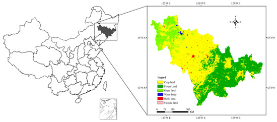
Figure 1.
Study area location map.
The land use model is calibrated over the period 2003–2013. In this period, the increase of forest and built land areas and the reduction of grass and crop land were the main processes of land use change. Crop land was mainly converted into forest land due to the government policies which were designed to achieve the restorative development of forest, control water and soil loss, and protect the ecological environment after the devastating flood in the summer of 1998.
The data required in this study include: land use maps, geophysical data, and socio-economic datasets. The land use maps during 2003–2013 are derived from NASA’s Earth Observing System Data and Information System (EOSDIS). The coverage is a grid with a 500 m cell size. We maintain the original resolution to avoid errors related to resampling and reclassified the map into six kinds of land-use categories: crop land, forest land, grass land, water body, built land, and unused land.
The geophysical data required include information on the terrain slope, information on soil property variability, measurements on climatic change, and the Normalized Difference Vegetation Index (NDVI) remote sensing data. Information on the terrain slope is derived from DEM data according to surface analysis, and is resampled into the 500 m × 500 m grid cell data. The meteorological data, consisting of the annual temperature and annual precipitation, are acquired from meteorological station observation records. Information on the soil property comes from the second national soil survey of China. These sampling data are interpolated into the 500 m × 500 m grid cell data according to the Kriging algorithm. NDVI data are extracted from the MODIS product MOD13Q1 with a 500 m cell size.
The socio-economic dataset consists of variables such as the population density, Gross Domestic Product (GDP), agricultural production, agricultural population proportion, timber production, gross output value of forestry production, and binary values, e.g., if it is a natural reserve. These continuous data are derived from provincial statistics and are linked with city level spatial units to understand spatialization. The policy variables include the Logging Ban Project and the involvement of the Grain for Green Project which have been released at the national level. These policies are designed to protect the ecological environment and were implemented in 1998 and 1999, respectively.
2.2. Modified Neutral Models
The RCM and GrC models are conservative by minimizing change [31]. The RCM approach chooses a random location of one randomly-chosen, decreasing land class, and then converts it to one randomly-chosen, increasing land class, until the net changes of all land classes have been made. The GrC simulates the locations of changes randomly along the edges of existing pairs of randomly-selected, decreasing and increasing land classes; the decreasing land class is converted to the increasing land class.
In this study, we set the fragmentation degrees of the RCM and GrC models to 0 and 1, respectively. In addition, the fragmentation degree correlates with the point density. Because the number of changed cells is known, the fragmentation degree is directly related to the distribution area of the changed cells. In the RCM model, the distribution areas contain all the patches of the overrepresented class in the initial map. The distribution areas in the GrC model are the cells of the overrepresented class that are close to the underrepresented class patches.
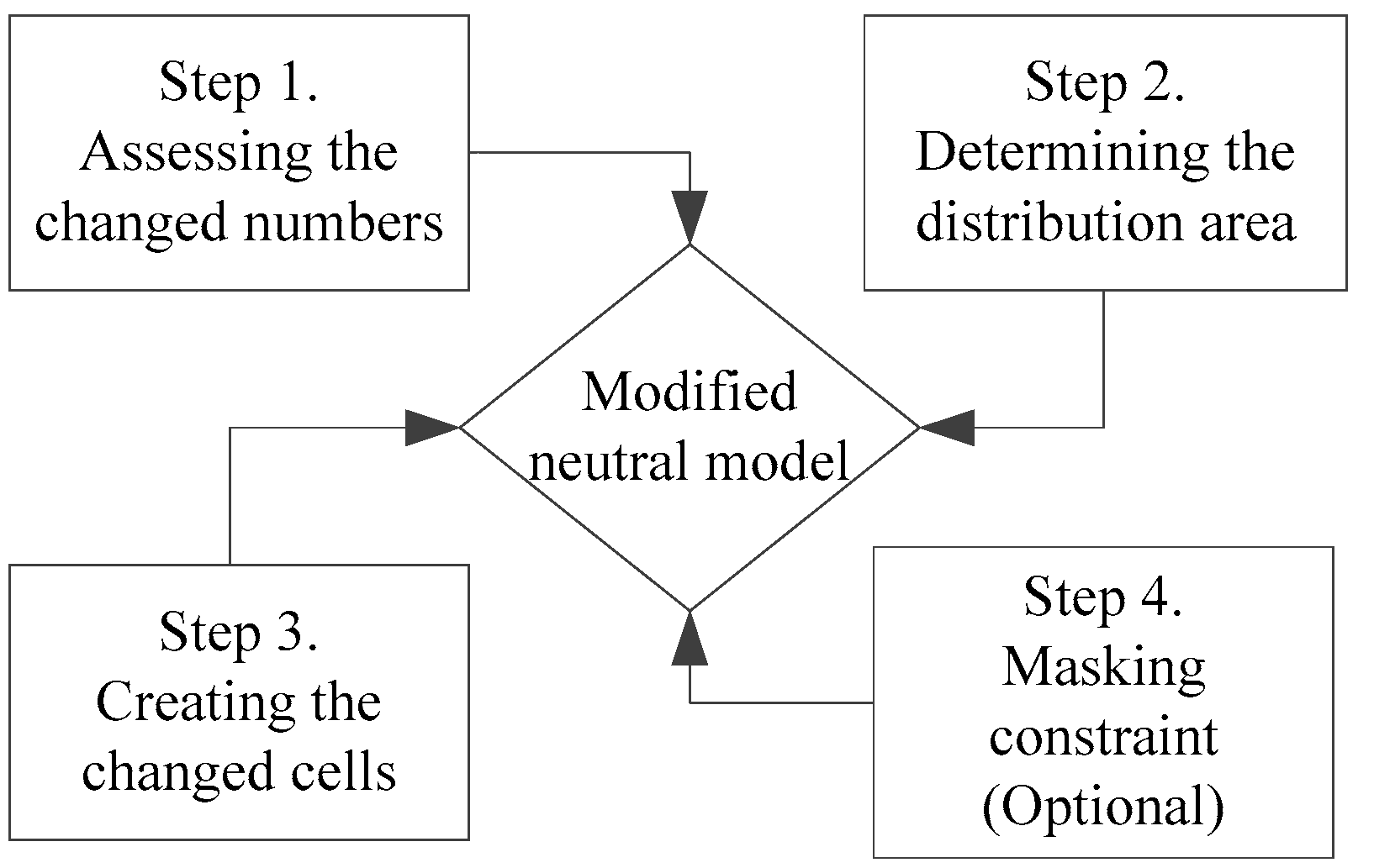
Based on the above settings and analysis, a modified neutral model is designed to produce more generalized results compared to the RCM and GrC models for any fragmentation degree between 0 and 1. This model transforms the fragmentation degree setting to the point density setting or the distribution area setting and uses the null neutral model algorithm to create the changed cells. As the fragmentation degree decreases, the point density decreases and its distribution area close to the underrepresented class increases, resulting in more fragmented patterns. The modified neutral model is also subject to the same boundary condition and constraints as the evaluated model. It follows the notion of changing as little as possible [32,37]. In this paper, the modified neutral model simulates the same amount of changed cells as the DLS model, and the difference from DLS is the spatial allocation of the changing cells. Therefore, the modified neutral model poses an adequate reference level. The flowchart of generating the modified neutral model results is shown in Figure 2. The data used in this model must be in raster format (grid-based data).

Figure 2.
Flowchart for generating a modified neutral model result.
- Step 1: Assessing the number of changed cells.First, count the cells for all of the classes in the initial map and the final map. As one class may transform to two or more classes, based on the degree of transfer difficulty between the land use classes, we should determine the transfer probability between the different classes. Based on the probability, determine the number Nij of class i cells in the initial map that transform to class j.
- Step 2: Determining the distribution area of the changed cells.This step includes two sections. First, calculate the number of cells (Mj) that compose the distribution area using the following equation:where Nij is the number of class i cells in the initial map that transform to class j. p is the parameter that controls the degree of cell fragmentation and ranges from 0 to 1. Mi is the number of class i cells in the initial map.Mj = (Mi − Nij) × p + NijSecond, calculate the shortest distance between each cell in land class i and the patches of land class j using the neighborhood analysis tool in ArcMap 10.1 software. Place the shortest distances in ascending order, and select the top Mj cells. These selected cells compose the distribution area.
- Step 3: Creating the changed cells in the distribution area.Null neutral models are useful tools for testing the effect of a particular modeled process on observed patterns, as they create landscape patterns in the absence of those specifically processed from a blank initial map. However, they never account for the initial land use pattern. The generated landscape is not an appropriate reference map. The combination of null neutral modes and distribution area of the changed cells (generated in step 2) overcomes this shortcoming. In the distribution area, the null neutral model algorithm is applied to distribute allocations of the Nij changed cells. The algorithms of the null neutral models could include the simple random algorithm, mid-point displacement algorithm (MPD) [38], random rectangular cluster algorithm [39], modified random clusters algorithm [40], etc.In this case, the random algorithm and mid-point displacement algorithm are used to create the changed cells in the distribution area. The random algorithm is a simple and easily understood null neutral model. There is no spatial autocorrelation as each element in the array is independently assigned a value. It is usually used as a baseline for comparison. The mid-point displacement algorithm is a fractal algorithm in which the level of autocorrelation can be controlled from 0 to 1. It has been widely used in simulating landscape patterns and is integrated into standalone software such as RULE and the subsequent QRULE. When using the random algorithm, the changed cells are a series of randomly distributed cells in the distribution area. The mid-point displacement algorithm can only be applied to square arrays of specific sizes. Therefore, to enable a two dimensional array of any size to be created, we create an array that is larger than the distribution area extent, but is the minimum-sized square that will cover the desired extent, from which a slice of the required dimensions is then extracted. The two kinds of null neutral models are created by a PYTHON package of NLMpy [41]. The fragmentation degree parameter for the null neutral model algorithms is the same as parameter p in Equation (1).
- Step 4: Masking constraint (Optional).In land use models, a mask is sometimes applied to separate the changed and unchanged areas. This enables the land use model result to be subject to the same changing boundary conditions as the actual land use change. The modified neutral model is based on an existing initial land use map that minimizes change, and the masking constraint could also be applied if necessary.
A simple example of generating a modified neutral model result based on the simple random algorithm for p = 0.3 is given below.
Suppose Figure 3a,b are the initial map (T0) and final map (T1), respectively. The light-grey cells are class 1 and the black cells are class 2, and each class consists of 50 cells.
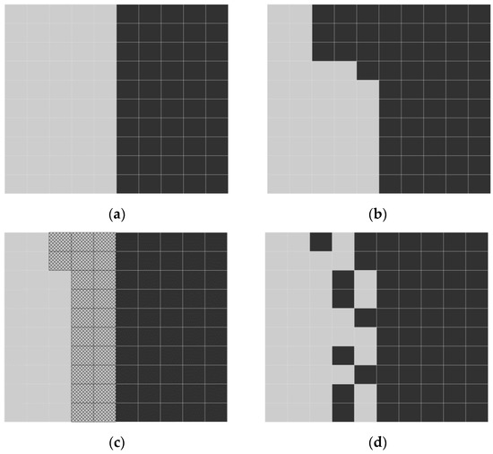
Figure 3.
Generation process of Random_MNM for p = 0.3: (a) Initial map; (b) Finial map; (c) Distribution area; (d) Random_MNM result, p = 0.3.
- Step 1: Assessing the number of changed cells.Class2 increased by 10 cells and class 1 decreased by 10 cells from T0 to T1.
- Step 2: Determining the distribution area.
- (1)
- Calculate the number of cells in the changed area.where 50 is the number of class 1 cells in the initial map, 10 is the number of class 1 cells in the initial map that transform to class 2, 0.3 is the parameter we set that controls the degree of cell fragmentation, and the result M = 22 is the number of cells in class 1 that compose the distribution area.M = (50 − 10) × 0.3 + 10 = 22
- (2)
- According to the shortest distance principle, select 22 cells in class 1 that are close to class 2. The selected cells compose the distribution area which is covered by the net in Figure 3c.
- Step 3: Creating the changed cells.When using the random algorithm, directly create 10 random cells in the distribution area. Then, convert these cells from class 1 to class 2 (Figure 3d). When using the mid-point displacement algorithm, the generation process is complex. First, the NLMPy produces a 10 × 10 array with a fragmentation degree parameter of 0.3 using the mid-point displacement algorithm, in which the elements of the array at each row and column position contain a value from 0 to 1. A 10 × 10 array is the minimum-sized square cover distribution area extent because the extent of netted cells is 10 × 3. Then, extract the required area from the produced patterns using the 22 netted cells as a mask. Following this, the ‘classify array’ function in NLMpy is employed to classify the 22 cells into two parts which consist of 10 cells and 12 cells, respectively. Finally, choose the 10 cells and converted them from class 1 to class 2, through which the changed cells are obtained.As we do not set the unchanged area, Step 4 is not performed. Figure 3d is the modified neutral model result based on the random algorithm for an aggregation of 0.3.
2.3. DLS Model
The DLS model considers the links among related models of nature, ecology, and economy. It also extracts the decision-making reference information used in land use planning, environmental planning, and the management of natural resources by designing different scenarios of a changing regional land use area. Users of the DLS model can input nonlinear demand change, different conversion rules, and driving factors at different pattern changes in land uses to simulate and analyze the complex changes in regional land use patterns. The DLS model also considers the influence of macroscopic factors such as topography, environment, trade, and institutional arrangement and land management policies to more accurately simulate possible scenarios of pattern changes in land uses. The DLS model presumes that land use pattern change is influenced by both historic pattern changes in land uses and driving factors within the pixel and neighboring pixels. Decisions of land use planners have an important influence on the pattern changes in land uses, especially at the regional level.
The DLS model is composed of three modules: the scenario design module, the driving mechanism analysis module, and the spatial allocation module (Figure 4). The scenario design module provides the annual demand of each land use class. The driving mechanism analysis module calculates the spatial statistical relationship between land use distribution and the driving factors, and it analyzes the driving factor’s influence on the land use distribution. The spatial allocation module creates the spatial distribution of land use change based on land supply and demand balance analysis.
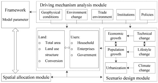
Figure 4.
Principle of the DLS model [15].
DLS is a software tool developed based on the DLS model for the dynamic simulation of land use pattern changes. It can measure the influence of driving factors that are closely associated with changes in the land use pattern, including natural conditions, socioeconomic factors, and even land use management policies. It can simulate the spatial-temporal process of the pattern changes of land uses and export maps of pattern changes of land uses with a high spatial and temporal resolution by setting conversion rules of land use types and designing change scenarios. In this paper, the DLS software is applied to predict the land use map for Jilin Province in 2013, based on the baseline land use map of 2003. As an input parameter, the transition probabilities between different land use classes are shown in Table 1. The driving factors behind land use change are analyzed with the explanatory linear model of land use pattern (ELMLUP) built at the cell level.

Table 1.
Transition probabilities of each land use class.
2.4. Metrics to Evaluate the Model
In this study, two-map and three-map comparisons are applied for the assessment of the DLS model and the modified neutral model. The two-map comparison assesses the agreement between the actual map and the simulated map, and the result is expressed using the Kappa coefficient. Kappa can be divided into Kappahistogram and Kappalocation.
The three-map comparison involves the actual map at the start of the simulation, the actual map at the end of the simulation, and the simulation map at the end of the simulation [34]. It assesses the agreement between the actual class transitions and the simulated class transitions. To compute the expected agreements, we define the Kappain-out coefficients. The calculation steps are as follows: first, determine the actual class transition map from the original map (T0) to the actual map (T1) using land use class transition analysis. Using the same analysis, we obtain the simulated class transition maps from the original map to the model simulated maps. Second, the contingency table between the actual class transition map and simulated class transition map is created using the tabulate area function in ArcMap 10.1 software (Table 2). In contrast to the n×n contingency table for the Kappa statistic, this contingency table is expanded to [n × (n − 1) + 1] × [n × (n − 1) + 1], where n represents the number of land use classes. Finally, based on the obtained contingency table, Kappain-out, Kappain-out-location, and Kappain-out-histogram are calculated using Equations (2)–(4), respectively.
where pii represents cells that have the same value in both transition maps. pin and pni represent the fraction of cells that have value i in two maps. The values for Kappain-out range from 0 to 1, with the same criteria as Kappa.
Table 2.
Contingency table between two transition maps.
3. Results
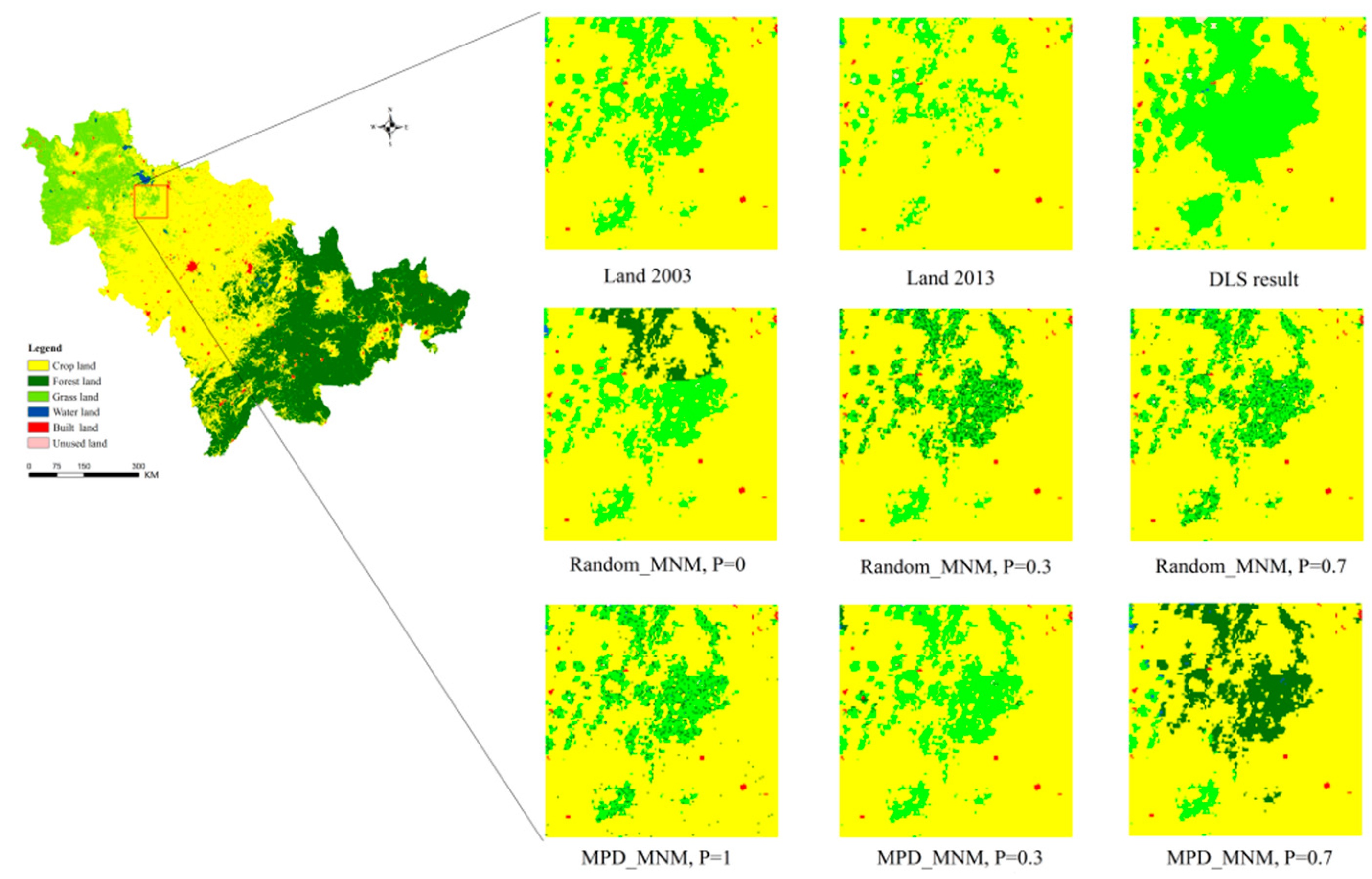
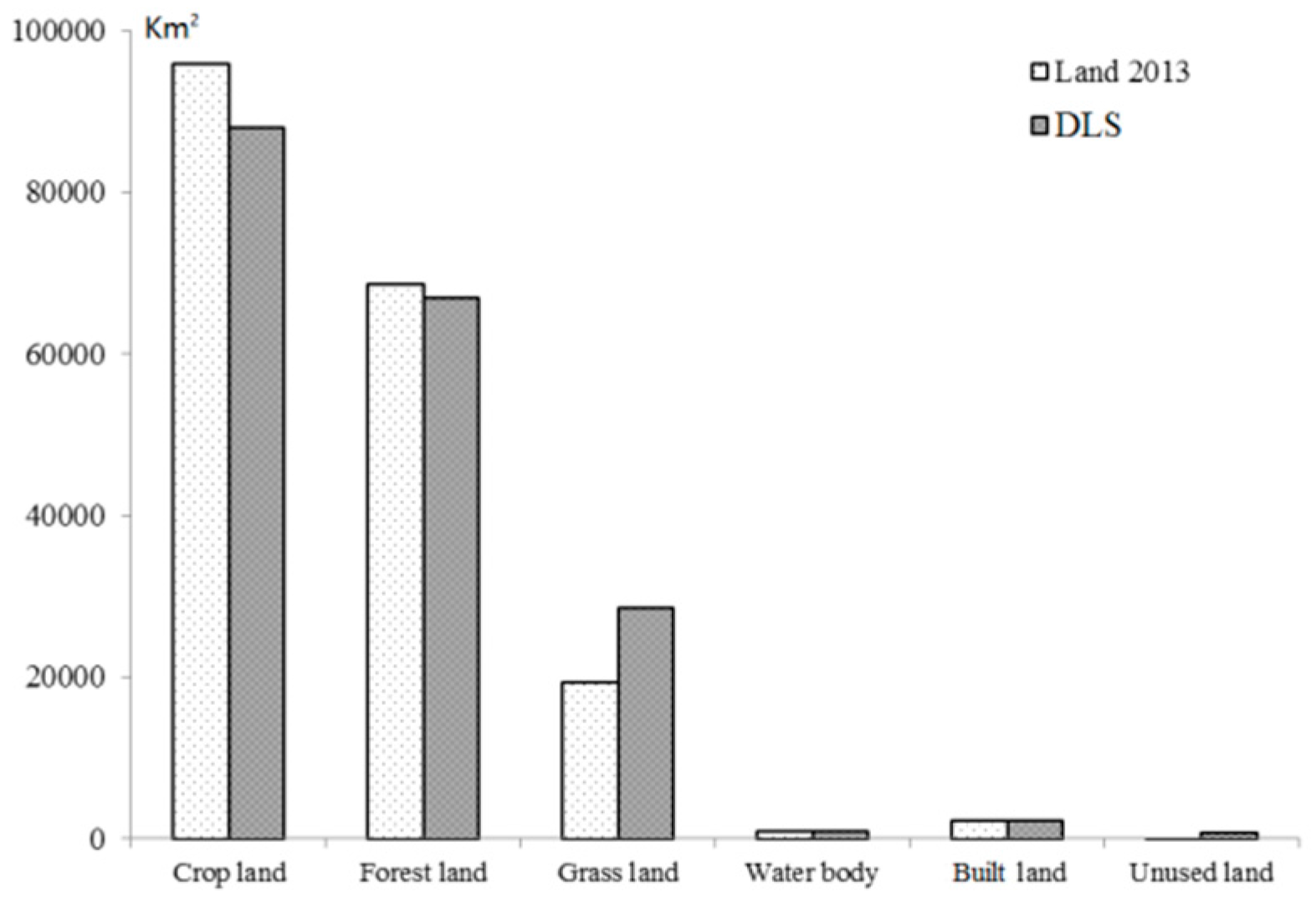
The Jilin land use maps in 2003 and 2013, as well as the simulated maps, are shown in Figure 5. The statistical areas (Figure 6) show that the DLS model achieves a close result to the actual map for forest land, water body, and built land, while the area accuracy of crop land, grass land, and unused land is relatively low.
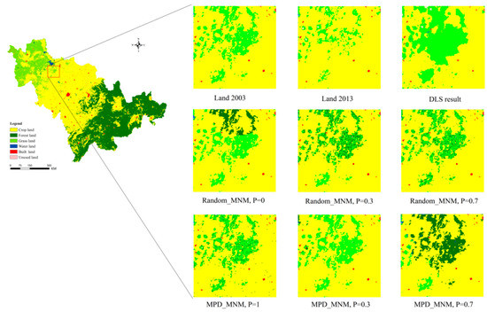
Figure 5.
Sample maps of the simulation results.

Figure 6.
Area statistics of each land use class in the Land 2013 map and the DLS result.
Using the final time land use map (Land 2013 map) as a standard, a map comparison is performed to evaluate the accuracy of the DLS model using two types of metrics. The modified neutral model and the no-change model results are used as benchmarks. The modified neutral model using the random algorithm is named Random_MNM, and that using the mid-point displacement algorithm is named MPD_MNM. Their aggregations are all between 0 and 1 with 0.1 intervals. Because the Random_MNM and MPD_MNM for p = 0 and p = 1 have the same results, the modified neutral model generates 20 neutral model results.
3.1. Kappa Result Comparison
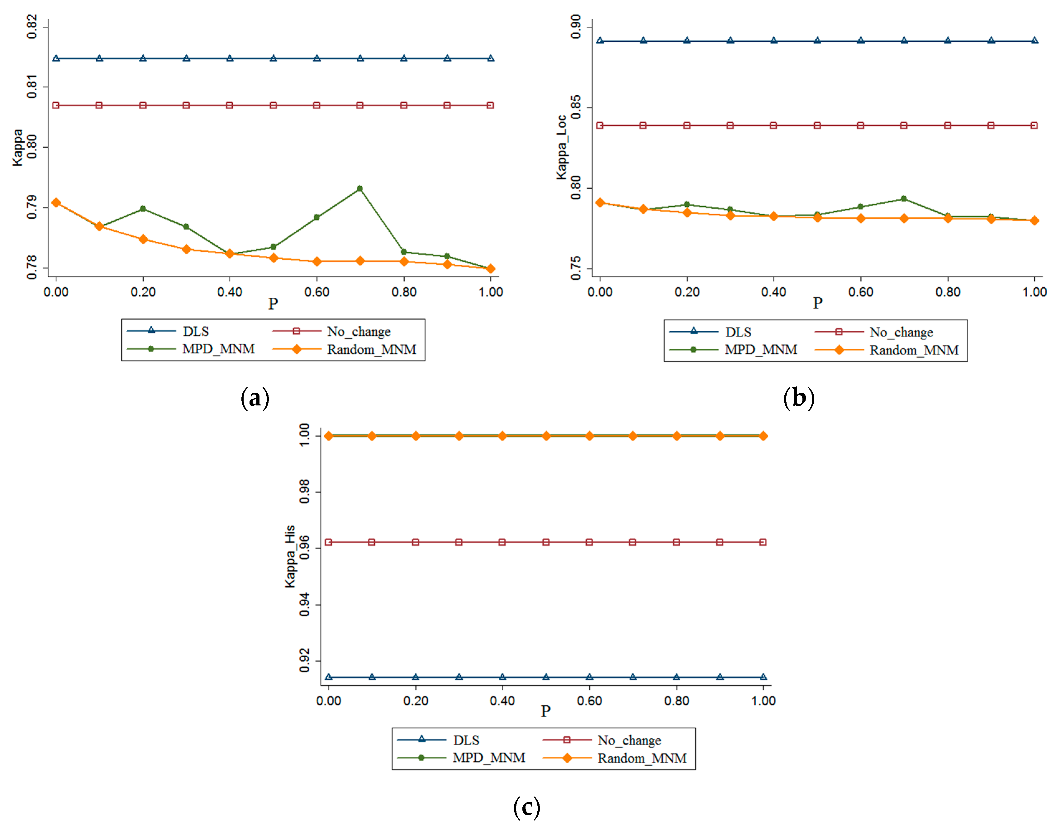
The Kappa series’ scores for the actual map and each simulation map are shown in Figure 7. The Kappa comparison results (Figure 7a) indicate that when implementing different null neutral model algorithms, the change trend of the modified neutral model results with the fragmentation degree from 0 to 1 performs differently. The random algorithm-based modified neutral model (Random_MNM) results decrease regularly with the fragmentation degree from 0 to 1. The maximum and minimum Kappa values are obtained when p = 0 and p = 1, respectively. However, the mid-point displacement algorithm-based modified neutral model (MPD_MNM) results decrease in a fluctuating manner with the fragmentation degree. The minimum Kappa value is obtained when p = 0, but the maximum Kappa value is obtained when p = 0.7. In addition, all the Kappa scores of the neutral model results are higher than 0.78, except for the Random_MNM result for p = 1, indicating that most of the modified neutral models have a good simulation performance based on the Kappa evaluation standard.

Figure 7.
Comparison of the Kappa series’ scores: (a) Kappa scores; (b) Kappalocation scores; (c) Kappahistogram scores.
The DLS model and no-change model perform better than all the modified neutral models, and the DLS model obtained the highest Kappa scores. The Kappa score for the no-change model is 0.807, which represents good agreement. Because the no-change model is the initial map, this indicates that there are a few land use changes occurring over the simulation period.
In terms of the land use change locations (Figure 7b), the DLS model outperforms the neutral models and the no-change model. Additionally, the change tendencies with the Kappa scores are similar. Because the number of changed cells is known in the modified neutral model, the Kappahistogram values of the Random_MNM results and the MPD_MNM results are expected to be higher than those of the DLS and the no-change model results (Figure 7c).
3.2. Kappain-out Result Comparison
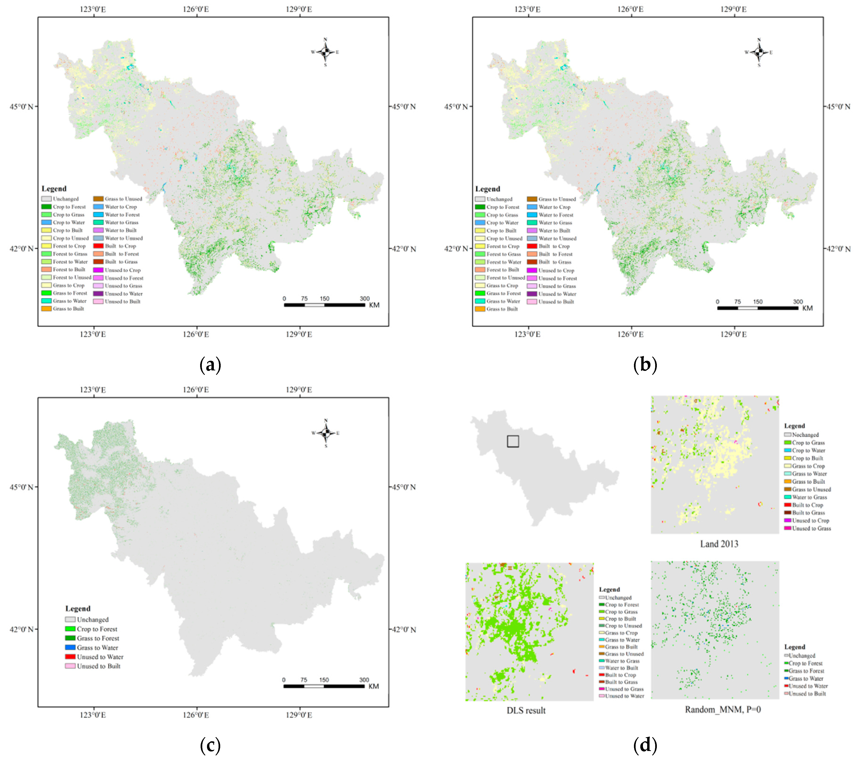
For the land use class transition analysis, we obtain the land use transition maps that start from the initial map of the actual land use map (Land 2013 map), the DLS results, and the modified neutral model results (Figure 8). The transition map of the no-change model is null because it is the same as the initial map. Figure 6 illustrates that the land use transitions of the Land 2013 map and the DLS results are more complex than those of the modified neutral model. This is because the modified neutral model only changes cells in the overrepresented land use classes.
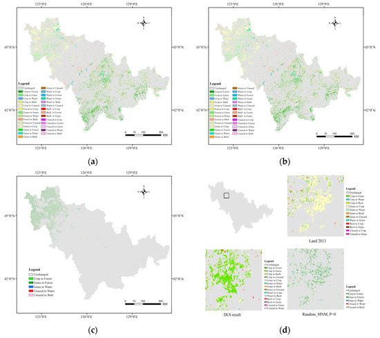
Figure 8.
Land use transition maps: (a) Land 2013 map; (b) DLS result; (c) Modified neutral model, Random_MNM, p = 0 as an example; (d) Sample maps of the transition maps.
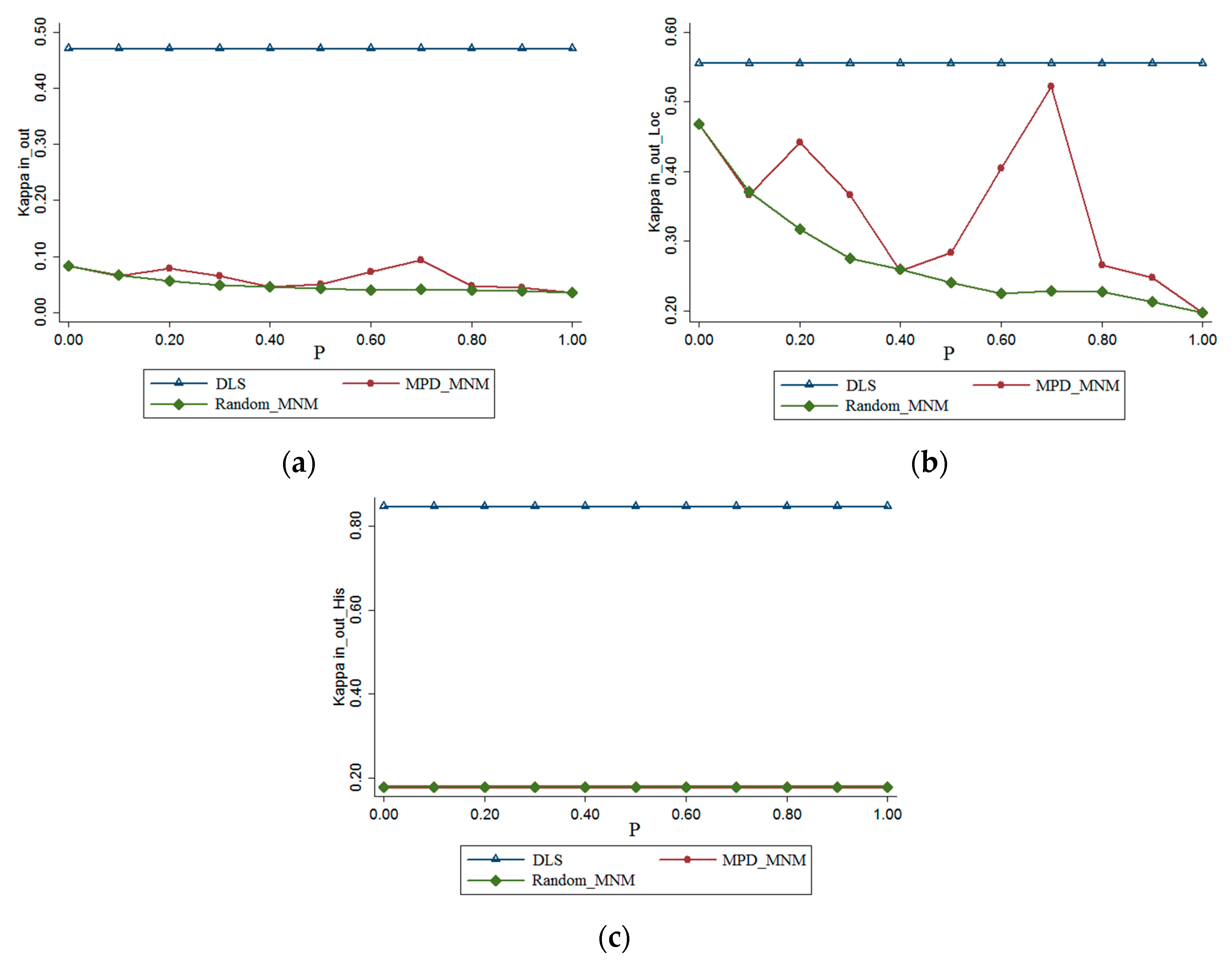
Based on the transition maps, the Kappain-out series’ scores are calculated, and the results are shown in Figure 9. The change trend for the Kappain-out scores of the modified neutral model results is similar to those for the Kappa scores (Figure 9a). However, the relative relationship between the modified neutral model and DLS results for the Kappain-out scores is different. The Kappain-out scores of all the modified neutral model results are less than 0.1, which means that there are fewer of the same class transitions that appear in both the modified neutral model and in reality. The DLS model has the highest score of 0.47, and this indicates that the DLS model has more accurate class transition simulations than the modified neutral model. The results for the transition locations show that the MPD_MNM result for p = 0.7 has the closest score to that of the DLS model (Figure 9b). In terms of the land use transition quantities (Figure 9c), the DLS model outperforms all the modified neutral model results, which is the exact opposite of the Kappahistogram comparison result.

Figure 9.
Comparison of the Kappain-out series’ scores: (a) Kappain-out scores; (b) Kappain-out-location scores; (c) Kappain-out-histogram scores.
4. Discussion and Conclusions
Comparing land use models with RCM and GrC neutral models provides a new method to evaluate land use models, especially for the land use change process. When using the RCM and GrC models, researchers may have a default assumption that RCM and GrC represent the maximum and minimum values (or minimum and maximum values) and that the neutral models change regularly with the fragmentation degree. However, we cannot guarantee that this assumption is correct. Research has rarely focused on the middle fragmentation degrees between the RCM and GrC models. Xiu et al. (2017) [42] used the mid-point displacement algorithm to create landscape spatial patterns starting from a blank initial situation with fragmentation degrees from 0 to 1 and compared them to actual landscapes using landscape metrics. They found that the simulated landscape patterns change irregularly with the fragmentation degree and that they have cross points with the actual landscapes. Therefore, it is essential to obtain more general neutral model results that modify the existing landscape and explore whether they will also change irregularly with the fragmentation degree.
From the modified neutral model, we obtain more generalized neutral model results compared to the RCM and GrC models. The simulated results show that using different null neutral model algorithms in the modified neutral model leads to a different change trend with the fragmentation degree. When using a random algorithm, the results change regularly with the fragmentation degree, and the RCM (equal to an aggregation of 0 in modified neutral model) and GrC (equal to an aggregation of 1 in modified neutral model) models represent the minimum and maximum values of Kappa and Kappain-out scores. However, the use of the mid-point displacement algorithm in the modified neutral model results in fluctuating changes, and the highest value appeared in the middle of the fragmentation degree. The results indicate that the modified neutral model could provide more diverse results than the RCM and GrC models, and it has more advantages in being used as a reference map in map comparisons.
The DLS model is assessed using the modified neutral models as benchmarks with both a two-map and three-map comparison. The comparison results indicate that the DLS model could simulate land use change more accurately than the modified neutral models and the no-change model with higher Kappa and Kappain-out values. The high Kappa score of the no-change model is impressive, even though it does not simulate any changes at all. This indicates the high accuracy simply due to land use persistence, but not for the simulation process of the land use model. Consequently, the Kappa statistic is not an appropriate measure for the land use accuracy assessment. This is also consistent with the findings of other authors [43]. The transition maps show the land use cell transitions in detail. According to the transition maps, the actual land use change is a complex class transition process. The Kappain-out scores based on the transition map performed better than Kappa, which avoids a false impression of accuracy caused by high Kappa scores for the models with only a small amount of change. Due to the lack of a simulation mechanism, modified neutral model results have a poor performance in the class transition simulation. The DLS model performs better than the modified neutral model, but there are still significant differences with the actual land use transition for the amount and the spatial distribution. The simulation uncertainty indicates that there are still some mechanisms which are not considered for the DLS model in this study and that more driving factors need to be considered.
We call for a more appropriate application of the DLS model, including emphasizing the selection of an appropriate mechanism model to predict and analyze the regional land system change, and implementing the high spatial and temporal resolution remote sensing data. The DLS models in this paper are analyzed at a single resolution. However, scale is also an important part of evaluating models, so multi-scale comparison analyses need to be further studied. Although the modified neutral model is more comprehensive than the RCM and GrC models, it generates too many results in this case, which increase the comparison workload. For future research, selecting fewer representative neutral model results as benchmarks is recommended. In addition, except for the Kappa and Kappain-out scores, other kinds of metrics to assess the accuracy of the model could also be employed in future map comparisons, e.g., landscape metrics which assess the land use spatial patterns, and other kinds of three-map comparison metrics including Misses, Hits, Wrong Hits, False Alarms, and Correct Rejections.
Acknowledgments
We are grateful to Wei Wu in the University of Southern Mississippi for her help with neutral models. The paper was supported by the National Statistical Science Research Project (No. 2016LY76), the China Postdoctoral Science Foundation (No. 2015M572061), and the General Program of Shandong Natural Science Foundation (No. ZR2015FM014).
Author Contributions
Yingchang Xiu designed the methodology of research, coordinated the implementation of the proposed approach, and wrote the paper; Wenbao Liu and Wenjing Yang contributed to implementing the approach and preparing the illustrative figures.
Conflicts of Interest
The authors declare that there is no conflict of interests regarding the publication of this article.
References
- Turner, B.L.; Skole, D.L.; Sanderson, S.; Fischer, G.; Fresco, L.O.; Leemans, R. Land-Use and Land-Cover Change: Science/Research Plan; IGBP, 1995 (IGBP Report 35); International Geosphere-Biosphere Programme: Stockholm, Sweden, 1995; p. 132. [Google Scholar]
- Young, B.; Noone, K.; Steffen, W. Science Plan and Implementation Strategy; IGBP Report No. 53/IHDP Report No. 19; IGBP Secretariat, Global Land Project (GLP): Stockholm, Sweden, 2005; p. 64. [Google Scholar]
- Verburg, P.H.; Schot, P.P.; Dijst, M.J.; Veldkamp, A. Land use change modelling: Current practice and research priorities. GeoJournal 2004, 61, 309–324. [Google Scholar] [CrossRef]
- Ghaffarzadegan, N.; Lyneis, J.; Richardson, G.P. How small system dynamics models can help the public policy process. Syst. Dynam. Rev. 2011, 27, 22–44. [Google Scholar] [CrossRef]
- Rounsevell, M.D.A.; Pedroli, B.; Erb, K.H.; Gramberger, M.; Busck, A.G.; Haberl, H.; Kristensen, S.; Kuemmerle, T.; Lavorel, S.; Lindner, M.; et al. Challenges for land system science. Land Use Policy 2012, 29, 899–910. [Google Scholar] [CrossRef]
- Reidsma, P.; König, H.; Feng, S.; Bezlepkina, I.; Nesheim, I.; Bonin, M.; Sghaier, M.; Purushothaman, S.; Sieber, S.; van Ittersum, M.K.; et al. Methods and tools for integrated assessment of land use policies on sustainable development in developing countries. Land Use Policy. 2011, 28, 604–617. [Google Scholar] [CrossRef]
- Veldkamp, T.; Verburg, P.H.; Kok, K.; Koning, F.D.; Soepboer, W. Spatial Explicit Land Use Change Scenarios for Policy Purposes: Some Applications of the CLUE Framework. In Linking People, Place, and Policy; Walsh, S.J., Crews-Meyer, K.A., Eds.; Springer US: New York, NY, USA, 2002; pp. 317–341. [Google Scholar]
- Yang, X.; Zheng, X.; Lv, L. A spatiotemporal model of land use change based on ant colony optimization, Markov chain and cellular automata. Ecol. Model. 2012, 233, 11–19. [Google Scholar] [CrossRef]
- Verburg, P.H.; Overmars, K.P. Combining top-down and bottom-up dynamics in land use modeling: Exploring the future of abandoned farmlands in Europe with the Dyna-CLUE model. Landsc. Ecol. 2009, 24, 1167. [Google Scholar] [CrossRef]
- Chaudhuri, G.; Clarke, K. The SLEUTH land use change model: A review. Environ. Resour. Res. 2013, 1, 88–105. [Google Scholar] [CrossRef]
- Parker, D.C.; Manson, S.M.; Janssen, M.A.; Hoffmann, M.J.; Deadman, P. Multi-agent systems for the simulation of land-use and land-cover change: A review. Ann. Assoc. Am. Geogr. 2003, 93, 314–337. [Google Scholar] [CrossRef]
- Evans, T.P.; Kelley, H. Multi-scale analysis of a household level agent-based model of landcover change. J. Environ. Manag. 2004, 72, 57. [Google Scholar] [CrossRef] [PubMed]
- Deng, X.; Lin, Y.; Huang, H. Simulation of land system dynamics: A review. Chin. J. Eco-Agric. 2009, 28, 2123–2129. [Google Scholar] [CrossRef]
- Dang, A.N.; Kawasaki, A. A review of methodological integration in land-use change models. Int. J. Agric. Environ. Inf. Syst. 2016, 7, 1–25. [Google Scholar] [CrossRef]
- Deng, X. Modeling the Dynamics and Consequences of Land System Change; Springer: Heidelberg/Berlin, Germany, 2011; pp. 129–157. [Google Scholar]
- Ge, Q.; Dai, J. Farming and forestry land use changes in China and their driving forces from 1900 to 1980. Sci. China Ser. D (Earth Sci China) 2005, 48, 1747–1757. [Google Scholar] [CrossRef]
- Deng, X.; Jiang, Q.; Zhan, J.; He, S.; Lin, Y. Simulation on the dynamics of forest area changes in Northeast China. J. Geogr. Sci. 2010, 20, 496–509. [Google Scholar] [CrossRef]
- Wu, J.; Feng, Z.; Gao, Y.; Peng, J. Research on ecological effects of urban land policy based on DLS model: A case study on Shenzhen City. Acta Geogr. Sin. 2014, 69, 1673–1682. [Google Scholar]
- Jiang, Q.; Tan, B.; Xue, X.; Qi, J.; Deng, X. Quantitive modeling changes in area of reclamation and returning cultivated land to forest or pastures under representative concentration pathways (RCPs) climate scenarios. Trans. Chin. Soc. Agric. Eng. 2015, 31, 271–280. [Google Scholar] [CrossRef]
- Pontius, R.G.; Schneider, L.C. Land-cover change model validation by an ROC method for the Ipswich watershed, Massachusetts, USA. Agric. Ecosyst. Environ. 2001, 85, 239–248. [Google Scholar] [CrossRef]
- Brown, D.G.; Page, S.; Riolo, R.; Zellner, M.; Rand, W. Path dependence and the validation of agent-based spatial models of land use. Int. J. Geogr. Inf. Sci. 2005, 19, 153–174. [Google Scholar] [CrossRef]
- Couto, P. Assessing the accuracy of spatial simulation models. Ecol. Model. 2003, 167, 181–198. [Google Scholar] [CrossRef]
- Cohen, J. A coefficient of agreement for nominal scales. Educ. Psychol. Meas. 1960, 20, 37–46. [Google Scholar] [CrossRef]
- Foody, G.M. Status of land cover classification accuracy assessment. Remote Sens. Environ. 2002, 80, 185–201. [Google Scholar] [CrossRef]
- Wilkinson, G.G. Results and implications of a study of fifteen years of satellite image classification experiments. IEEE Trans. Geosci. Remote Sens. 2005, 43, 433–440. [Google Scholar] [CrossRef]
- Pontius, R.G.; Shusas, E.; McEachern, M. Detecting important categorical land changes while accounting for persistence. Agric. Ecosyst. Environ. 2004, 101, 251–268. [Google Scholar] [CrossRef]
- Rutherford, G.N.; Bebi, P.; Edwards, P.J.; Zimmermann, N.E. Assessing land-use statistics to model land cover change in a mountainous landscape in the European Alps. Ecol. Model. 2008, 212, 460–471. [Google Scholar] [CrossRef]
- Riitters, K.H.; Wickham, J.D.; Wade, T.G. An indicator of forest dynamics using a shifting landscape mosaic. Ecol. Indic. 2009, 9, 107–117. [Google Scholar] [CrossRef]
- Pontius, G.R.; Malanson, J. Comparison of the structure and accuracy of two land change models. Int. J. Geogr. Inf. Sci. 2005, 19, 243–265. [Google Scholar] [CrossRef]
- Pontius, R.G.; Boersma, W.; Castella, J.C.; Clarke, K.; Nijs, T.D.; Dietzel, C.; Duan, Z.; Fotsing, E.; Goldstein, N.; Kok, K.; et al. Comparing the input, output, and validation maps for several models of land change. Ann. Reg. Sci. 2008, 42, 11–37. [Google Scholar] [CrossRef]
- Brown, D.G.; Verburg, P.H.; Pontius, R.G., Jr.; Lange, M.D. Opportunities to improve impact, integration, and evaluation of land change models. Curr. Opin. Environ. Sustain. 2013, 5, 452–457. [Google Scholar] [CrossRef]
- Hagen-Zanker, A.; Lajoie, G. Neutral models of landscape change as benchmarks in the assessment of model performance. Landsc. Urban Plan. 2008, 86, 284–296. [Google Scholar] [CrossRef]
- With, K.A.; King, A.W. The use and misuse of neutral landscape models in ecology. Oikos 1997, 79, 219–229. [Google Scholar] [CrossRef]
- Gardner, R.H.; Urban, D.L. Neutral models for testing landscape hypotheses. Landsc. Ecol. 2007, 22, 15–29. [Google Scholar] [CrossRef]
- Wu, H.; Li, Y.; Li, N. Neutral landscape models in landscape ecology: Application and development. Chin. J. Ecol. 2012, 31, 3241–3246. [Google Scholar] [CrossRef]
- Gardner, R.H.; Milne, B.T.; Turnei, M.G.; O’Neill, R.V. Neutral models for the analysis of broad-scale landscape pattern. Landsc. Ecol. 1987, 1, 19–28. [Google Scholar] [CrossRef]
- Wu, W.; Yeager, K.M.; Peterson, M.S.; Fulford, R.S. Neutral models as a way to evaluate the Sea Level Affecting Marshes Model (SLAMM). Ecol. Model. 2015, 303, 55–69. [Google Scholar] [CrossRef]
- Palmer, M.W. The Coexistence of Species in Fractal Landscapes. Am. Nat. 1992, 139, 375–397. [Google Scholar] [CrossRef]
- Gustafson, E.J.; Parker, G.R. Relationships between landcover proportion and indices of landscape spatial pattern. Landsc. Ecol. 1992, 7, 101–110. [Google Scholar] [CrossRef]
- Saura, S.; Martínezmillán, J. Landscape patterns simulation with a modified random clusters method. Landsc. Ecol. 2000, 15, 661–678. [Google Scholar] [CrossRef]
- Etherington, T.R.; Holland, E.P.; O’Sullivan, D. Nlmpy: A python software package for the creation of neutral landscape models within a general numerical framework. Methods Ecol. Evol. 2015, 6, 164–168. [Google Scholar] [CrossRef]
- Xiu, Y.; Zhao, M.; Li, H. Simulation analysis of mid-point displacement neutral landscape model to different theme landscape. Geo. Spat. Inf. 2017, 40, 28–31. [Google Scholar]
- Allouche, O.; Tsoar, A.; Kadmon, R. Assessing the accuracy of species distribution models: Prevalence, kappa and the true skill statistic (TSS). J. Appl. Ecol. 2006, 43, 1223–1232. [Google Scholar] [CrossRef]


© 2017 by the authors. Licensee MDPI, Basel, Switzerland. This article is an open access article distributed under the terms and conditions of the Creative Commons Attribution (CC BY) license (http://creativecommons.org/licenses/by/4.0/).