Quality Assessment Method for Linear Feature Simplification Based on Multi-Scale Spatial Uncertainty

Abstract

This study discusses a method for quantitative quality assessment for the simplification of linear features. Considering the multi-scale nature of linear features, this paper combines the improved Douglas–Peucker method without threshold and the multiway tree model to construct a weighted hierarchical linear feature representation model called the Douglas–Peucker Multiway Tree (DMC-tree). Subsequently, the uncertainty computation is conducted from the root of the DMC-Tree top-down level by level to obtain the quality indexes. Then, the quality index of the whole linear feature is obtained by combining the indexes of every layer together with their weights. The results of the presented method are compared with those of the length ratio method and the Hausdorff distance method. The results show the advantages of the presented method over the others, including (1) its sensitivity to feature points of multiple scales, (2) the quantitative characteristics of the indexes, and (3) the finer granularity in assessment.

1. Introduction

As the most common and most important category of features in maps and geo-spatial databases and transmission, linear features and their generalization, especially simplification, have received considerable attention and have been widely studied. The purpose of simplification is to fit a certain scale and/or reduce the data storage by deleting vertices that are redundant or of minor importance while maintaining the spatial accuracy and morphological character of the line feature to the extent possible.

Because of the fuzziness of a geo-spatial entity, observation error and information loss in the computation of geo-spatial data, a certain degree of uncertainty is inevitable throughout the lifecycle of a linear feature. Simplification, which involves changes in vertices, can change and magnify the uncertainty of the linear feature. To assess the rationality and acceptability of such changes, quality assessment of linear feature simplification is needed.

Currently, the quality assessment of linear feature simplification methods available mainly target specific characteristics of the linear feature, such as its geometry or position accuracy, to measure the differences between the original linear feature and its simplified one. To our knowledge, nearly all these methods are based upon one same hypothesis, i.e., that the original linear feature is accurate [1]. An advantage of these methods is their simplicity and rather slight computation cost. However, this hypothesis affects the accuracy and reliability of the assessment results of these methods, and users and geographers will remain unclear about the extent to which the simplification process has changed the linear feature’s spatial uncertainty, not to mention the spatial uncertainty distribution of a certain location or point on the feature, which is useful information in both guiding geographers to conduct generalization and enabling users to make better use of map products.

To address this issue, this paper is based on the uncertainty model of linear features, transforming the quality assessment of linear feature simplification into the measurement of spatial uncertainty variation caused by the simplification. By using the uncertainty variation as an assessment index, this method provides objective assessment results.

In this paper, we propose a new method for assessing the quality of linear feature simplification in multiple scales. Our work is different from the state-of-art methods in the following respects: (i) the uncertainty of the original linear feature is considered to avoid reliance on the hypothesis described above; (ii) the spatial uncertainty of the linear feature after simplification of multiple scales is quantified, which means that (1) the spatial uncertainty of the linear feature can be calculated to a certain value and (2) for every point on the linear feature, its distribution of spatial uncertainty can be calculated.

The remainder of this paper is organized as follows. Existing achievements of related works are discussed in Section 2. Section 3 details the proposed approach. Section 4 describes the experiments and discusses the experimental results. The final section provides the conclusions.

2. Related Work

Research on the quality assessment of linear feature simplification began in the second half of the last century and has continued to the present. Existing achievements can be divided into two categories: methods based on geometric features and methods based on spatial accuracy.

2.1. Linear Feature Simplification Methods

Simplification methods for linear feature in geography have been widely discussed for more than half a century. A classical classification method of linear feature simplification method was presented by McMaster in 1987 [2], as shown in

Table 1. McMaster’s classification method.

Categories of Linear Feature Simplification Method	Representative Methods
Independent Point Algorithms	Random Point Algorithm [3]
Local Processing Routines	Vertical Distance Algorithm [3]
Unconstrained Extended Local Processing	Reumann–Witkam Algorithm [4]
Constrained Extended Local Processing	Opheim Method [5]
Global Routines	Douglas–Peucker Algorithm [6]

.

From the perspective of quality assessment researchers, all the linear feature simplification methods and models can be divided into two categories according to the relationship between the vertices of the original linear feature and the simplified feature as follows:

(1)

Constrained simplification methods. In this category, ALL the vertices in the simplified linear feature are constrained to be in the original feature as well. Representatives of this category are the Douglas–Peucker method, the vertical distance method, etc.

(2)

Unconstrained simplification methods. In this category, NOT ALL the vertices in the simplified linear feature are constrained to be in the original feature. Representatives of this category are the Li–Openshaw method [7], etc.

To simplify the description, all the examples and experiments used in this paper belong to the constrained simplification methods, but the presented method can also be applied to the unconstrained simplification methods by mapping the starting and ending points of original linear feature to the simplified feature.

Unfortunately, with so many methods and models available, none has been shown to be perfect under all circumstances, leading to an inconsistent simplification quality. Research on assessments of the quality of linear feature simplification has been ongoing since the second half of the last century. Existing achievements can be divided into two categories: methods based on spatial accuracy and methods based on geometric features.

2.2. Methods Based on Spatial Accuracy

2.2.1. Spatial Uncertainty Models for Linear Features

Positional aspect is the most characteristic and distinctive aspect of spatial data [2,8]. As an important component of spatial data, especially in the positional aspect, in many standards, spatial uncertainty describes how closely the coordinate descriptions of features compare with their actual locations.

To the best of our knowledge, recently, most of the existing spatial uncertainty models are formed of two semi-ellipses around the vertices and a strip along the linear feature. A few of these models have received considerable attention, as shown in

Table 2. Some spatial uncertainty models for linear features.

Models	Time/Author	Description
Epsilon-Band	1956 Perkal [9]	Considers the uncertainty of each point in a linear feature to be independent and identically distributed with the vertices. The shape of the epsilon band is a rectangle in the middle of two semi-circles surrounding two vertices. The width of the rectangle is determined by users based on their intention.
Error-Band	1993 Caspary [10]	Error band is defined as the band around the true value of the linear feature.
${\epsilon }_m$-Model	1998 Liu [11]	$\mathrm{The}{\epsilon }_m$ model is an improvement based on the error band.
G-Band	2000 Shi [12]	Here, G stands for general. G-band is a more generalized error model based on stochastic process theory.
H-Band	2000 Fan [13]	The width of the H-band is determined by the entropy of error, which follows a one-dimensional normal distribution in the direction perpendicular to the linear feature.
Error Entropy-Band	2001 Li [14]	In contrast to other methods, the width of the error entropy band merely depends on the joint entropy of the linear feature.
SSE-Band	2013 Goodchild [15]	Considering the whole linear feature as one stochastic process theory, rather than a set of infinite points, the SSE-band takes into consideration the relationship among all points forming the linear feature. In practice, the SSE band is approximately considered the minimum circumscribed polygon of a huge number of points generated by simulation.

.

All models described above are based on the error theory and can thus be considered special cases of one more general model [16].

Let one linear feature model $M_s$ in a 2-D space and its corresponding error ${\xi }_s$ describe one spatial entity $W$, namely, [17],

$$W=M_s+{\xi }_s.$$

(1)

For a straight line segment PQ with two vertices $P(x_1,y_1),Q(x_2,y_2)$, any point $P_t(x_t,y_t)$ in PQ can be written as follows [17]:

$$\{\begin{array}{c}{x}_t=(1-t)x_1+t{x}_2+{\xi }_x\\ y_t=(1-t)y_1+t{y}_2+{\xi }_y\end{array},$$

(2)

where $t=\left|P{P}_t\right|/\left|PQ\right|$ and $\left|P{P}_t\right|\mathrm{and}\left|PQ\right|$ are the length of straight line segments $P{P}_t\mathrm{and}P\mathrm{Q}$, respectively.

If the error distributions of $P$ and $Q$ are independent from each other, then the variance–covariance matrix will be

$$D_{\xi }=[\begin{array}{cccccc}{\sigma }_{x_p}^2& {\sigma }_{x_p{y}_p}& {\sigma }_{x_p{x}_q}& {\sigma }_{x_p{y}_q}& 0& 0\\ {\sigma }_{y_p{x}_p}& {\sigma }_{y_p}^2& {\sigma }_{y_p{x}_q}& {\sigma }_{y_p{y}_q}& 0& 0\\ {\sigma }_{x_q{x}_p}& {\sigma }_{x_q{y}_p}& {\sigma }_{x_q}^2& {\sigma }_{x_q{y}_q}& 0& 0\\ {\sigma }_{y_q{x}_p}& {\sigma }_{y_q{y}_p}& {\sigma }_{y_q{x}_q}& {\sigma }_{y_q}^2& 0& 0\\ 0& 0& 0& 0& {\sigma }_{{\xi }_x}^2& {\sigma }_{{\xi }_x{\xi }_y}\\ 0& 0& 0& 0& {\sigma }_{{\xi }_y{\xi }_x}& {\sigma }_{{\xi }_y}^2\end{array}]$$

(3)

When set ${\sigma }_{x_p{x}_q},{\sigma }_{x_p{y}_q},{\sigma }_{y_p{y}_q},{\sigma }_{x_q{y}_p},{\sigma }_{x_q{y}_q},{\sigma }_{{\xi }_x}^2,{\sigma }_{{\xi }_y}^2$ all equal 0 and ${\sigma }_{x_p}^2={\sigma }_{x_q}^2={\sigma }_{y_p}^2={\sigma }_{y_q}^2={\sigma }^2$, then the spatial uncertainty model is equal to the error band model.

When set ${\sigma }_{{\xi }_x}^2={\sigma }_{{\xi }_y}^2=0$, the spatial uncertainty model is equal to the G-band.

Based on a similar approach, each of the models shown in the table can be considered a special case of the general model.

The development history of linear feature uncertainty modeling can be considered a process from simple to complex with a reduction in hypothesis. To date, the theories involved have included geometry [18], error theory [19], stochastic process theory [20], information theory [21], analog theory [22], and others, making the computation of spatial uncertainty extremely resource consuming and, in some cases, even unacceptable in the big data era [23].

However, all these models are designed for observed data (original data) before cartographic generalization. The loss of a certain number of vertices in a linear feature would totally change the spatial uncertainty distribution along the linear feature. Research results on this issue are rare, among which the most influential studies were conducted by Shi et al. in 2004 and 2006. However, the ‘Positional Uncertainty in Line Simplification in GIS’ presented in 2004 used maximum distance as the only index to estimate the spatial uncertainty of the simplified linear feature regardless of the original error distribution in its original version [24], while the ‘average shape dissimilarity measure’ obtained by using the angle of inclination as its index was made up of three categories—high dissimilarity, possible dissimilarity and low dissimilarity [18]—and the outcomes are not comprehensive.

2.2.2. Quality Assessment Methods Based on Spatial Uncertainty

Spatial accuracy reflects the correctness of geo-spatial location of geographical features for representing their corresponding geo-spatial entities and is thus a natural index for quality assessment of linear feature simplification. Existing findings in this category usually use the original linear feature as the baseline to assess the simplified feature. Methods and algorithms have become increasingly diverse, some of which are widely used [19], including the following:

1. Hausdorff Distance Method

In 1995, Hangouët [25] revealed that the point-to-point relation is too limited for cartographic applications and that Euclidean distance is a typical measure of this relation. Problems occur when the Euclidean distance method (EDM) involves the relative positional accuracy computation of line elements (e.g., the Euclidean distance between two lines will be zero if their inner area is 0 even when they are not strictly identical, e.g., different in length). To solve this issue, the Hausdorff distance method (HDM) was introduced.

For sets $A\mathrm{and}B$ made up of numerable points $x\in A,x\in B$, the Hausdorff distance between them can be defined [20] as follows:

$$D_H(A,B)=\max \left\{su{p}_{x\in A}d(x,B);su{p}_{x\in B}d(x,A)\right\},$$

(4)

where sup represents the supremum.

When sets $A\mathrm{and}B$ are lines, the computation of Hausdorff distance $D_H(A,B)$ of all points (vertices and points on the line) on $A,B$ is extremely complex; the discrete Hausdorff distance [25] between lines was proposed by restricting the computation within vertices, which can be defined as follows:

$$D_H(A,B)=\max [d_1,d_2]$$

(5)

$$\{\begin{array}{c}{d}_1=ma{x}_{a\in A}[mi{n}_{b\in B}(dis(a,b))]\\ d_2=ma{x}_{b\in B}[mi{n}_{a\in A}(dis(b,a))]\end{array},$$

(6)

where $a\mathrm{and}b$ are vertices of $A\mathrm{and}B$, respectively.

2. Location Error Model

The Location Error Model (LEM), also known as the Mean Distance Model (MDM) [26], uses the ratio between the area formed by the original linear feature and its simplified version, and the length of the original linear feature (some papers may use the simplified linear feature to obtain more optimistic results) as a location error index for simplification, which can be defined as follows:

$$LE(L_0,L)=S/length(L_0),$$

(7)

where $L_0,L$ and S represent the original linear feature, its simplified version, and the area formed by them, respectively.

3. Single Buffer Overlay Method

There are two versions of the single buffer overlay method (SBOM) [21]:

➀

Increasing the width of buffer to achieve certain overlay percentages [22]

For a given pair of linear features $L_0,L$, a buffer of increasing width $b$ is created around one linear feature in order to assess the length percentage $p_l$ of the other linear feature falling in $b_0$ (or $b$). Recording the width parameters when $p_l$ reaches certain values (such as 30%, 50%, 70%, 90%) as the quality index of simplification from $L_0$ to $L$.

➁

Computing the overlap percentages under a certain width of buffer

Different from the method of increasing the width of buffer, this version of SBOM sets the width of the buffer to a constant (such as limiting the error of the vertices) to calculate the length percentage that falls within the buffer.

4. Double Buffer Overlay

The double buffer overlay method (DBOM) was presented by Havard Tveite [17] to give a weight of the error formed by simplification, which is more complicated than the SBOM because it involves buffering both linear features.

For a given pair of linear features $L_0,L$ with buffers $b_0,b$ around each of them, there are four areas for the region $R$ nearby:

• The common region: $R_C=b_0\cap b$
• The irrelevant region: $R_I=\overline{b_0}\cap \overline{b}$
• The lost region: $R_L=b_0-R_C$
• The noisy region: $R_L=b-R_C$

By using these four regions, the author analyzes properties including displacement, completeness, bias, etc.

In 2000, Veregin [27] examined the effects of line simplification on the positional accuracy of linear features. His goal was to quantify the relationship between the degree of simplification and the degree of positional error to help users and geographers choose an appropriate parameter for simplification with an acceptable positional accuracy. In his experiments, the computation of potential error ($PotentialError=\frac{{\displaystyle \sum }Areabetweenlines}{Lengthoftheoriginalline}$) lacks the ability to distinguish diverse differences (e.g., monolithic translation, fluctuate).

Clearly, this type of method remains a primary quantitative method for the following reasons: (i) the real spatial uncertainty (location discrepancy between linear feature and its corresponding entity) of the simplified linear feature cannot be obtained through these methods; (ii) most methods are designed for assessing the whole linear feature’s simplification quality rather than every part of it. While for users and geographers, the actual spatial uncertainty of the whole linear feature and its parts are usually of great importance.

Thus, in this paper, a quality assessment method for linear feature simplification based on multi-scale spatial uncertainty is discussed to achieve quantification results. The chosen uncertainty model for spatial point is based on the actual environment [28,29], where the spatial uncertainty is represented by the circle centered on it with its radius equal to the point’s limit error to enhance practicability and reduce the computational burden.

2.3. Methods Based on Geometric Features

Geometric aspects of linear features mainly consist of length, sinuosity, etc. [30,31] Methods in this category are relatively sparse, and existing research findings include the following:

2.3.1. Length Ratio

Simplification of a linear feature usually leads to a reduction in length. Naturally, the degree of reduction in length means a loss of information on the linear feature, which is considered as a quality assessment index for linear feature simplification [32,33]. Let $L_0,L$ be the length of the original linear feature and that of the simplified feature, respectively, the length ratio of simplification $R_{length}$ will be

$$R_{length}(100\%)=100\ast L/L_0.$$

(8)

Thus, $R_{length}$ can indicate the degree of detail loss caused by simplification.

2.3.2. Sinuosity

Line sinuosity is a statistic index similar to a route factor, similar to fractal dimension. The computation of sinuosity for the line feature can be conducted with the following steps:

• Accumulating [34] the angle between every two adjacent line segments in the line feature. Then, the sinuosity of the linear feature $S$ is determined as follows:

  $$S={\displaystyle \sum }\angle v_{i-1}{v}_i{v}_{i+1},$$

  (9)

  where $v_i$ is a vertex in the linear feature. Let $n$ be the number of vertices in the linear feature; then, $i$ meets $i\in [2,n-1]$.

  $$I_S=\mathrm{S}/S_o$$

  (10)
• Constructing a ratio of distance $\pm k$ vertices along the linear feature to the length of an anchor line centered at the given vertex [35,36]:

  $$S_k=\frac{{\displaystyle \sum }{d}_{i,i+1}}{d_{v-k,v+k}},$$

  (11)

  where $k$ is a step length parameter [37] that meets $k>0$. $S_k$ varies from 1 for a set of vertices along the same straight line to $\infty$ in the pathological case, where vertex $v+k$ shares the same location as vertex $v-k$. Statistically, the value of $k$ usually falls within the interval [0,2].

2.3.3. Fractal Geometry

The first usage of fractal geometry in line simplification was in 1972 by Uemura [38] as an index for line drawings. When measuring the coastline of Britain, the usage of fractal geometry used by Mandelbrot [39] finally received wide attention from geographers. Compared with traditional Euclidean geometry, fractal geometry has a better performance for geographical features that are rather irregular and complicated (also considered self-similar) [40]. To address the fact that simplification would inevitably cause the distortion of a linear feature, resulting in variation in a certain degree of loss of geometric characters, Goodchild [41] studied the relationship between fractal and geographical measures and noted that the fractal dimension can be used to predict the effect of map generalization. Subsequently, Jiang [42], Dutton [43], Mark [44], Ren [40], et al. have presented algorithms and methods for different geographical features.

Despite their unique characteristics, for geographical linear features, these fractal geometry-based methods’ lack of consideration of geo-spatial characteristics gives rise to a one-sided assessment.

3. Quality Assessment for Linear Feature Simplification Based on Multi-Scale Spatial Uncertainty

3.1. Specific Characteristics of Linear Feature Simplification

Consisting of multiple spatial points in sequence, a linear feature is used to describe a geographical spatial entity. Thus, the vertices of a linear feature have important value, and their characteristics should be considered during the simplification of a linear feature:

• Preservation of feature vertices
  Feature vertices of linear feature mainly include start and end vertices, local and global extreme points (points with the maximum coordinates in local or global) and turning points [20]. On one hand, contradictions between the continuous geographic space and discrete data space cause the splitting of some entities into several linear features, which in turn results in the strict reservation of start and end vertices. On the other hand, GIS products are made up of many features, and feature vertices of multiple linear features may form unique geomorphic features such as ridgelines, contour lines, valley lines and so on. As a result, deleting such vertices may cause a loss of geomorphic features, which will significantly affect the information conveyed in GIS products.
• Multi-scale data consistency
  Simplification for multiple scales will delete different subsets of vertices in the linear feature. In GIS, linear features exist not only in map products but also in map databases and geo-information databases; therefore, the consistency among multiple scales should be taken into consideration during the simplification of a linear feature to ensure its consistency with the original entity. This process also requires the same principle during the simplification process.

Considering the multi-scale characteristics of linear features, the hierarchical representation of linear features is completed before the quality assessment.

3.2. Hierarchical Representation of Linear Features Based on the DMC-Tree

As described above, the need for multi-scale representation has not been fully considered in linear feature simplification. In this section, the DMC-Tree model is presented based on the Douglas–Peucker method and the Multiway-Tree model to form a multi-level model of linear features from the most abstract level (root) to the finest level (leaves).

Let $L_H=\left\{P_0{P}_1,P_1{P}_2,\dots ,P_{n-1}{P}_n\right\}$ be the linear feature, where $P_i,0\le i<n$ represents the vertices and $P_i{P}_{i+1}$ represents the straight segment formed by connecting $P_i$ and $P_{i+1}$. The method of DMC-Tree construction is shown below:

• Connecting $P_0,P_n$ and recording straight segment $P_0{P}_n$ as $L_0$ to form the root of DMC-Tree.
• Computing the distance $d_i$ between each vertex $P_i$ in $L_H$ except $P_0,P_n$ and the straight line $\stackrel{\rightharpoonup }{P_0{P}_n}$ over $P_0,P_n$. Record the maximum $d_i$ as $d_{max}$ and the corresponding vertex as $P_m$. Note that more than one vertex may have the maximum distance; if so, let $P_m=\left\{P_{m1},P_{m2},\dots ,P_{mk}\right\}$ be the set of all these vertices.
• Recording the next level of DMC-Tree of $L_H$ as $L_1=\left\{P_0{P}_m,P_m{P}_n\right\}$. If $P_m$ is a set, level $L_1$ has more than $2^1$ elements, then $L_1=\left\{P_0{P}_{m1},P_{m1}{P}_{m2},\dots ,P_{mk-1}{P}_{nk}\right\}.$
• Splitting $L_H$ to a set of sub-linear features $\left\{P_0{P}_{m1},P_{m1}{P}_{m2},\dots ,P_{mk-1}{P}_{nk}\right\}$; return to step 1. If a sub-linear feature contains only two vertices, terminate the construction of the sub-tree.

After the above steps, the DMC-Tree forms a hierarchical representation of linear feature $L_H$, as

$$L_H=\left\{L_0,L_1,L_2,\dots ,L_k\right\},$$

(12)

where the element $L_i,L_i\in L_H$ stands for a certain level representation of $L_H$.

Figure 1 shows a sample of the process, where $L_H=\left\{A,B,C,D,E,F\right\}$, with the corresponding DMC-Tree as

$$L_H=\left\{L_0=\left\{AF\right\},L_1=\left\{AC,CF\right\},L_2=\left\{AB,BC,CE,EF\right\},L_3=\left\{AB,BC,CD,DE,EF\right\}\right\}.$$

3.3. Spatial Uncertainty Model for Linear Feature Simplification

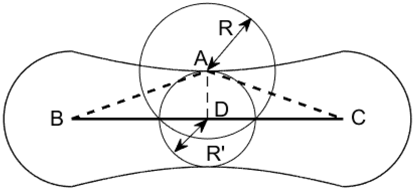
Spatial uncertainty is a non-negligible attribute of spatial data throughout their whole lifecycle. In a simple example shown in Figure 2, the original linear feature contains three vertices: B, A, and C. After generalization, vertex A is simplified, namely, the linear feature BAC becomes BC. Assume BAC to be the observed data with spatial uncertainty $u_o$ obeying a two-dimensional normal distribution where the probability distributions in x and y directions are independent and identical. Then, the uncertainty region of BC can be drawn using the error-band model.

Obviously, this model considers the spatial uncertainty of vertices larger than that of intermediate points. The uncertainty region of A is shown by $\odot \mathrm{A}$ centered on A with a radius of R, where R is a function related to the uncertainty model used (standard deviation, limit deviation, etc.) and the corresponding uncertainty value. After generalization, vertex A is mapped to an intermediate point D in BC, whose uncertainty is shown by $\odot \mathrm{D}$ centered on D with a radius of R’, where $\mathrm{R}\prime$ is equal to the width of the error-band at D. In fact, as there is a certain degree of deviation from vertex A to point D, the uncertainty of point D should be larger than that of vertex A. However, the area of $\odot \mathrm{D}$ and $\odot \mathrm{A}$ meets $Are{a}_{\odot \mathrm{D}}<Are{a}_{\odot \mathrm{A}}=Are{a}_{\odot \mathrm{B}}=Are{a}_{\odot \mathrm{C}}$, which means that the error-band model is not applicable for simplified linear features. As the same conclusion regarding other uncertainty models for linear features can be obtained in a similar way, the derivation process is not shown in this paper.

Almost all uncertainty models use error at a certain confidence level $\alpha$ with a distribution that is approximately normal to record spatial uncertainty. Let $Z_i=(x_i,y_i,{\sigma }_x,{\sigma }_y,\alpha )$ be a vertex in a linear feature in 2-D GIS and $Z_i^{\prime }=(x_i^{\prime },y_i^{\prime })$ be the corresponding vertex in the simplified feature, where ${\sigma }_x$ stands for error in the x direction, ${\sigma }_y$ stands for error in the y direction, and $\rho$ stands for the correlation coefficient between ${\sigma }_x,{\sigma }_y$.

Thus, the probability density function(pdf) of $Z_i$: $f_{Z_i}$ meets

$$f_{Z_i}={(2\pi {\sigma }_x{\sigma }_y\sqrt{1-{\rho }^2})}^{-1}\exp [-\frac{1}{2(1-{\rho }^2)}(\frac{{(x-x_i)}^2}{{\sigma }_x^2}-\frac{2\rho (x-x_i)(y-y_i)}{{\sigma }_x{\sigma }_y}+\frac{{(y-y_i)}^2}{{\sigma }_y^2})].$$

(13)

To ensure the same structure of uncertainty model between $Z_i$ and $Z_i^{\prime }$, let the pdf of $Z_i^{\prime }$ be

$$f_{Z_i^{\prime }}={(2\pi {\sigma }_x{\sigma }_y\sqrt{1-{\rho }^2})}^{-1}\exp [-\frac{1}{2(1-{\rho }^2)}(\frac{{(x-x_i^{\prime })}^2}{{\sigma }_x^2}-\frac{2\rho (x-x_i^{\prime })(y-y_i^{\prime })}{{\sigma }_x{\sigma }_y}+\frac{{(y-y_i^{\prime })}^2}{{\sigma }_y^2})].$$

(14)

Correspondingly, the marginal probability density functions (mpdf) of $Z_i$ and $Z_i^{\prime }$ are

$$\{\begin{array}{c}f{(x)}_{Z_i}=\frac{1}{\sqrt{2\pi }{\sigma }_x}{e}^{-\frac{{(x-x_i)}^2}{2{\sigma }_x^2}}\\ f{(y)}_{Z_i}=\frac{1}{\sqrt{2\pi }{\sigma }_y}{e}^{-\frac{{(y-y_i)}^2}{2{\sigma }_y^2}}\end{array},$$

(15)

respectively.

Accordingly, we have

$$D(Z_i;Z_i^{\prime })={{\displaystyle \sum }}_{x\in X}p(Z_i)\log \frac{p(Z_i)}{p(Z_i^{\prime })}={{\displaystyle \sum }}_{Z_i\in Z,Z_i^{\prime }\in Z^{\prime }}{f}_{Z_i}\log \frac{f_{Z_i}}{f_{Z_i^{\prime }}}.$$

(16)

In fact, available GIS uses just one parameter to describe the uncertainty of the point, that is, the long axis of the error ellipse, namely, ${\sigma }_Z=k\ast \max ({\sigma }_x,{\sigma }_y)$, where $k$ is a corresponding parameter at confidence level $\alpha$.

Obviously, this model of spatial uncertainty is relatively conservative and involves the following assumptions:

• The uncertainties in the x and y directions are independent of each other, namely, ${\rho }_{xy}=0$.
• The standard deviations in the x and y directions are equal to each other, namely, ${\sigma }_x={\sigma }_y={\sigma }_Z$.
  Thus, we have

  $$f_{Z_i}={(2\pi {\sigma }^2)}^{-1}\exp [-\frac{1}{2}(\frac{{(x-x_i)}^2}{{\sigma }^2}+\frac{{(y-y_i)}^2}{{\sigma }^2})]$$

  (17)

  $$f_{Z_i^{\prime }}={(2\pi {\sigma }^2)}^{-1}\exp [-\frac{1}{2}(\frac{{(x-x_i^{\prime })}^2}{{\sigma }^2}-+\frac{{(y-y_i^{\prime })}^2}{{\sigma }^2})].$$

  (18)

Generally, any point $z_i$ in a certain linear feature $z_0{z}_1$ can be represented as

$$\{\begin{array}{c}{x}_i=(1-r)x_0+r{x}_1\\ y_i=(1-r)y_0+r{y}_1\end{array},$$

(19)

where $r=S_i/S$, $S_i$ is the distance between $z_i$ and $z_0$, $S$ is the length of straight line $z_0{z}_1$, $\mathrm{and}(x_0,y_0)$,$(x_1,y_1)$, $(x_i,y_i)$ are the coordinates of point $z_0,z_1,z_i$, respectively.

According to the error propagation law, the uncertainty of point $z_i$ meets

$$\{\begin{array}{c}{\sigma }_{x_i}=\sqrt{{(1-r)}^2{\sigma }_{x_0}^2+r^2{\sigma }_{x_1}^2+2r(1-r){\sigma }_{x_0{x}_1}}\\ {\sigma }_{y_i}=\sqrt{{(1-r)}^2{\sigma }_{y_0}^2+r^2{\sigma }_{y_1}^2+2r(1-r){\sigma }_{y_0{y}_1}}\end{array}.$$

(20)

In consideration of the assumptions widely adopted in spatial uncertainty models, every vertex in the same linear feature follows the same pdf, which meets the attributes of isotropy, namely,

$${\sigma }_{x_0}^2={\sigma }_{x_1}^2={\sigma }_{y_0}^2={\sigma }_{y_1}^2,{\sigma }_{x_0{x}_1}={\sigma }_{y_0{y}_1}=0.$$

(21)

Thus, if ${\sigma }_Z$ is the standard error of vertices in linear feature $z_0{z}_1$, the uncertainty of any point in $z_0{z}_1$ can be simplified as

$$\{\begin{array}{c}{\sigma }_{x_i}=\sqrt{1-2r+2r^2}{\sigma }_Z\\ {\sigma }_{y_i}=\sqrt{1-2r+2r^2}{\sigma }_Z\end{array}.$$

(22)

Therefore, any point $Z_i$ in linear feature $z_0{z}_1$ meets

$${\sigma }_{Z_i}=k\ast \sqrt{1-2r+2r^2}\ast \max ({\sigma }_x,{\sigma }_y)=\sqrt{1-2r+2r^2}\ast {\sigma }_Z.$$

(23)

The spatial uncertainty model can be divided into the following categories according to the different values of k as shown in

Table 3. Different values of $k.$

Name of Error Model	Value of $\mathit{k}$	Probability in the Model (%)
Standard error	1.0	80.77
Probable error	0.5515	50
Epsilon accuracy	1.24	90
Circular error	1.96	95
Error entropy	2.332	99.87
Limit error	3.0	99.99

.

In the real GIS environment, the value of k usually is set to 3 [28,29]; therefore, this paper uses limit error to measure the spatial uncertainty.

According to the basic premise of a 1-D random variable, the radius of the uncertainty area of a 2-D normal random variable (point in 2-D environment) under confidence level $\alpha =99.99\%$ meets:

$$r_{UN}=\sqrt{\frac{{\sigma }_x{\sigma }_y\sqrt{(1-{\rho }^2)}(3^2\pi )}{\pi }}=3\ast \sqrt{{\sigma }_x{\sigma }_y\sqrt{(1-{\rho }^2)}}$$

(24)

$r_{UN}$ above can be simplified as $r_{UN}=3\sigma$ according to the limit error model widely adopted in spatial uncertainty models.

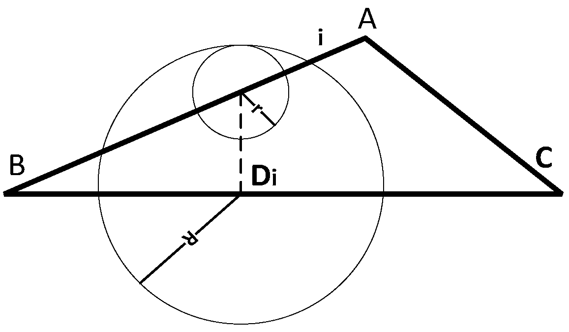
As shown in Figure 3, the linear feature before simplification is $L_0=\left\{B,A,C\right\}$ and the corresponding simplified feature is $L_1=\left\{B,C\right\}$. Let $i$ be any point in $L_0$, $D_i$ be the pedal on $L_1$ of $i$, $\mathrm{and}\odot i,\odot D_i$ be the circle with the radius $r_{UN}=3\sigma$ centered on point $i,D_i$.

In consideration of linear feature representing its corresponding geo-spatial entity’s location in the 2-D (or 3-D in 3-D GIS) space, the area inside $\odot i$ is the highly probably region ($p(\odot \mathrm{i})=99.99\%$), where the true value of $i$ lies. Thus, $\odot i$ can be considered an accurate representation of uncertainty within vertex $i$.

Obviously, the uncertainty model for every point $D_i$ in the simplified linear feature consists of two parts: the relative position relation vector $d_{i{D}_i}$ between $D_i$ and its corresponding point $i$ and the uncertainty $r_{U{N}_i}$ of point $i$ under a certain confidence level $\alpha$. Thus, the uncertainty of corresponding point $D_i$ can be obtained by

$$U_{D_i}=d_{i{D}_i}+r_{U{N}_i},$$

(25)

where $d_{i{D}_i}=(d_{\Delta x},d_{\Delta y})\mathrm{and}{r}_{U{N}_i}=(\alpha ,{\sigma }_i)$. As the uncertainty metadata of current spatial data contain only one element, the uncertainty of $D_i$ can also be the integration of $d_{i{D}_i},r_{U{N}_i}$, namely,

$$U_{D_i}=\left|d_{i{D}_i}\right|+r_{U{N}_i}.$$

(26)

Thus, the average uncertainty of the simplified straight line segment $L^{\prime }$ can be obtained by

$$U_{L^{\prime }}={{\displaystyle \sum }}_{D_i\in L^{\prime },i\in L}\frac{\left|d_{i{D}_i}\right|+r_{U{N}_i}}{point-number},$$

(27)

where $point-number$ stands for the total number of points participating the calculation.

In fact, as the circle $\odot D_i$ with the radius $U_{D_i}$ centered on point $D_i$ has the attribution of the inclusion of the circle with the radius $U_i$ centered on point $i$, the confidence level corresponding to $\odot D_i$ meets $\alpha \le {\alpha }^{\prime }\le 100\%$, demonstrating that this uncertainty calculation is a relatively conservative index.

3.4. Uncertainty Assessment of Linear Feature Simplification Based on Hierarchical Representation

As described in Section 3.2, linear feature $L_B$ and its simplified version $L_A$ can be represented as $L_B=\left\{L_{B0},L_{B1},\dots ,L_{Bb}\right\}\mathrm{and}{L}_A=\left\{L_{A0},L_{A1},\dots ,L_{Aa}\right\}$, respectively.

According to the hierarchical representation of $L_B,L_A$, a comparison between $L_B,L_A$ is made following the order of $L_0\to L_{max}$. Let the earliest level of difference be $L_i$($L_{Ai},L_{Bi}$), with the difference element represented by $F_i$. Obviously, $L_i$ forms the most abstract different level of $L_B$ and $L_A$ and shows the greatest impact on simplification of $L_B$ to $L_A$. Further, the subtree of $F_i$ must be different, which has a lesser impact than $F_i$; thus, the assessment terminates at $F_i$.

Let the parent node of $F_i,F_{i^{\prime }}$ be $F{F}_i=\left\{F{L}_1,F{L}_2,\dots \right\}\mathrm{and}F{F}_{i^{\prime }}=\left\{F{L}_{1^{\prime }},F{L}_{2^{\prime }},\dots \right\}$. Obviously, we have $L_1=L_{1^{\prime }};L_2=L_{2^{\prime }}$ and $F_i\ne F_{i^{\prime }}.$

Depending on relationship between $F_{i^{\prime }},F_i$, that is, whether proposition $F_{i^{\prime }}\subseteq F_i$ is true or not, the condition can be divided to 2 cases:

Case 1. $F_{i^{\prime }}\subseteq F_i$. In this case, the simplified linear feature $L_A$ has a loss of partial feature vertices in level $F_{i^{\prime }}$, resulting in $F_{i^{\prime }}$ being null (its parent node being a leaf node). The formal description as follows: $\exists F{L}_{i^{\prime }}\in F{F}_{i^{\prime }}$, meets the following:

• $F{L}_{i^{\prime }}$ is a leaf node.
• Its corresponding node in the original linear feature $F{L}_i$ is not a leaf node.

Thus, the computation of spatial uncertainty can be transformed into a typical 1: n relationship between $F{L}_i$ and its child nodes.

A diagram of Case 1 is given in Figure 3. In the diagram, leaf node $F{L}_{i^{\prime }}$ is represented by straight line segment BC, while in the same node in the corresponding DMC-Tree of the original linear feature, $F{L}_i$ has child nodes BA and AC. Thus, the computation of uncertainty caused by simplification can be transformed to the difference from BA and AC to the single straight line segment BC.

By regarding line segments BAC and BC as innumerable points, we can construct the mapping relation between them. For any point $i$ in BAC, its corresponding point $D_i$ is its pedal in a vertical line normal to BC. Obviously, the length of straight line segment $i{D}_i$ is equal to the distance between point $i$ and straight line through BC. With circle $\odot i$ with the radius $r$ representing its spatial uncertainty, centered on point $i$, the spatial uncertainty of point $D_i$ is then the minimum radius of circle $\odot D_i$ centered on point $D_i$ meeting $\odot i\subseteq \odot D_i$.

Thus, the average spatial uncertainty of node BC in DMC-Tree can be computed as

$$U_{BC}=\frac{1}{n}{\displaystyle \sum _{i=1}^n{R}_i},$$

(28)

where n is the total number of points in BC.

Case 2. $F_i\not\subset F_{i^{\prime }}$. In this case, the simplified linear feature $L_A$ has some different vertices with $L_B$ in level $F_{i^{\prime }}$, while $F{F}_{i^{\prime }}$ is not a leaf node.

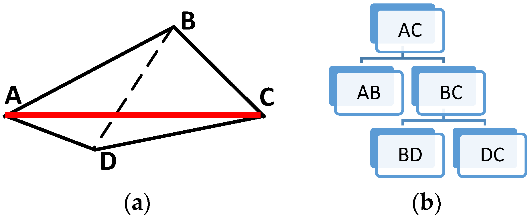
A diagram of Case 2 is given in Figure 4, where the original curve is ABDC.

In Figure 4, line segment AB, BC represents $F_i$, and AD, DC represents $F_{i^{\prime }}$. The simplification of linear feature $L_B$ losses feature vertex B in level $L_i$, resulting in D as its corresponding vertice, while in the original linear feature, D exists in a deeper level.

Obviously, as a result of the difference between characteristic points (B, D), the morphological difference here is larger than that in Case 1. When the same method in Case 1 is used to construct the mapping relation between ABC and ADC, there may be some points in ABC with no corresponding points in ADC.

The computation of spatial uncertainty in Case 2 is given below:

• Connecting the common endpoints (A, C) and importing the method in Case 1 to map all the points along both ABC and ADC to straight line AC.
• Let $f(·),g(·)$ be the map function from ABC and ADC to AC, respectively. Map function $F(P):ABC\to ADC$ is constructed by using transitivity in the map function, namely,

  $$\forall P_z\in ABC,\exists |Q_z\in ADC,\mathrm{meets}(1)F(P_z)=Q_z;(2)f(P_z)=g(Q_z)=A{C}_z.$$

Thus, the average spatial uncertainty of simplified line ADC can be computed as

$$A{U}_{ADC}=\frac{1}{m}{{\displaystyle \sum }}_{i=1}^m{R}_i,$$

(29)

where m is the total number of points in AC.

At this point, the transformation of spatial uncertainty caused by simplification in a certain level of DMC-Tree is complete. For the computation of the whole linear feature, answers of all levels should be integrated together.

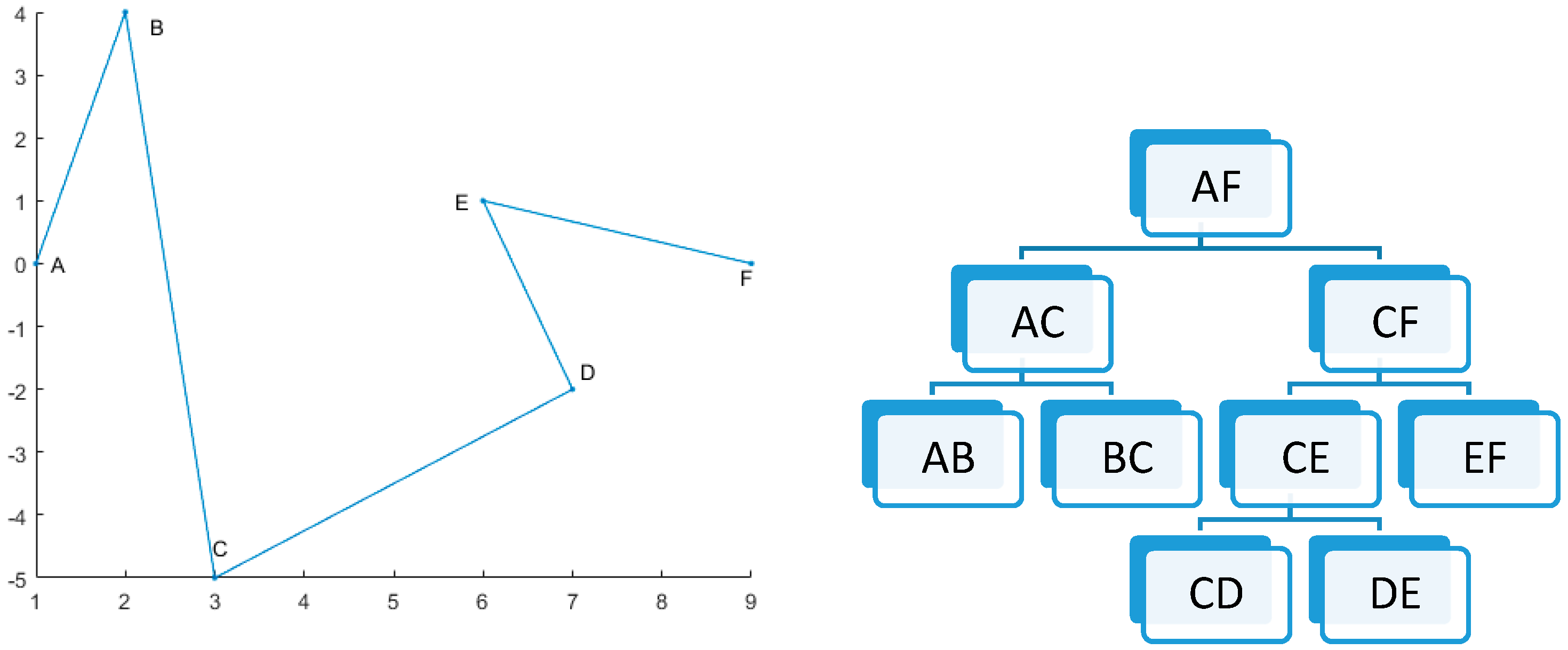
A typical structure in a DMC-Tree is shown in Figure 5.

Let $\left|B\right|$ be the length of straight line segment B. Considering the geographical feature of the linear feature and the hierarchical structure of its corresponding DMC-Tree, the longer the straight line segment is, as well as the higher the level is, the more important it is in GIS databases and products. As a result, the weight assignment model is designed as follows:

• The weight of root node is set to be 1.
• Weights of child nodes are inherited from their parent node.
• Weights between sibling nodes are prorated by their length.

As for the upper diagram, we have

$${\omega }_A+{\omega }_C={\omega }_B$$

(30)

$${\omega }_A={\omega }_B·\frac{\left|A\right|}{\left|A\right|+\left|C\right|}.$$

(31)

3.5. Complexity Analysis of the Algorithm

3.5.1. Analysis of the Time Complexity

The whole algorithm can be divided into 2 parts:

Part 1. Construction of DMC-Tree

In this part, the algorithm runs like the classic Douglas-Peucker algorithm, with its time complexity as O(nlogn).

Part 2. Computation of spatial uncertainty in each level.

Depending on the location and number of difference in DMC-Tree between both linear features, the time complexity of this part varies from O(n) all the way up to O(logn). In detail,

O(n): Simplification causes a loss of some very important vertices (for example, certain vertices in the first level under extreme circumstances);

O(nlogn): Simplification only causes a loss of some least important vertices (for example, certain vertices in the deepest level under extreme circumstances);

In conclusion, the overall time complexity of the algorithm remains O(nlogn).

3.5.2. Analysis of the Space Complexity

The storage space needed in the multi-scale spatial uncertainty method includes (1) storage used by the DMC-Tree, the size of which is nlogn, where n represents the vertex number in the corresponding linear feature, and (2) storage used by the quality of all the vertices, the size of which is n. Thus, the storage space needed in this method is nlogn.

4. Experiments

To validate the availability, correctness and advantages of the multi-scale spatial uncertainty method among widespread methods, namely, the length ratio method and the Hausdorff distance method, several experiments were designed on both simulated data and real data. A prototype system was developed using C++ and Visual Studio 2010.

4.1. Experiments on Simulated Data

First, three quality assessment methods are preliminarily verified by one group of experiments on simulated data.

There are six vertices in the simulated data: one starting point, one endpoint, and four intermediate points. Here, four intermediate vertices are deleted to simulate different results of the linear feature simplification one at a time, as is shown in Figure 6, and the uncertainties of all vertices are set to be 1.

Quality assessment results of this group of experiments are shown in

Table 4. Quality assessment results of experiments on simulated data.

	Methods	Multi-Scale Spatial Uncertainty			Length Ratio	Hausdorff Distance	Location Error
Curve		Maximum Uncertainty	Highest Level/Vertex	Average Uncertainty	Ratio	Distance	Mean Distance
Original		1	NULL	0.811936	100%	0	0
Without B		6.571951	2/B	1.949738	68.19%	4.1231	0.2652
Without C		9.428571	1/C	5.306216	74.51%	5	0.7958
Without D		3.234523	3/D	1.261412	94.07%	2.8284	0.3061
Without E		3.837152	2/E	1.682238	85.73%	3.1623	0.1632

, where the maximum uncertainty and average uncertainty means the maximum and average uncertainty of all vertices, respectively.

Visually, the deletion of vertex C causes the greatest impact on shape of the curve, followed by the deletion of vertex B, while the impact of deleting vertices D or E is relatively slight. The results of three quality assessment methods but the LEM (whose order is: E > B > D > C) follow the same quality order, namely, D > E > B > C, also in accordance with human visual perception. Thus, the Location Error Model is no longer used in the following experiments.

While focusing on the curve without B and the curve without C, the difference between quality index of length ratios (68.19% vs. 74.51%) and Hausdorff distances (4.12 vs. 5) is rather small, while the difference in the multi-scale spatial uncertainty (1.95 vs. 5.31) is quite significant. This phenomenon indicates the advantage of MS2U in detecting the loss of main feature points. The outputs of MS2U also include the maximum uncertainty and its corresponding level and vertex, providing quality metadata for the simplified linear feature under multiple scales for cartographic generalization with vertex granularity.

4.2. Experiments on Real Data

As shown in Figure 7, a segment of a hydroline of 100 vertices and a boundary line of 200 vertices from the Digital Atlas of the Earth (DAE) are used as the original linear feature in the experiments in this section. The spatial uncertainty of these features is considered to be $\pm 50\mathrm{m}$ (or $0.00045°$ in the geographic coordinate system). These linear features are chosen as representative of linear natural entities and linear artificial entities, respectively.

Visually, the overall shape of the hydroline is more complex (many irregular bends exist) than that of the boundary (overall stable with few drastic changing intervals). Thus, the complexity of these linear features has certain representativeness in both natural and artificial linear features.

In this section, the Douglas–Peucker algorithm (DPA) and the vertical distance algorithm (VDA) are used for the simplification of linear features. The outputs of DPA and VDA with 50% and 25% vertices retained are used as the simplified linear feature; the corresponding tolerances are shown in

Table 5. Relationship between tolerances and ratio of vertices retained $(°).$

	Tolerances
	Hydroline		Boundary Line
Ratio Retained	50%	25%	50%	25%
Douglas–Peucker Algorithm	0.000135	0.000340	0.000136	0.000423
Vertical Distance Algorithm	0.000125	0.000258	0.000112	0.000260

.

In the next few sections, the linear features used (a hydroline, a boundary and their corresponding simplified versions) are shown with the original line features in blue and the simplified versions in red.

4.2.1. Simplifications by DPA

As shown in Figure 8 and Figure 9, the hydroline and boundary are simplified by DPA with vertices retained at 50% and 25%, respectively.

1. Hydroline (Ratio of Vertices Retained 50%, 25%)

As the contributing factor of a river is rather complicated, the shape of the hydroline is irregular and complex, making the simplification somewhat difficult. Visually, the left hydroline in red reserves more details (looks almost the same in total as the original hydroline with a few small distinctions) than the right one (lost some small but identifiable shapes). Obviously, the similarity between linear features decreases with a decrease in the ratio of vertices.

2. Boundary Line (Ratio of Vertices Retained 50% and 25%)

Compared with the hydroline shown in Figure 10, the boundary used here is formed by twice the number of vertices of the hydroline, while it can be spliced into two types of sections, namely, sharp corner sections and smooth linear sections. Because the boundary used here includes twice the number of vertices of the hydroline, both the simplified boundary lines are more similar to the original boundary line, with the most obvious difference in the turning points in the right fig, visually.

4.2.2. Simplifications by VDA

As shown in Figure 10 and Figure 11, the hydroline and boundary are simplified by VDA with vertices retained at 50% and 25%, respectively.

1. Hydroline (Ratio of Vertices Retained at 50% and 25%)

Visually, the hydroline simplified by VDA with vertices retained at levels of 50% and 25% also shares little difference with the original hydroline. However, when compared with that simplified by DPA, VDA clearly leads to a greater loss of detail, even feature points, than the DPA, especially in the right figure (several main feature points are lost).

2. Boundary Line (Ratio of Vertices Retained at 50% and 25%)

Similar to Figure 11, both the simplified boundary lines are more similar to the original boundary line than the hydroline simplified shown in Figure 12, with the most obvious difference in the turning points in the right figure, visually. When compared with that simplified by DPA, a greater loss of detail can be found in some of the sharp corners.

4.2.3. Simplifications for Different Linear Features

In this sub–subsection, different types of linear features, namely, hydrolines, boundaries of one marshland and roads from DAE and contour lines derived from the National Centers for Environmental Information’s DEM, are used as the original linear feature to test the usability of the method presented, as shown in

Table 6. Linear features used to verify the usability of MS2U.

Linear Feature Used	Number of Lines	Spatial Error
Hydroline	100	$0.00045°$
Boundary	100	$0.00045°$
Contour line	100	$\pm 25\mathrm{m}$
Road	100	$0.00045°$

, with a visual representation in Figure 12.

In this sub–subsection, every linear feature in the area is cut into segments consisting of 100 vertices to run the experiment. All these linear features are simplified by DPA to run the quality assessment. Visually, bends in the roads are the least, followed by the contour lines. Bends in the boundaries are the most inhomogeneous (as parts of them are natural, while some are artificial), while the hydrolines are the most complex because of their huge number of small bends.

4.3. Quality Assessment Results

To verify the method, experiments were conducted to provide a comparison with the widely used length ratio method and Hausdorff distance method. The main results are discussed below.

4.3.1. Contrast between DPA and VDA

The comparison between two simplification algorithms DPA and VDA is shown in

Table 7. Quality assessment results of simplification by DPA.

Linear Features		Number of Vertices	Quality Assessment Methods
			Length Ratio	Hausdorff Distance (${10}^{-4}°$)	Average/Max Uncertainty (${10}^{-4}°$)
Hydroline	Original	100	100%	0	3.65/4.5
	50% retained	50	98.81%	15	3.96/5.83
	25% retained	25	96.02%	40	4.69/7.87
Boundary	Original	200	100%	0	3.65/4.5
	50% retained	100	99.94%	54	3.91/5.86
	25% retained	50	99.63%	97	4.69/8.72

and

Table 8. Quality assessment results of simplification by VDA.

Linear Features		Number of Vertices	Quality Assessment Methods
			Length Ratio	Hausdorff Distance (${10}^{-4}°$)	Average/Max Uncertainty (${10}^{-4}°$)
Hydroline	Original	100	100%	0	3.65/4.5
	50% retained	50	96.17%	14	29.82/56.71
	25% retained	25	96.02%	49	29.20/55.34
Boundary	Original	200	100%	0	3.65/4.5
	50% retained	100	98.67%	72	27.65/55.02
	25% retained	50	97.83%	116	24.56/39.38

.

As we can see, with the decrease in the number of vertices retained, the results of all the quality assessment methods decrease to some extent. Thus, the correctness of these methods is preliminarily validated.

Theoretically, the differences between DPA and VDA can be summarized as follows:

• Preservation of feature points
  The DPA can preserve the feature points in the upper layers of the DMC-Tree, while the VDA does not take feature points into account strictly.
• Preservation of details
  As all the details with distance to the baseline shorter than the threshold set in DPA will be simplified; details preserved by DPA are relatively few, while the VDA performs better in this task. The same conclusion can be obtained visually.

1. Simplification by DPA

Analyzing the results of all three assessment methods reveals that the change in length ratio of the boundary remains very slight, which is in accordance with people’s visual cognition. Under the same condition, the results of the Hausdorff distance method show that the simplified boundary with 50% vertices retained has a larger distance than that with 25% vertices retained. By comparing the corresponding pair of boundary data, one vector of larger distance to the other boundary is found. This phenomenon shows that the Hausdorff distance method is sensitive to extreme points.

Overall, the quality variation during simplification stays relatively low, showing that the Douglas–Peucker algorithm retains the main shape feature and location accuracy of the linear feature effectively.

2. Simplification by VDA

Visually, the results of VDA have a greater degree of loss in main shape and feature points; thus, quality assessments should reveal a lower quality of VDA than of DPA.

Linear features simplified by VDA share some characteristics in common with linear features simplified by DPA: (1) the results of all the quality assessment methods decrease as the number of vertices retained decreases; (2) the length ratio shows a higher quality of boundary used in both scales, while the Hausdorff distance shows a higher quality of hydrolines used in both scales.

A strange phenomenon exists in which the simplified linear feature with 50% vertices retained scored a lower result than that with 25% vertices retained. To further examine this phenomenon, structure differences of the corresponding DMC-Trees were checked from the top down, revealing that VDA leads to a loss of one feature vertex in the 2nd layer, which in turn leads to a worse result. As the results show, almost all quality indexes of all scales on both linear features show a worse quality of the vertical distance algorithm (except a slightly better Hausdorff distance of hydroline with 50% vertices retained (15 vs. 14)). The average and max uncertainty indexes are much worse than those of the DPA. Overall, the quality variation during simplification is rather unstable for different linear features, showing that the use of the vertical distance algorithm may be taken into careful consideration.

4.3.2. Contrast between Different Scales

As the conclusion in upper sections shows that the VDA has a greater influence than the DPA in both main shape and feature vertices, the contrast experiments between different scales are conducted on DPA.

Here, the ratio of vertices retained is used as the representation for scale. Quality assessment methods are used for nine different ratios of vertices retained, as shown in

Table 9. Quality assessments for hydroline.

	Vertices Retained	90%	80%	70%	60%	50%	40%	30%	20%	10%
Quality Indexes
Length Ratio (100%)		99.92	99.74	99.5	99.3	98.81	97.99	96.79	95.19	92.12
Hausdorff Distance (10−4$°$)		8.44	8.81	8.81	13	15	17	17	46	46
Average Uncertainty (10−4$°$)		3.68	3.7	3.74	3.84	3.96	4.13	4.38	5	6.02
Max Uncertainty (10−4$°$)		5.01	5.09	5.17	5.46	5.83	6.46	6.97	8.39	10.55

and

Table 10. Quality assessments for boundary.

	Vertices Retained	90%	80%	70%	60%	50%	40%	30%	20%	10%
Quality Indexes
Length Ratio (100%)		99.99	99.99	99.99	99.97	99.94	99.87	99.73	99.43	98.21
Hausdorff Distance (10−4$°$)		30	35	45	54	54	83	97	108	222
Average Uncertainty (10−4$°$)		3.65	3.67	3.71	3.78	3.91	4.09	4.36	5.16	8.8
Max Uncertainty (10−4$°$)		4.53	4.76	4.97	5.34	5.86	6.39	7.61	10.15	22.46

.

1. Hydroline

2. Boundary

The span between the original scale and the target scale clearly affects the quality of simplification. Theoretically, in the linear feature simplification, the smaller the scale is, the fewer vertices retained, the greater the information loss. However, the effect of scale on simplification is not linear: the larger the scale span is, the faster the information is lost.

Visually, the differences between linear features expand when the scale decreases, leading to more significant differences between them. The results presented here reveal that the quality indexes decline in almost all cases when the scale decreases, except for only one case: quality indexes for a hydroline simplified by VDA between the ratio of vertices retained by 50% and 25%. Checking the corresponding linear feature reveals that VDA leads to a loss of one feature vertex in the 2nd layer, which in turn causes this unusual result.

4.3.3. Contrast between Different Linear Features

All these linear features are simplified by DPA, with 50% and 25% vertices retained. Indexes including average maximum spatial uncertainty, average spatial uncertainty, length ratio and Hausdorff distance are used to show the simplification results, as shown in

Table 11. Linear features simplified by DPA with 50% vertices retained.

	Methods	Multi-Scale Spatial Uncertainty		Average Length Ratio	Average Hausdorff Distance
Features		Average Maximum Uncertainty	Average Uncertainty	Ratio	Distance
Hydroline (${10}^{-4}°$)		$11.38$	$4.18$	98.29%	14.92
Boundary (${10}^{-4}°$)		$11.81$	4.95	98.95%	17.83
Contour line (m)		11.63	4.12	98.51%	17.82
Road (${10}^{-4}°$)		8.23	3.26	99.97%	9.69

and

Table 12. :Linear features simplified by DPA with 25% vertices retained.

	Methods	Multi-Scale Spatial Uncertainty		Average Length Ratio	Average Hausdorff Distance
Features		Average Maximum Uncertainty	Average Uncertainty	Ratio	Distance
Hydroline (${10}^{-4}°$)		14.35	6.41	96.33%	43.59
Boundary (${10}^{-4}°$)		13.29	5.64	96.54%	42.66
Contour line (m)		14.27	6.30	95.83%	41.75
Road (${10}^{-4}°$)		12.52	4.41	99.66%	25.72

.

Overall, the span between the original scale and the target scale clearly affects the quality of simplification significantly; all indexes of all linear features with 25% vertices retained are lower than that of 50% vertices retained. Specifically, the simplification quality of roads outperforms other linear features, showing that the quality of simplification is positively related to the complexity of the linear feature under the same simplification degree, which is also in accordance with human cognition. However, spatial uncertainty obtained by the method presented in this paper is consistent with that of the other two methods, showing its usability for different linear features.

4.4. Discussion

By regarding the linear feature as a whole, the length ratio method provides a kind of coarse-grained simplification method, whose advantages lie in its easy implementation, low computation cost and robustness. The widely used Hausdorff distance method also regards the linear feature as a whole to assess the quality of linear feature simplification, and its advantage lies in its wide applicability. Compared with the traditional Euclidean distance method, Hausdorff distance has the ability to calculate the line-line distance of any pair of intersecting lines. However, as the Hausdorff distance is determined solely by the maximum of the distance between all the vertices on the line segments, it is vulnerable to outliers.

By comparison, the MS2U method takes full account of features (feature points and spatial uncertainty) of linear feature and its simplification (multi-scale consistency), thus drawing a more objective conclusion (e.g., the quality assessment results of the Hausdorff distance method and MS2U on 50% and 25% vertices retained by VDA).

On the other hand, the MS2U method has the ability above the other two methods mentioned above in computing the spatial uncertainty of any point, rather than just vertices, in any scale, which provides the ability for getting the quality distribution along the whole linear feature.

5. Conclusions

The importance of quality assessment for linear feature simplification is increasingly important for both geographers and customers. Thus, in this study, we introduced the quality assessment method for linear feature simplification based on multi-scale spatial uncertainty (MS2U).

In this method, a hierarchical representation of linear feature is proposed by reorganizing the linear feature to a weighted multiway tree, DMC-Tree. Then, the spatial error of the original linear feature and the spatial location deviation caused by simplification are integrated as the spatial uncertainty. By adjusting the scale parameter, this method can obtain spatial uncertainty of any point (rather than just vertices) under any scale, which is very useful for both geographers and users. Experiments on both simulated data and real data indicate the advantages of MS2U in granularity, objectivity and usability.

However, the proposed MS2U method still has its deficiency, namely the hypothesis of the strict reservation of start and end vertices. Once this hypothesis becomes false, the DMC-Tree structure will be totally changed from the root, making the match between linear features chaotic, which in turn biases the assessment results. Future studies may include quality assessment under such a circumstance.