A Map Spectrum-Based Spatiotemporal Clustering Method for GDP Variation Pattern Analysis Using Nighttime Light Images of the Wuhan Urban Agglomeration

Abstract

Estimates of gross domestic product (GDP) play a significant role in evaluating the economic performance of a country or region. Understanding the spatiotemporal process of GDP growth is important for estimating or monitoring the economic state of a region. Various GDP studies have been reported, and several studies have focused on spatiotemporal GDP variations. This study presents a map spectrum-based clustering approach to analyze the spatiotemporal variation patterns of GDP growth. First, a sequence of nighttime light images (from the Defense Meteorological Satellite Program-Operational Linescan System (DMSP-OLS)) is used to support the spatial distribution of statistical GDP data. Subsequently, the time spectrum of each spatial unit is generated using a time series of dasymetric GDP maps, and then the spatial units with similar time spectra are clustered into one class. Each category has a similar spatiotemporal GDP variation pattern. Finally, the proposed approach is applied to analyze the spatiotemporal patterns of GDP growth in the Wuhan urban agglomeration. The experimental results illustrated regional discrepancies of GDP growth existed in the study area.

1. Introduction

The spatiotemporal patterns of gross domestic product (GDP) are considered significant indicators when evaluating the economic status of a region. Such patterns are also important in decision making related to regional economic plans. Thus, obtaining the precise spatial distributions of GDP in a specific region at different times and analyzing the associated spatiotemporal processes are crucial for assessing the economic status and growth of a region. These elements are also crucial for precise regional planning and sustainable development. Specifically, it is a common and necessary practice to obtain dasymetric maps by mapping statistical socioeconomic data. For instance, to address the inadequacy of census data in reflecting the internal differences of populations in a given area, populations across China were interpolated using nighttime imagery and land use data [1]. To determine the spatial distributions of the physical, climatic, and socioeconomic aspects that best characterize the production of dairy goats and their impact on animal breeding decisions in Brazil, these statistical data were firstly mapped to dasymetric maps [2]. Cao et al. [3] estimated the spatial distribution and analyzed the spatiotemporal changes in electricity consumption from 1994 to 2009 in China. Silva et al. [4] used secondary data and the quantitative limits of the Institute of Technical–Scientific Policy and an areal interpolation method to acquire the spatiotemporal distribution of homicide cases in Mossoró City from 2010 to 2013. However, the interpolation theory is based on the assumption that the closer the point is, the more likely it is to have the same eigenvalues. Additionally, only a statistical GDP value is associated with an administrative unit and its precise position is not known. Therefore, such an interpolation method is inappropriate for obtaining a dasymetric map of GDP, which can reflect the internal differences between different areas in a region. In addition, this case suggests that a dasymetric map of GDP can be obtained based on the digital numbers (DNs) of calibrated night light images because these DNs reflect the levels of human activity, commercial activity, and industrial activity, which are related to GDP.

Various approaches to spatiotemporal analysis have been reported. The spatial and temporal variations in seismicity in the northwestern region of Iran were evaluated with a focus on seismic precursors on 11 August 2012, when the Mw 6.5 Varzeghan earthquake occurred [5]. Wang et al. [6] analyzed the spatial pattern of wildfire-related tweets based on kernel density estimation. Then, they analyzed the spatial and temporal relationship between social media activities and wildfire disruptions by evaluating the temporal evolution of wildfire-related tweets and examining whether clusters of wildfire-related tweets on the impacted areas had occurred. However, in these two cases, space and time were analyzed separately, and no spatiotemporal evolution model was proposed to analyze the spatiotemporal processes involved in the study. Based on a gridded dataset, hierarchical and non-hierarchical (k-means) clustering techniques were used to objectively and automatically delineate homogeneous precipitation regions with highly variable spatiotemporal patterns [7]. Zhang et al. [7] focused on determining an optimal k for k-means clustering. Vogel et al. [8] proposed a framework for the modeling, analysis, and simulation of aero-optic wave front aberrations. This approach was based on spatiotemporal covariance matrices, which were extracted from measured wavefront sensor data. Qian et al. [9] performed spatiotemporal analyses of surface coalmining-dominated land degradation in Holingol, Inner Mongolia. In this case, a grid square-based correlation was employed to investigate the correlations among mining area expansion, urban area expansion, and grassland change. The spatiotemporal dynamics of mines and urban growth patterns were obtained based on land use differences between two periods in each grid cell.

Moreover, as one of the primary approaches for spatiotemporal process analysis, spatiotemporal clustering has been reported in previous studies. Li et al. [10] evaluated the Syrian crisis using nighttime light images. In this case, a k-means clustering algorithm was used to obtain the light trend and associated spatial distribution. McArdle et al. [11] applied clustering techniques based on spatial and temporal similarity to mouse group trajectories with similar behavioral properties. Chidean et al. [12] applied a self-organized, second-order, data-coupled clustering algorithm to analyze the spatiotemporal patterns of temperature in Europe. Wu et al. [13] applied the Bregman block average co-clustering algorithm with I-divergence (BBAC_I) to an aggregated annual temperature data matrix to study the associated spatiotemporal patterns at an annual temporal resolution. Damiani et al. [14] proposed a recent time-aware, density-based clustering technique and used it to study partial migrations. In summary, these spatiotemporal analysis approaches commonly fail to effectively model spatiotemporally integrated processes. Thus, the relevant methods cannot be efficiently used to represent the spatiotemporal patterns of GDP evolution.

To investigate the characteristics of internal variations in GDP growth in the Wuhan urban agglomeration, GDP dasymetric maps of the study area from 1992 to 2012 were created using GDP statistical data and saturation-corrected nighttime light images obtained by the Defense Meteorological Satellite Program (DMSP)-Operational Linescan System (OLS). Additionally, a map spectrum-based, spatiotemporally integrated clustering model is proposed to classify the patterns of variation. The proposed model simultaneously considers both spatial and temporal characteristics in clustering and it differs from existing methods, in which spatial and temporal characteristics are considered separately in clustering. The results of this study show that the proposed model can reflect regional discrepancies in the variations of GDP growth, especially in the urban, suburban, and rural areas of the Wuhan urban agglomeration.

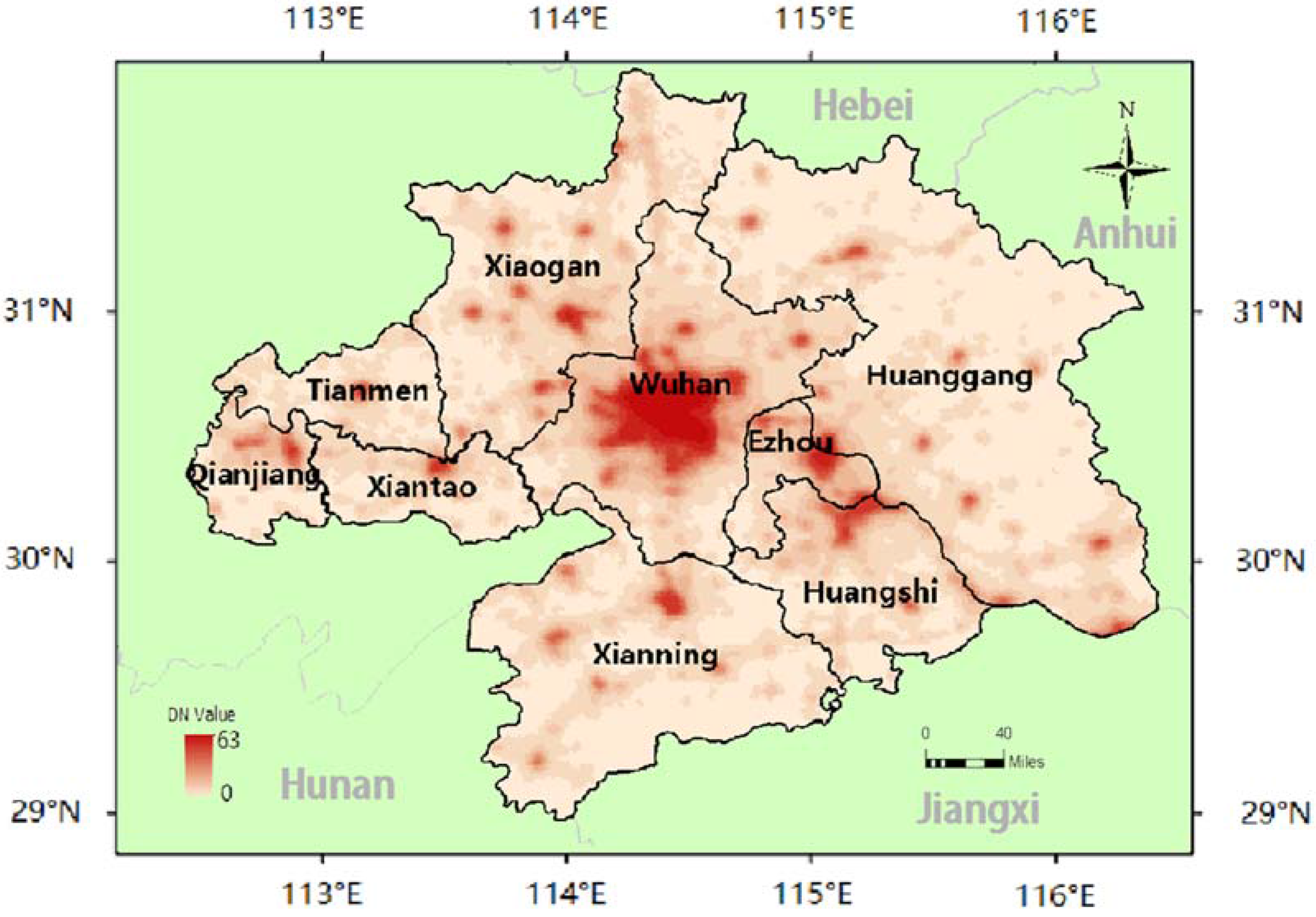
2. Study Area and Data

As a key metropolitan area in the central part of China, the Wuhan urban agglomeration, which includes nine prefectures, was selected to investigate the spatiotemporal variations in GDP development. This area is one of the largest city clusters in central China. Additionally, the agglomeration is not only the core of economic development in Hubei but is also an important strategic fulcrum for the rise of central China. Notably, it is the central node of the Yangtze River Economic Zone and plays an important role in linking the east and west and connecting the south and north in terms of economic development in China.

GDP statistical data and DMSP-OLS nighttime light data collected in the study area are used in this study. The GDP data from each prefecture in the Wuhan urban agglomeration were obtained from the statistical yearbook of the corresponding city from 1992 to 2012. Meanwhile, the two types of DMSP-OLS datasets used in this study were provided by the National Oceanic and Atmospheric Administration (NOAA)-National Geophysical Data Center (NGDC) [15]. The ‘Global DMSP-OLS Nighttime Light Time Series (Version 4)’ dataset, which includes non-radiance-calibrated (NRC) light intensity recorded as 6-bit DNs ranging from 0 (no light) to 63 (saturation) by averaging DN values of stable light images throughout the year, collected from 1992 to 2012 was used to create the dasymetric map of GDP. The ‘Global Radiance Calibrated Product’, which includes radiance-calibrated light intensity, from 2011 was used to correct saturation problems in the version 4 dataset. All these global datasets were extracted based on the boundary of the Wuhan urban agglomeration, reprojected to the Universal Transverse Mercator (UTM) North 49 projection with the WGS84 datum, and resampled to a 1 km grid. Figure 1 shows the NRC DMSP-OLS data from the Wuhan urban agglomeration in 2011.

Additionally, Chinese land use/cover data from 1995, 2000, 2005, and 2010, all with a spatial resolution of 1 km, were provided by the Data Center for Resources and Environmental Sciences of the Chinese Academy of Science [16]. These data were produced through visual interpretation of Landsat TM images [17]. This dataset was used as ancillary data in our study.

3. Dasymetric GDP Map Using Nighttime Light Images

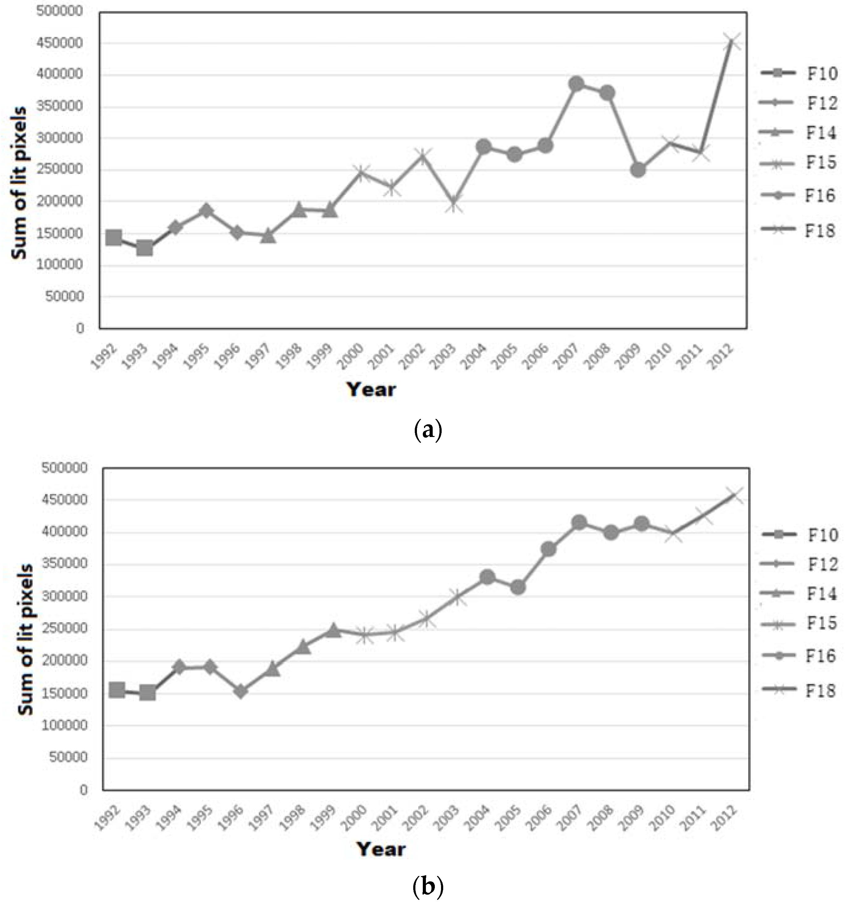
3.1. DMSP-OLS Data Preprocessing

NRC DMSP-OLS saturation data can underestimate the GDP values of saturated pixels and overestimate the values of non-saturated pixels. Lo [18] and Cao et al. [3] found that GDP is related to DMSP-OLS data in China. In the NRC DMSP-OLS dataset collected over the Wuhan urban agglomeration from 1992 to 2012, saturated pixels only existed in the data from 2010 to 2012. Therefore, the saturated pixels in NRC DMSP-OLS data were corrected by adopting the method developed by Cao et al. [3], RC DMSP-OLS data and prefectural GDP statistical data from the Wuhan urban agglomeration in 2011.

Figure 2 shows the linear relationship between GDP per km² and RC DMSP-OLS DN values per km² for 9 prefectures in 2011. This relationship was similar to those in other years in the Wuhan urban agglomeration area. In the Wuhan urban agglomeration, the GDP of Wuhan is much larger than those of other prefectures. To avoid overestimating the determination coefficient of the regression equation caused by uneven data distributions, the logarithms of the independent and dependent variables were used in the calculation. The NRC DMSP-OLS data can be corrected using the formula

D_{total_area} = a × GDP_area + b

(1)

where D_{total_area} is the logarithm of the corrected total DMSP-OLS DN values per km² in a prefecture with saturated pixels; GDP_area is the logarithm of the GDP per km² of the corresponding prefecture; and a and b are regression parameters, which are 0.63615 and −1.27474, respectively, in this study. The corrected values of saturated pixels can be calculated by subtracting the total DN of non-saturated pixels from the total corrected DN of the prefectural area and then dividing this value by the number of saturated pixels in the prefecture [3].

Due to a lack of on-board calibration and intercalibration, the inconsistencies between DMSP-OLS nighttime stable light data are obstacles in time series analysis. Therefore, the annual nighttime stable light data from different satellite missions were intercalibrated using the quadratic regression model (Equation (2)) proposed by Elvidge et al. [19]. The model parameters a_t, b_t, and c_t in each year t were obtained from a study by Liu and Li [20], who used nighttime stable light data from mission F16 in 2007 as a baseline and performed quadratic regressions in invariant areas with little change in actual DNs over time. In addition, the pixels with zero values were excluded from the intercalibration.

DN’_t = a_t × DN²_t + b_t × DN_t + c_t

(2)

where DN’_t is the DN of a pixel after calibration in year t; DN_t is the original DN of a pixel in that year; and a_t, b_t and c_t are the corresponding model parameters. Figure 3 shows that the intercalibration improved the continuity of nighttime stable light data in study area from 1992 to 2012.

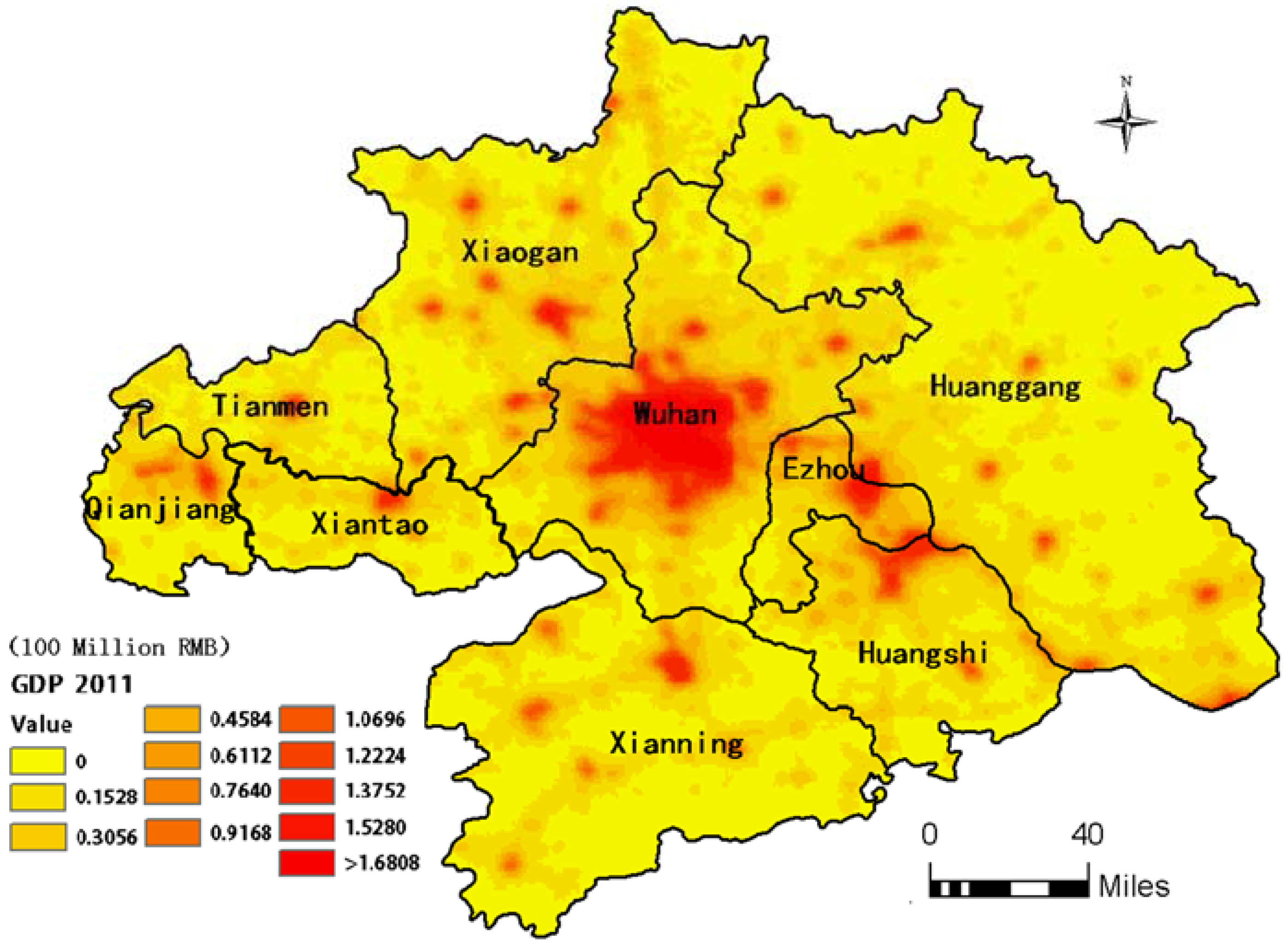
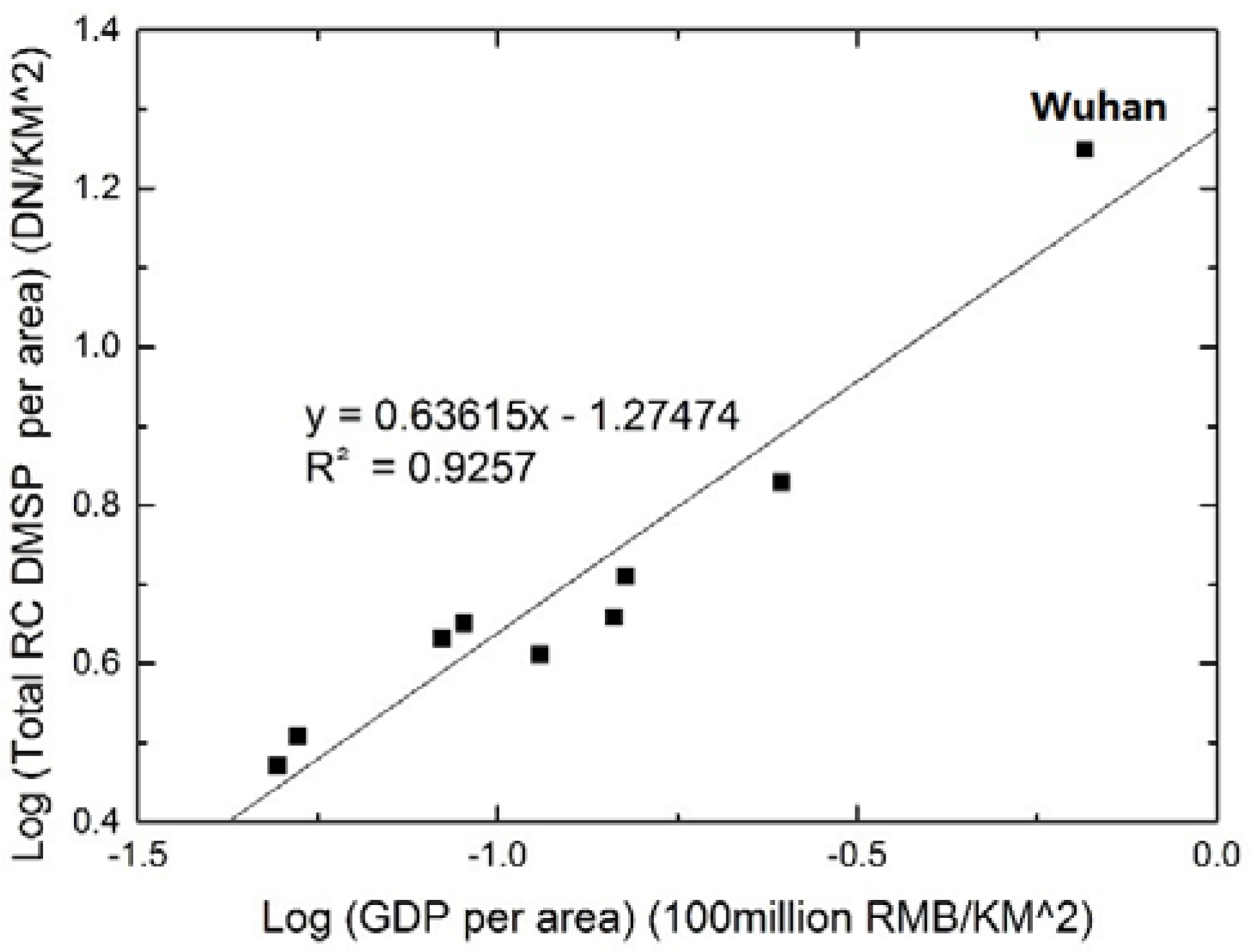
3.2. GDP Dasymetric Map

A dasymetric map of GDP can reveal the internal differences in a given region in terms of the level of economic development and provide a dataset for analyzing the spatiotemporal process of GDP growth. A number of methods have been used to estimate GDP using nighttime light data, such as linear regression models [21], log-log regression models [22], and second-order regression models [23]. A linear regression model is a relatively accurate and easy tool for estimating GDP using nighttime light data. Therefore, a linear regression model was established in each year at the prefectural level using DN values from the DMSP-OLS dataset as the independent variable

G_p = a × D_p + b

(3)

where G_p is statistical GDP data from each prefecture and D_p is the total DN value of DMSP-OLS data in the corresponding prefecture. Because a negative intercept b could lead to a negative GDP value at the grid level, the above empirical relationship was applied at the grid level as

G’_g = a × D_g

(4)

where G’_g and D_g are the estimated GDP value and DN value of DMSP-OLS data at the grid level (1 km), respectively. To correct the gridded GDP to best reflect the statistical GDP data from each prefecture, a normalization factor k was used to modify the estimated GDP at the grid level

G_g = k × G’_g,

(5)

k = G_p/∑_p × G’_g

where G_g is the final GDP value at the grid level, ∑_p G’_g is the total estimated GDP of each prefecture, and k is the normalization factor.

The original and corrected NRC data were used to estimate the spatial distribution of the GDP of the Wuhan urban agglomeration from 1992–2012. The regression results are shown in

Table 1. Regression models from 1992 to 2012 (GDP unit = 100 million RMB).

Year	NRC DMSP-OLS		Corrected DMSP-OLS
	Regression Model	R2	Regression Model	R2
1992	y = 0.0045x + 9.6097	0.9435	y = 0.0042x + 11.363	0.9630
1993	y = 0.0072x + 5.5751	0.9777	y = 0.0061x + 5.6131	0.9768
1994	y = 0.0100x − 2.6774	0.9775	y = 0.0084x − 2.6774	0.9775
1995	y = 0.0127x − 11.919	0.9764	y = 0.0123x − 11.952	0.9769
1996	y = 0.0153x − 22.355	0.9751	y = 0.0151x − 22.417	0.9757
1997	y = 0.0150x − 25.686	0.9817	y = 0.0128x − 21.877	0.9740
1998	y = 0.0169x − 29.908	0.9810	y = 0.0144x − 30.016	0.9818
1999	y = 0.0160x − 25.013	0.9834	y = 0.0122x − 25.143	0.9844
2000	y = 0.0180x − 48.724	0.9864	y = 0.0183x − 48.875	0.9873
2001	y = 0.0185x − 49.241	0.9921	y = 0.0168x − 49.412	0.9931
2002	y = 0.0206x − 85.218	0.9850	y = 0.0210x − 85.330	0.9855
2003	y = 0.0223x − 120.66	0.9726	y = 0.0148x − 120.73	0.9728
2004	y = 0.0237x − 155.38	0.9584	y = 0.0204x − 155.41	0.9585
2005	y = 0.0248x − 189.32	0.9440	y = 0.0215x − 189.33	0.9442
2006	y = 0.0257x − 222.50	0.9301	y = 0.0198x − 222.50	0.9301
2007	y = 0.0265x − 254.98	0.9170	y = 0.0246x − 254.96	0.9173
2008	y = 0.0289x − 293.35	0.9263	y = 0.0269x − 293.38	0.9263
2009	y = 0.0298x − 336.37	0.9380	y = 0.0180x − 336.37	0.9382
2010	y = 0.0368x − 317.45	0.9517	y = 0.0234x − 374.60	0.9404
2011	y = 0.0444x − 222.38	0.9543	y = 0.0228x − 400.22	0.9402
2012	y = 0.0377x − 464.73	0.9405	y = 0.0374x − 464.73	0.9405

at the prefectural level. Comparing NRC and corrected NRC data from 1992 to 2012, the latter exhibited higher determination coefficients (R²) than the former. This result indicated that corrected NRC data could be better used to create a dasymetric GDP map than could NRC data. However, the determination coefficient of correct NRC data was lower than that of non-corrected data in four years during the study period. This result occurred because the determination coefficients of the quadratic regression models used for intercalibration were lower in these four years, resulting in a large error associated with corrected NRC data after intercalibration.

Dasymetric GDP maps were produced using corrected NRC data from 1992 to 2012. Figure 4 shows the dasymetric GDP map in 2011. This map was estimated from corrected NRC data and prefectural level statistical data.

4. Map Spectrum-Based Spatiotemporal Clustering

With space–time trends, most studies have focused on the extraction of patterns in a spatial or temporal context [13]. This study proposed an improved k-means clustering method to extract these spatiotemporal patterns. Unlike the traditional k-means clustering method, in which clusters can only be formed in the space dimension or time dimension, the improved k-means algorithm can perform spatiotemporal clustering due to the proposed map spectrum representation model.

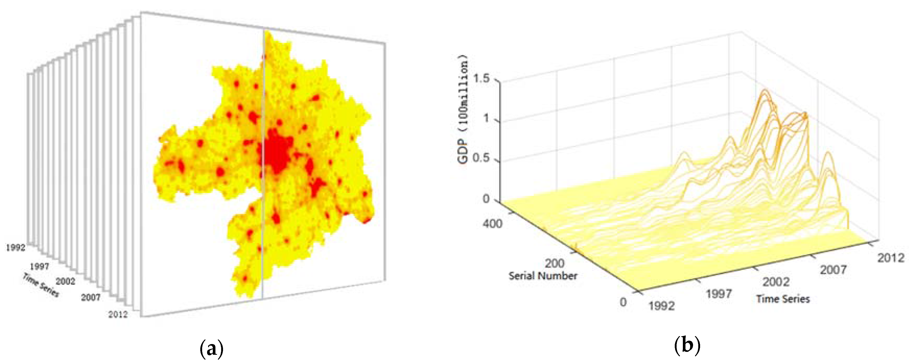
4.1. Map Spectrum-Based Spatiotemporal Representation Model

A spatiotemporally integrated representation model is crucial for spatiotemporal pattern extraction. Here, the spatial distribution of data was used to form a map. The distribution on the time axis is defined as the spectrum, and the map spectrum-based spatiotemporal representation model can be expressed as

MS = f(x, G(t))

(6)

where MS is the time spectrum of map, f (∙) is the spatiotemporal model, x is the spatial location of the grid unit, and G_x(∙) is the value of the data within unit x at time t. For effective visualization, GDP distributions of one-column pixels (Figure 5a) from 1992 to 2012 are used as samples to generate a spatiotemporal map spectrum (Figure 5b) based on the model shown in Equation (6). To obtain the GDP trend, min–max normalization was performed for each pixel in the GDP time spectrum. In Figure 5b, the axis labeled “serial number” represents the position of the pixel in the image, and the GDP spectrum represents the normalized GDP value in each year at the same location.

4.2. Similarity Measurement of the Map Spectrum Model

The similarity measurement between spectrum lines is the key component of the map spectrum-based spatiotemporal clustering model. In this study, the cosine of two vectors consists of node variables of the spectrum line, as shown in Equation (7)

$$\cos \varnothing =\frac{{{\displaystyle \sum }}_1^n\left(a_i\times b_i\right)}{\sqrt{{{\displaystyle \sum }}_1^n{a}_i^2}\times \sqrt{{{\displaystyle \sum }}_1^n{b}_i^2}}$$

(7)

where vectors $a=\left\{a_1,a_2,a_3,\cdots ,a_n\right\}$ and $b=\left\{b_1,b_2,b_3,\cdots ,b_n\right\}$ represent nodes of spectrum lines that are involved in similarity measurements. The range of the cosine value between two vectors is [0,1]. The close the value is to 1, the higher the similarity of the two spectrum lines.

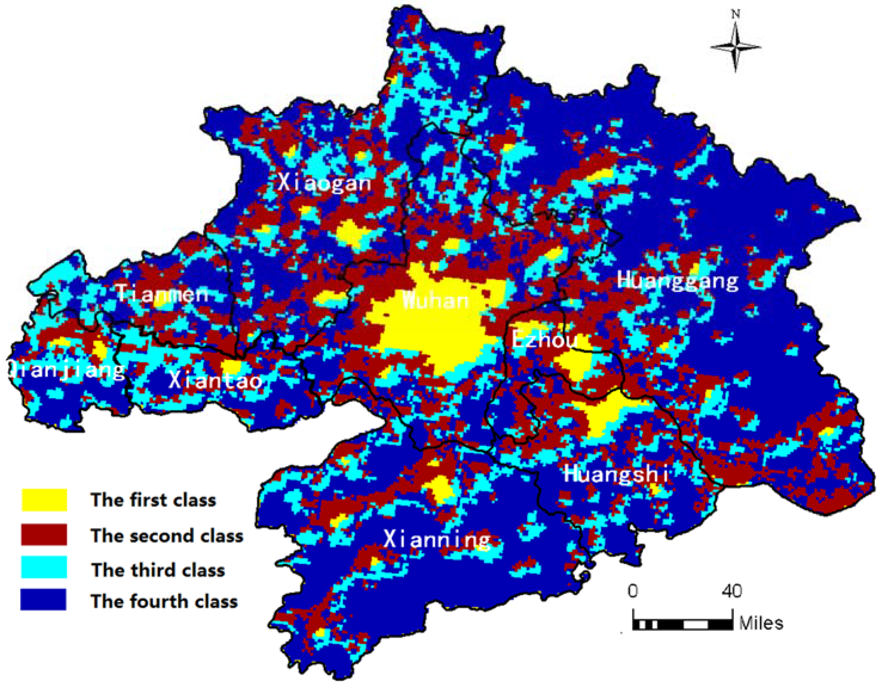
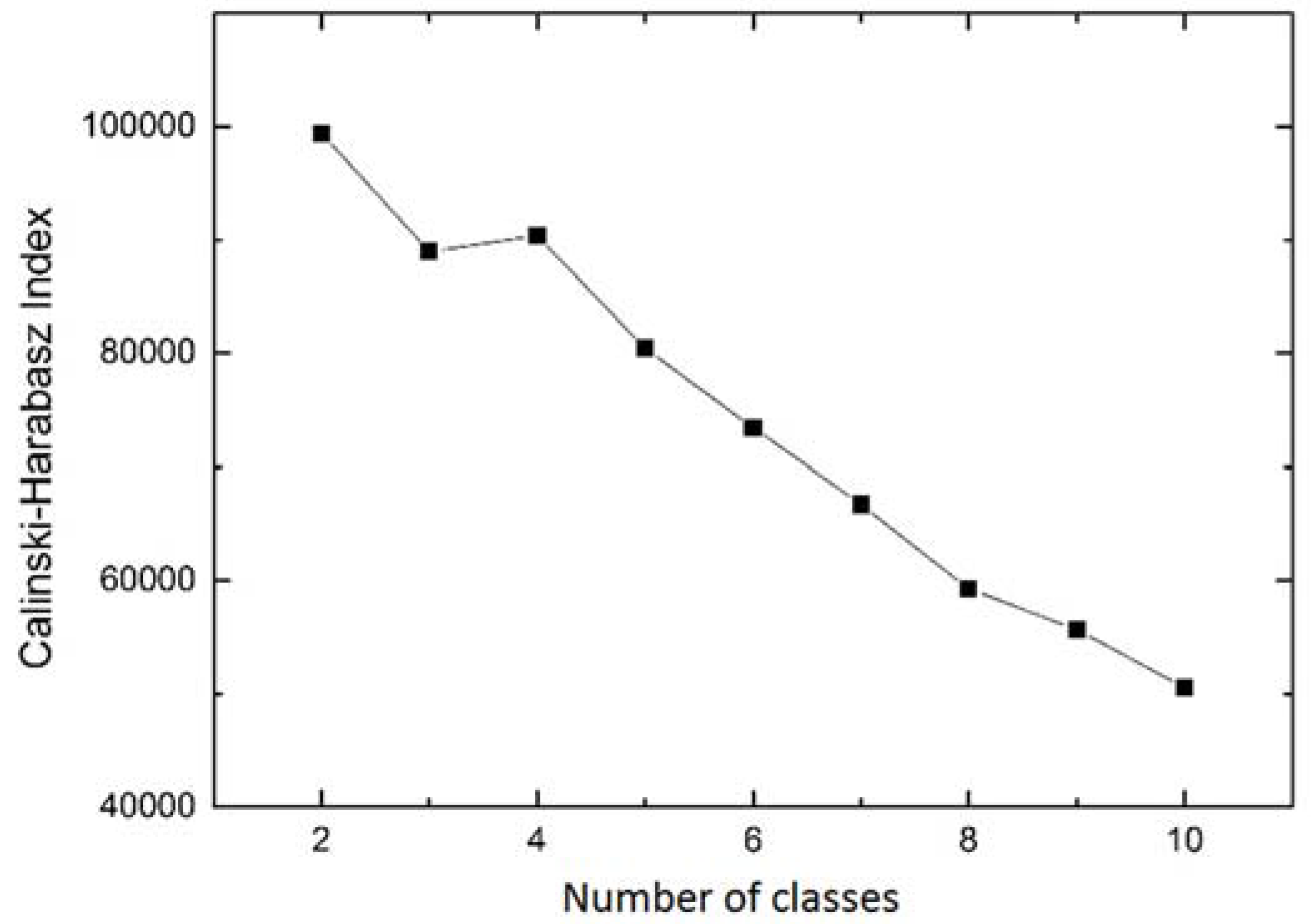
4.3. Extraction of Spatiotemporal Patterns

Previous studies have shown that the k-means clustering method can produce stable cluster boundaries based on a spatial sensitivity analysis test [7]. Thus, the improved k-means clustering method was applied to dasymetric GDP maps of the Wuhan urban agglomeration from 1992 to 2012 to obtain patterns in spatiotemporal variations.

Two major factors must be considered to obtain a reasonable clustering result. First, a set of random initial mean centers must be allocated. To reduce the dependence of the results on the initial allocation of mean centers, the initial mean centers were uniformly selected at random from the range of all values of similarity and were iterated 10 times to generate the clustering result. Second, the number of classes must be determined. The Calinski–Harabaz index [24] can be used to evaluate this number when actual values are unknown. Given a clustering approach with a certain number of classes, the Calinski–Harabaz score is defined as the ratio of the between-cluster dispersion to the within-cluster dispersion. A high Calinski–Harabaz score indicates that clusters are well separated and defined. In Figure 6, the Calinski–Harabaz index of two-class clustering exhibited the highest score. However, two classes are not sufficient for differentiating between GDP variations because one of the classes represents areas of no night light. Therefore, we chose four-class clustering, which had the second highest score, as the number of classes sufficiently represented patterns in GDP variations.

According to the Calinski–Harabaz scores, the spatiotemporal variations in GDP were clustered into four classes. The clustering results are shown in Figure 7. The fourth class, which represented areas with no night lighting, cannot reflect the spatiotemporal variations in GDP; thus, the first three classes were used to analyze the variation pattern.

5. Discussion

5.1. Accuracy Assessment of the Dasymetric GDP Map based on County-Level GDP Statistics

The administrative units of mainland China contain five levels: the province, prefecture, county, township, and village levels. In Section 3.2, prefecture-level GDP data were used to produce dasymetric GDP maps. Therefore, county-level GDP data were used to validate dasymetric GDP maps. We collected statistical GDP data from 13 districts/counties in Wuhan from 1997 to 2012 and calculated the total GDP value of each district/county from the corresponding dasymetric GDP map based on the county boundary. Three statistical measures—namely, the root mean square error (RMSE), mean relative error (MRE), and correlation coefficient (R)—were used to assess the accuracies of dasymetric GDP maps.

Table 2. Three statistical measures based on estimated and actual GDP in the 13 districts/counties of Wuhan (GDP unit = 100 million RMB).

Year	RMSE	MRE	R
1997	4.9614	4.5572%	0.9982
1998	3.6867	3.0326%	0.9992
1999	1.8850	1.8516%	0.9988
2000	4.2335	3.3435%	0.9949
2001	3.2224	2.5797%	0.9989
2002	3.3361	2.1376%	0.9995
2003	10.9458	6.1353%	0.9729
2004	8.1877	4.0032%	0.9895
2005	28.8478	11.4043%	0.9649
2006	14.3577	5.1784%	0.9929
2007	22.5479	7.4647%	0.9826
2008	17.6268	4.3592%	0.9934
2009	12.5426	2.8741%	0.9969
2010	19.7350	3.8184%	0.9935
2011	48.0933	7.6910%	0.9694
2012	68.3982	9.3377%	0.9468

shows the validation results of the estimated GDP for 13 districts/counties in Wuhan. From 1997 to 2012, the RMSE increased due to the nearly 10-fold growth in the Wuhan GDP. The high R and low MRE values in each year indicated that the estimated and actual GDP values were similar at the county level. The validation results suggested that nighttime light data could be effectively used to create dasymetric GDP maps of the Wuhan urban agglomeration, and the estimated dasymetric maps accurately expressed the spatial distribution of the GDP.

5.2. GDP Variation Pattern Analysis based on the Clustering Results

Based on Chinese land use/cover datasets from 1995, 2000, 2005, and 2010, three land use types—including urban built-up area, rural residential area, and industrial area—were counted for each clustering class. Figure 8 illustrates the statistical results of the three land use types for each class. A comparison of Figure 8a–c indicates that the main land use type in the first class is urban built-up area, which suggests that the first class is associated with urban centers in large, medium, and small cities. The main land use type of the second and third classes is rural residential area. However, urban built-up area is much more common in the second class than in the third class. Therefore, the second class is generally associated with urban fringe areas, and the third class is associated with areas in the countryside.

Figure 9 shows the GDP variations in the above three classes over time. In Figure 9, the x-axis categories represent the clustering classes, and the GDP variations represent the change in the average GDP of each class in two adjacent years. The overall GDP variation in the study area was relatively minor before 2007, and rapid growth occurred after that point. The cause of this growth was the approval of the Wuhan Metropolitan Area as a reform area with a resource-conserving and environmentally friendly society in 2007. The establishment of reform policy promoted economic connection and integration between the cities in the study area.

Differences in the GDP variation pattern of each class can be observed from 1992 to 2012. The GDP variations of the first class, representing urban centers, fluctuated considerably. Before 2007, because the government took the lead in developing the economy in eastern coastal areas, urban economic development in the study area slowed and even regressed. At that time, due to policy impacts, many resource-intensive industries relocated, which caused the GDP to briefly decline. Since then, with the development of urbanization and tertiary industry growth, GDP growth has significantly accelerated. The second class represents the GDP change in urban fringe areas. Before 2007, the GDP variations in these regions were small because these undeveloped areas were dominated by primary industry. Then, with the acceleration of urbanization and industrial structure transformation caused by industry migration, secondary and tertiary industries became active in these areas and led to rapid GDP growth. The GDP development of the third class was stagnant because these areas are distributed in rural areas. The small GDP increase in these areas was associated with the radiation effect of GDP growth in the Wuhan Metropolitan Area. Moreover, due to the continuous development of agricultural production technology, the GDP increased in areas engaged in primary industry.

6. Conclusions

The dasymetric map of GDP is an important means of reflecting the spatial differences in GDP within an administrative unit. In addition, the spatiotemporal pattern of GDP is generally used to measure the growth characteristics of the GDP of a region or country. Thus, these results provide an important basis for economic development and planning as well as precise decision making during economic management. The main contributions of this study can be summarized as follows:

(1)

This study investigated the mapping of statistical GDP data based on spatial location to obtain a dasymetric GDP map using DNs from calibrated night light images. A linear regression model between DN and GDP was constructed at a prefectural level, and normalization factors between grid-level GDP and prefectural GDP statistics were used to produce accurate dasymetric GDP maps.

(2)

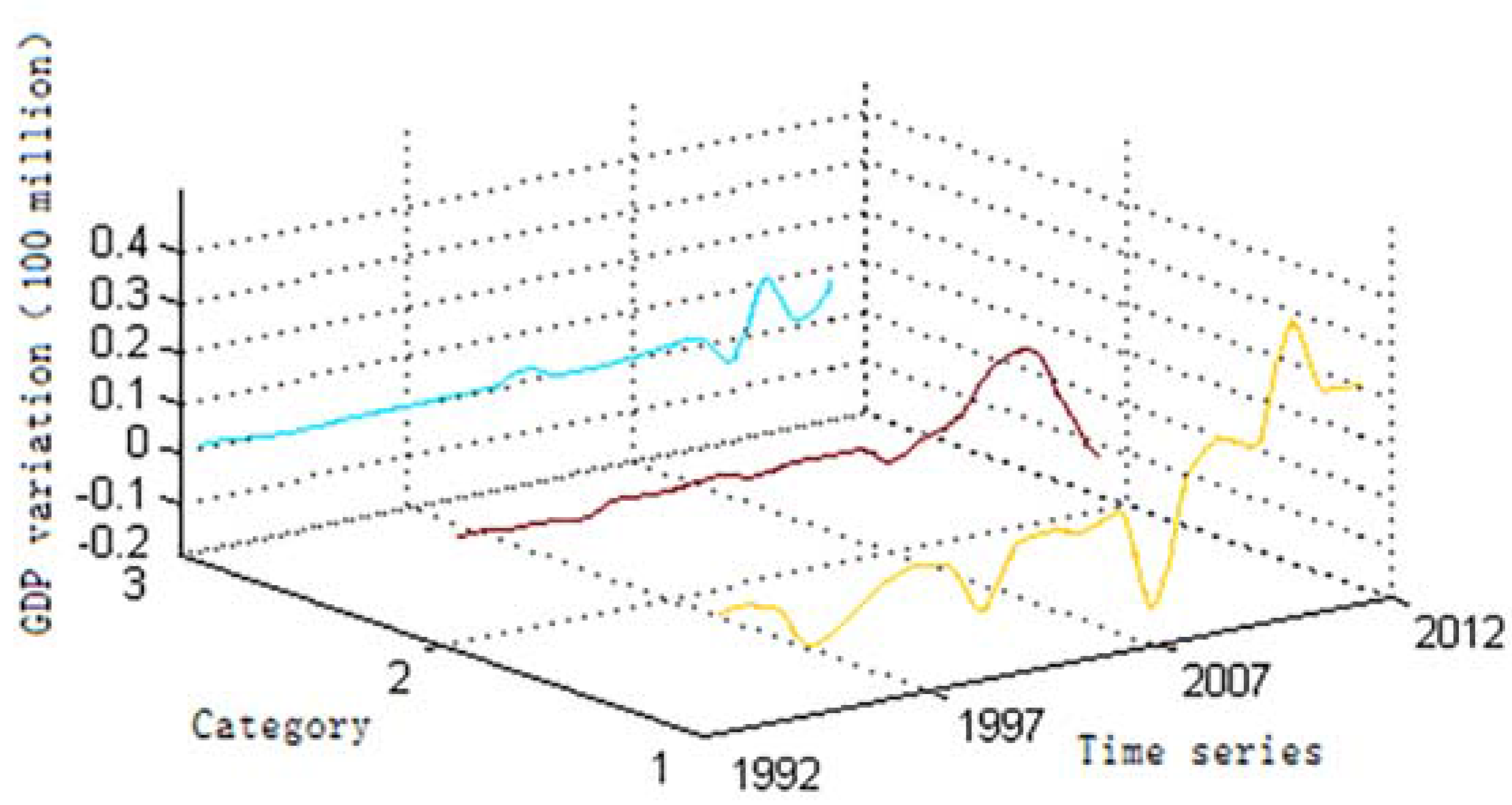
To investigate GDP growth, this study proposed a method of improved k-means clustering using a map spectrum-based, spatiotemporally integrated model. The proposed spatiotemporal representation model is a 3D model consisting of time, space, and magnitude dimensions. The model provides a solution that simultaneously considers spatial and temporal characteristics in clustering.

(3)

This study produced dasymetric maps and obtained the spatiotemporal patterns of GDP growth in the Wuhan urban agglomeration. These findings provide an important basis for economic development, spatial planning, decision making, and management in the region. In addition, the study provides a reference solution for spatial mapping and spatiotemporal pattern extraction using other socioeconomic data.

References

1. Zeng, C.Q.; Zhou, Y.; Wang, S.X.; Yan, F.L.; Zhao, Q. Population spatialization in China based on night-time imagery and land use data. Int. J. Remote Sens. 2011, 32, 9599–9620. [Google Scholar] [CrossRef]
2. Lopes, F.B.; da Silva, M.C.; Miyagi, E.S.; Fioravanti, M.C.S.; Faco, O.; Guimaraes, R.F.; Junior, O.A.D.; McManus, C.M. Spatialization of climate, physical and socioeconomic factors that affect the dairy goat production in Brazil and their impact on animal breeding decisions. Pesqui. Vet. Bras. 2012, 32, 1073–1081. [Google Scholar] [CrossRef]
3. Cao, X.; Wang, J.M.; Chen, J.; Shi, F. Spatialization of electricity consumption of China using saturation-corrected DMSP-OLS data. Int. J. Appl. Earth Obs. Geoinform. 2014, 28, 193–200. [Google Scholar] [CrossRef]
4. Silva, C.S.P.; Grigio, A.M.; Pimenta, M.R.C. Survey and spatialization crime urban county Mossoro-Rn. Holos 2016, 32, 352–362. [Google Scholar] [CrossRef]
5. Talebi, M.; Zare, M.; Madahi-Zadeh, R.; Bali-Lashak, A. Spatial-temporal analysis of seismicity before the 2012 Varzeghan, Iran, Mw 6.5 earthquake. Turk. J. Earth Sci. 2015, 24, 289–301. [Google Scholar] [CrossRef]
6. Wang, Z.Y.; Ye, X.Y.; Tsou, M.H. Spatial, temporal, and content analysis of twitter for wildfire hazards. Nat. Hazards 2016, 83, 523–540. [Google Scholar] [CrossRef]
7. Zhang, Y.; Moges, S.; Block, P. Optimal cluster analysis for objective regionalization of seasonal precipitation in regions of high spatial-temporal variability: Application to western Ethiopia. J. Clim. 2016, 29, 3697–3717. [Google Scholar] [CrossRef]
8. Vogel, C.R.; Tyler, G.A.; Wittich, D.J. Spatial-temporal-covariance-based modeling, analysis, and simulation of aero-optics wavefront aberrations. J. Opt. Soc. Am. a-Opt. Image Sci. Vis. 2014, 31, 1666–1679. [Google Scholar] [CrossRef] [PubMed]
9. Qian, T.N.; Bagan, H.; Kinoshita, T.; Yamagata, Y. Spatial-temporal analyses of surface coal mining dominated land degradation in Holingol, Inner Mongolia. IEEE J. Sel. Top. Appl. Earth Obs. Remote Sens. 2014, 7, 1675–1687. [Google Scholar] [CrossRef]
10. Li, X.; Li, D.R. Can night-time light images play a role in evaluating the Syrian crisis? Int. J. Remote Sens. 2014, 35, 6648–6661. [Google Scholar] [CrossRef]
11. McArdle, G.; Tahir, A.; Bertolotto, M. Interpreting map usage patterns using geovisual analytics and spatio-temporal clustering. Int. J. Digit. Earth 2015, 8, 599–622. [Google Scholar] [CrossRef]
12. Chidean, M.I.; Munoz-Bulnes, J.; Ramiro-Bargueno, J.; Caamano, A.J.; Salcedo-Sanz, S. Spatio-temporal trend analysis of air temperature in Europe and western Asia using data-coupled clustering. Glob. Planet. Chang. 2015, 129, 45–55. [Google Scholar] [CrossRef]
13. Wu, X.J.; Zurita-Milla, R.; Kraak, M.J. Co-clustering geo-referenced time series: Exploring spatio-temporal patterns in Dutch temperature data. Int. J. Geogr. Inf. Sci. 2015, 29, 624–642. [Google Scholar] [CrossRef]
14. Damiani, M.L.; Issa, H.; Fotino, G.; Heurich, M.; Cagnacci, F. Introducing ‘presence’ and ‘stationarity index’ to study partial migration patterns: An application of a spatio-temporal clustering technique. Int. J. Geogr. Inf. Sci. 2016, 30, 907–928. [Google Scholar] [CrossRef]
15. NOAA. Available online: http://ngdc.noaa.gov/eog /download.html (accessed on 24 March 2017).
16. RESDC. Available online: http://www.resdc.cn (accessed on 24 March 2017).
17. Liu, Z.F.; He, C.Y.; Zhang, Q.F.; Huang, Q.X.; Yang, Y. Extracting the dynamics of urban expansion in China using DMSP-OLS nighttime light data from 1992 to 2008. Landsc. Urban Plan. 2012, 106, 62–72. [Google Scholar] [CrossRef]
18. Lo, C.P. Urban indicators of China from radiance-calibrated digital DMSP-OLS nighttime images. Ann. Assoc. Am. Geogr. 2002, 92, 225–240. [Google Scholar] [CrossRef]
19. Elvidge, C.D.; Ziskin, D.; Baugh, K.E.; Tuttle, B.T.; Ghosh, T.; Pack, D.W.; Erwin, E.H.; Zhizhin, M. A fifteen year record of global natural gas flaring derived from satellite data. Energies 2009, 2, 595–622. [Google Scholar] [CrossRef]
20. Liu, J.; Li, W. A nighttime light imagery estimation of ethnic disparity in economic well-being in mainland China and Taiwan (2001–2013). Eurasian Geogr. Econ. 2015, 55, 691–714. [Google Scholar] [CrossRef]
21. Shi, K.F.; Yu, B.L.; Huang, Y.X.; Hu, Y.J.; Yin, B.; Chen, Z.Q.; Chen, L.J.; Wu, J.P. Evaluating the ability of NPP-VIIRS nighttime light data to estimate the Gross Domestic Product and the Electric Power Consumption of China at multiple scales: A comparison with DMSP-OLS data. Remote Sens. 2014, 6, 1705–1724. [Google Scholar] [CrossRef]
22. Lo, C.P. Modeling the population of china using DMSP operational linescan system nighttime data. Photogramm. Eng. Remote Sens. 2001, 67, 1037–1047. [Google Scholar]
23. Wu, J.S.; Wang, Z.; Li, W.F.; Peng, J. Exploring factors affecting the relationship between light consumption and GDP based on DMSP/OLS nighttime satellite imagery. Remote Sens. Environ. 2013, 134, 111–119. [Google Scholar] [CrossRef]
24. Calinski, T.; Harabasz, J. A dendrite method for cluster analysis. Commun. Stat. 1974, 3, 1–27. [Google Scholar] [CrossRef]
Figure 1. Study area.
Ijgi 06 00160 g001
Figure 2. Relationship between GDP per km2 and total RC DMSP-OLS per km2 in 2011.
Ijgi 06 00160 g002
Figure 3. Sum of DNs in the study area from 1992 to 2012 across all nighttime light satellite missions: (a) before calibration and (b) after calibration. F10, F12, F14, F15, F16, and F18 are the six nighttime light satellite missions in the dataset.
Ijgi 06 00160 g003
Figure 4. Dasymetric GDP map in 2011.
Ijgi 06 00160 g004
Figure 5. Time Spectrum of GDP maps for given column pixels from 1992 to 2012. (a) Position of the column that was used to generate the spatiotemporal map spectrum. (b) Time Spectrum.
Ijgi 06 00160 g005
Figure 6. Calinski–Harabaz score for different numbers of classes.
Ijgi 06 00160 g006
Figure 7. Results of spatiotemporal clustering based on four classes.
Ijgi 06 00160 g007
Figure 8. The statistical results of three land use types for three clustering classes in four years: (a) The first class; (b) The second class; (c) The third class.
Ijgi 06 00160 g008
Figure 9. Time-varying patterns of the three classes.
Ijgi 06 00160 g009