Spatial Dynamic Modelling of Future Scenarios of Land Use Change in Vaud and Valais, Western Switzerland

Abstract

We use Bayesian methods with a weights of evidence approach to model the probability of land use change over the Western part of Switzerland. This first model is followed by a cellular automata model for spatial allocation of land use classes. Our results extend and enhance current land use scenarios studies by applying Dinamica Environment for Geoprocessing Objects (Dinamica EG) to a study area comprising of the upper Rhone river basin in the Cantons of Vaud and Valais. In order to take into account the topography, we divide the study area into four regions, based on their altitude and administrative region. We show that the different regions are affected in differing ways by the same driving forces. We analyse possible outcomes in land use change in 2050 for three different scenarios: “business as usual”, “liberalisation” and a “lowered agriculture production”. The “business-as-usual” scenario results indicate a decrease in agriculture, mostly in extensive agriculture, with a share in the total area of 12.3% in 2009 decreasing by 3.3% in 2050. Losses expected under a “business-as-usual” scenario in agriculture, are mostly due to the conversion to shrubland and forest. Further losses in extensive agriculture are expected under the “liberalisation” scenario, decreasing by 10.3 % in 2050. Along with a marked increase in the closed and open forest area, increasing from 27.1% in 2009 to 42.3% by 2050. Gains in open land habitat with the increase of the share of extensive agriculture area under the “lowered agricultural production” scenario are expected to increase by 3.2% in 2050, while the share of intensive agriculture area is expected to decrease by 5.6%.

1. Introduction

The land use/cover change field of research is equally concerned with modelling changes, as well as creating plausible scenarios, and has been broadly discussed and recognized in the context of global and regional change [1,2,3,4,5]. In general, different studies have demonstrated the importance of understanding and modelling the land use/cover change, to assess soil erosion and instability [6,7], to estimate carbon emissions from deforestation and forest degradation [8,9], to model water quality and quantity [10,11,12], to predict species habitat [13,14,15] , and on the intensity and size of wildfires [16].

Scenarios of land use/land cover change offer the possibility to project current and alternative future changes and, thus, allowing the mitigation of potential impacts and improve planning [2,5]. They try to replicate the behaviour of past land use/land cover by considering not only the environmental suitability of the land to support specific land use/cover categories, but social and economic driving forces as well [2,3,17,18,19,20]. The environmental, social, and economic driving forces for each land use/cover cell and their neighbourhood influence are considered by the model [6,8,21,22], and are implemented, for example, by means of a cellular automaton (CA) [8,23]. The CA is a spatially explicit dynamic system method with a simple structure: the main component is a collection of cells arranged in an evenly spaced grid (representing the current land use/cover dataset), where each cell is characterized by a suitability defined from the driving forces, representing the capacity of a cell to support a particular activity (in this case a land use type); transition rules, their neighbourhood influence and the time frame. At each time step the shape formed by a group of land use/cover cells evolves according to the defined transition rules, geometry, as well as the neighbourhood influence, and can, additionally, incorporate a random variable to allow for some unpredictability [8]. As such, the CA model is a valuable tool for modelling scenarios [9,24,25].

In Switzerland there is a paucity of information concerning future scenarios [13,17,26]. Existing European regional projects for the analysis and projection of scenarios either do not cover Switzerland (Eururalis [5]) or only cover the country to a small degree (enviroGRIDS [2]). The available studies consider only few transitions in the landscape [13,25,27] and focus on specific topics, such as forest change [28,29,30], agriculture abandonment and forest regrowth [31], urban growth [32,33], mountainous landscape [34], and implications of land use/cover change in the species habitat [13]. Modelling multiple transitions becomes complex. Rutherford et al. [34] evaluated different sampling and logistic regression methods for the full Swiss territory using four different land use change categories. Only one study applies spatial dynamic modelling [26], however changes in glaciers are not taken into consideration in the model. Existent studies suggest difficulties in modelling land use/cover change for the full Swiss territory [34], while, for the administrative regional level the modelling and allocation is considered suitable [34].

The main aim of this study is to improve the existent land use scenarios for the upper Rhone river basin in the mountainous region of Switzerland covering the Cantons of Vaud and Valais from 2009 to 2050. We use Dinamica Environment for Geoprocessing Objects (Dinamica EGO) [23,35], a modelling approach not yet applied to this area. In this context, the current research has the following objectives: (a) to identify and discuss the main driving forces of land use change; (b) model multiple land use transitions, glaciers; and (c) discuss the impact of different economic scenarios that were studied in: a “business-as-usual” scenario, which relies on trends of change observed in the past; a “liberalization scenario”; and a “lowered agriculture production” scenario [13].

This paper is organized as follows. We start by describing the study area the datasets in Section 2 and Section 3. A synthesis of the modelling approach is developed in Section 4. Scenarios of land use change are explored in Section 5. In Section 6, we provide a summary of the most relevant results for the calibration and scenarios. Section 7 provides a discussion of the results and identifies key improvements to the model.

2. Study Area

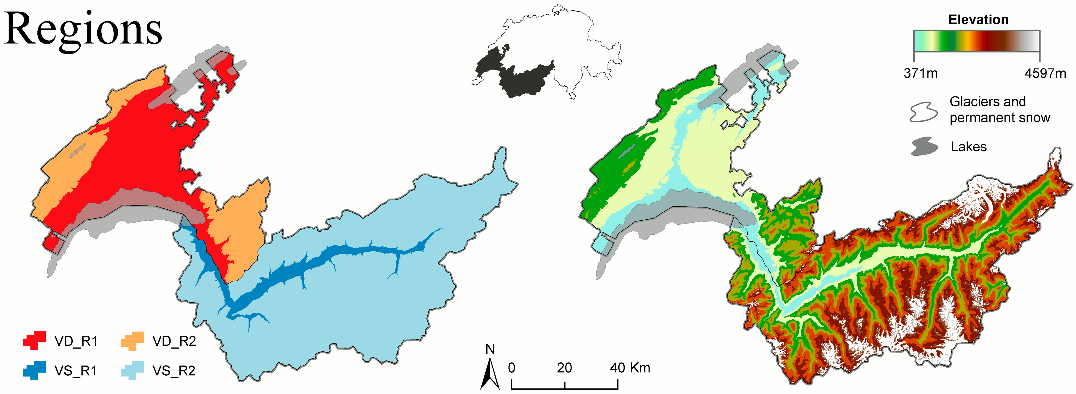
The study area the cantons of Vaud and Valais (Figure 1) in Western Switzerland. These two cantons were chosen based on their contrasting topography, and climatic and economic conditions. The Valais is located in the southwest, covering an area of 5224 km², and includes the upper part of the Rhone basin with altitudes varying between 372 and 4634 m above sea level (m a.s.l.). It is a highly glaciated region with the glaciers being the principal source of water for the Rhone river. The area is comprised 47% of unproductive land, 30% of which is glaciers and permanent snow. The climate is considered cold and dry [36]. Above 900 msal, the mean monthly cumulative precipitation between 1961 and 1990 was 1007.2 mm/month and the mean temperature was 2.1 °C [36]. Bellow 900 m a.s.l., the mean monthly cumulative precipitation was 683.4 mm/month and the mean temperature was 8.9 °C [36]. The canton of Vaud stretches from the canton of Valais to the North and West, covering an area of 3212 km². Vaud is also a mountainous area with principal mountain regions being the pre-Alps in the south (north of the Rhone) and the Jura in the north. These areas are linked by a plateau with altitudes varying between 370 m a.s.l. at the shores of Lac Léman to 3180 m a.s.l. Vaud has a lower percentage of mountainous territory than the Valais. Agriculture (intensive and extensive) and industry land uses occupy 40% and 13% of the canton’s surface, respectively. The climate in this region is considered to be temperate and highly influenced by the lakes Léman and Neuchâtel [36]. Above 900 m a.s.l., the mean monthly cumulative precipitation between 1961 and 1990 was 1648.0 mm/month and the mean temperature was 4.6 °C [36]. Bellow 900 m a.s.l., the mean monthly cumulative precipitation was 1093.6 mm/month and the mean temperature was 9.5 °C [36]. The results obtained in a recent study suggests that modelling the land use changes in Switzerland at a regional level would be more reliable [34]. In order to create more reliable land use change model, we divide the study area into multiple regions where each region can be modelled with different driving forces and individual change demand. Following the work carried out previously [13], we divided the study area into two elevation bands (below and above 900 m a.s.l.); in addition, we subdivided each elevation band by administrative region.

3. Land Use and Drivers of Land Use Change

The land use (LU) datasets used in this study were obtained from the Swiss Federal Statistics Office (SFSO) and are comprised of three sequential datasets for the periods 1979 to 1985, 1992 to 1997, and 2004 to 2009, with a spatial resolution of 100 m. The last year of the three sequential datasets was taken as the reference year and the datasets are designated as 1985, 1997, and 2009. The land use nomenclature used by the SFSO was selected with the aim of efficiently retaining both land use and land cover, according to the observation made in six regions [37]. For this study the original categories were aggregated into 14 classes, as shown in

Table 1. Original Swiss land use classes and new aggregated classes. * Classes that were not modelled and, thus, considered static.

Aggregated Class	Swiss Land Use Classes (1995/97, 2009)
1 closed forest	Forest fresh cuts; Other forest; Normal dense forest; Forest stripes, edges; Brush forest
2 open forest	Open forest (on unproductive areas); Open forest (on agriculture areas); Groves, hedges; Clusters of trees (on agriculture areas); Other woods
3 permanent crops	Horticulture; Intensive orchards; Extensive orchards; Scattered fruit trees; Regular vineyards; ‘Pergola’ vineyards; Extensive vineyards
4 intensive agriculture	Favourable arable land and meadows; Other arable land and meadows; Natural pastures
5 extensive agriculture	Farm pastures; Mountain meadows; Favourable alpine pastures; Rocky alpine pastures; Remote and steep alpine meadows and pastures
6 shrubland	Scrub vegetation; Brush meadows and farm pastures; Brush alpine pastures; Unproductive grass and shrubs; Alpine sports infrastructure
7 open spaces with little or no vegetation *	Roads; Dams; Avalanches protection; Construction sites
8 urban	Urban buildings; Land around urban buildings
9 industry	Industrial buildings; Land around industrial buildings
10 mine, dump, construction sites and transport units *	Ruins, Energy and waste plants; Transport network
11 glaciers and permanent snow	Glacier and permanent snow
12 urban parks *	Green spaces
13 rocks and sand *	Bare rock and sand
14 inland waters and wetlands *	Lakes; Rivers; River shores; Wetlands; Shore vegetation

. The “glaciers and permanent snow” land use category was not used by the SFSO in the 1985 dataset and, for this reason, only the 1997 and 2009 datasets were selected to calibrate the model.

The drivers of land use change were chosen based on previous studies [17,23,34,38]. For this study, local factors, such as climate, topography, distance variables, and agriculture regions, were used as drivers of land use change. Drivers of land use change are summarized in

Table 2. Drivers of land use change.

Name	Description	Units	Source
ELEVATION	Height above sea level	m	Derived from SWISSTOPO (DEM25)
SLOPE	Slope angle	degree of slope
TOPO	Topographic position index (25 m)	-
TWI25	Topographic wetness index (25 m)	-
TRI	Terrain roughness index (25 m)	-
TEMP	Mean annual temperature (1961–1990)	1/100 °C	WSL Zimmermann and Kienast (1999)
PCP	Mean annual precipitation (1961–1990)	1/10 mm
SWB	Site water balance (1961–1990)	(1/10 mm)/year
MSRAD	Mean annual solar radiation calculated on the basis of monthly values	KWH/m2
MMIND	Mean annual moisture index calculated on the basis of monthly index	index
GAMS	Continentality Index	index
APTSOIL	Soil potential for agriculture extracted from the Swiss soil suitability map	-	AGROSCOPE
LIMAGRIC	Agriculture regions	-	OFS
POP	Habitation buildings density by 2 ha (1990–2000) Census	-
DistPerturb	Distance to landscape disturbance	m
DensityRoad	Density of roads by 1 ha	-	Derived from SWISSTOPO (DEM25)
DistAA	Euclidean distance to highways accesses	m
DistHydro	Euclidean distance to rivers and lakes	m

. In addition we use the multiscale analysis of the terrain rugosity (terrain roughness index) [39], density of habitation buildings within a neighbourhood of 2 ha, obtained from the 1990 and 2000 census , the Euclidean distance from lakes and rivers, and road density (within 1 ha). In addition, the dynamic distances to the transition outcome are calculated automatically for each time step by Dinamica EGO. Distance from observed changes in the landscape as well as the Euclidean distances from highway accesses, were also used as variables of land use change in Vaud and Valais below 900 m a.s.l.. Furthermore, the agriculture zones defined by the Federal Office for Agriculture [40] that are subject to financial support from the government were also used.

4. Modelling Approach

We use Dinamica EGO (Version 2.2.6) with statistical inference and a Cellular Automata allocation algorithm. Dinamica EGO requires the creation of one model that will be used in both calibration and simulation. The land use/cover change simulation in Dinamica EGO can be divided into a series of distinct steps: estimation of the annual transition rates for each land use change, quantification of land transition probability based on the WoE method, spatial allocation of land use changes, calibration, and validation. Figure 2 illustrates the workflow process for land use/cover change modelling with Dinamica EGO.

The first step in the model calibration is the estimation of the annual transition rates, obtained by the calculation of a cross-tabulation between the two land use datasets, resulting in the percentage change for each land use transition to be applied for each time step [8]. The total of 100 cells (100 ha) was estimated as the minimum change needed to obtain an accurate correlation and causation between change and driving forces; therefore, transitions with less than 100 cells were not modelled.

Then, the spatial probability of land use change occurrence based on a set of driving forces is obtained by the weight of evidence (WoE) method. The WoE is a statistical inference method, that applies claims of risk that result from interpretative methods of risk assessment [38] to estimate the transition potential, based on a set of “evidence” variables. Applied to land use change, the method calculates the weight for each land use driver based on the presence or absence of each land use change. WoE only applies to categorical data. Consequently, the drivers of land use change must be transformed from continuous image data to categorized image data. This transformation is done with a method first developed by Agterberg and Bohan Carter (1990) (cited in [23]) and adapted by [23], preserving the data structure of the imagery. The WoE method has been used as a replacement for descriptive static methods, like logistic regression. The two methods differ in the way the relationship between the probability of land use change and the drivers is modelled. The logistic regression assumes that the relationship between the land use change and the drivers is a logistic function, however, this relationship has been proven to be too generalist [41,42,43], while the WoE is more flexibility in modelling the relationship between the probability of change and the drivers, which is calculated independently [8]. For this reason all driving forces must be spatially independent. A set of correlation tests measuring Cramer’s coefficients, contingency coefficient, and joint information uncertainty can be applied to assess the existence of spatial correlation (for a full description of the methodology see [23]). The WoE method assigns weights for each land use driver category [44]. A positive weight indicates that a certain range of values is present at the land use change locations and the magnitude of this weight is an indication of the positive correlation between the presence of the range of values and the land use change. A negative weight indicates the absence of land use change and shows the level of negative correlation. The difference between the two weights is known as the weight contrast, and is a measurement of the spatial association or relation for each land use change [44]. The spatial probability for each land use change is then obtained by summing up the WoE of each driving force. Dynamic drivers of land use change can be added to the WoE, such as distance to a specific land use type. For each time-step the dynamic distances are updated, the WoE is calculated and the spatial probability updated.

The land use changes are then allocated using a cellular automata model, where each land use cell changes between categories according to the annual transition rates, their spatial probability (WoE), and transitions rules [23]. The implementation of the transition rules is made by means of two complementary rules: Expander and Patcher.

They divide the behaviour of the observed change of a certain type of land use, into expansion or regression of existing groups of land use cells (patches), and the creation of new independent patches [23]. These rules evolve for a number of time steps specified by the user for each land use category. First the Expander rule is applied, allowing both the expansion as well as the contraction, of previous patches to their nearest neighbour cells [9,21]. The remaining cells are then allocated to new independent patches using the Patcher rule. The proportion of the change demand that is allocated by the Expander rule and transferred to the Patcher rule is defined by the user [23]. In this study the estimation of the amount of land use change to be allocated by both rules was performed using a custom landscape change analysis script created using the ArcPy Python library. First a cross-tabulation raster between the initial and the final land use maps is calculated for each land use transition, followed by the calculation of the total number of cells in new patches and the number of cells in newly-created patches that share a line segment with previous existing land use patches. The later percentage is attributed to the Expander rule, and the remaining to the Patcher rule. In each time step, for each land use change, both rules first arrange cells with the highest spatial probability of change (obtained with the WoE method) in a data array and then selects transition cells from the top to the bottom of the array to be allocated. The length of the array is determined by the annual transition rates and the percentage attributed to the rule. The control of the geometry the land use patches is made by estimating their mean, standard deviation, and isometry [23]. Both mean and standard deviation values are not applied directly to create new patches, but to define a lognormal probability distribution. From the lognormal probability distribution random values for both mean and standard deviation are then extracted and applied to create new patches [8,23]. The geometry analysis was made using the Species Distribution Modelling Tools (SDMTools) [33] in R. The outputs from the landscape change analysis script were loaded into R and the ClassStat function was used to calculate the mean, standard deviation, and shape index for each land use change transition. Additionally, in both Expander and Patcher rules, the neighbourhood search window can be modified as well as the stochastic effect. The neighbourhood search window controls how diffuse the patches will be created [23]. While the stochastic behaviour is controlled by the prune factor. With a prune factor of one the model becomes deterministic, increasing the value of the prune factor, allows the rule to increase the number of cells to be allocated randomly instead of selecting the cells based on their spatial probabilities [23].

The calibration of the model was made by adjusting the following parameters: the proportion of the change demand that is allocated by the Expander rule and transferred to the Patcher rule, mean and standard deviation of the patch area and the neighbourhood search window. The models with the closest agreement between modelled land use and the final land use map were kept for validation. This selection was obtained from the analysis of the cross-tabulation between both maps calculated in R.

The selection of the best model for each region was made by means of the fuzzy similarity comparison test. Fuzzy similarity is a multi-resolution validation technique that derives the overall similarity using two types of membership: no fuzziness and fuzziness of location, within a neighbourhood value [9,45]. The technique verifies the agreement between the observed and the simulated land use/cover datasets by obtaining the number of coincident cells within increasing window sizes of a neighbourhood [23,46] by means of a fuzzy neighbourhood vector.

5. Scenarios of Land Use Change

The scenarios used to simulate the future (2050) include “business-as-usual” (BAU) as well as the same scenarios proposed by Bolliger et al. [13]: “liberalization” (LIB) and “lowered agricultural production” (LAP). The BAU scenario assumes future rates and patterns of land use change will be the same as those observed in the past. The LIB and LAP scenarios were identified as plausible projections of future agriculture scenarios for Switzerland. In the LIB scenario we assume that agriculture will no longer be subsidized by the state resulting in the abandonment of intensive and extensive agriculture. The LAP scenario is characterized by strong state support for extensive agriculture, resulting in the conversion from intensive to extensive farming. Both LIB and LAP scenarios are divided into two altitude bands; at high altitudes (above 900 m a.s.l.), the LIB scenario is characterised by the abandonment of agriculture (both intensive and extensive) with an increase of the forest cover, whereas at low altitudes (below 900 m a.s.l.) the scenario is characterised by the conversion from extensive to intensive agriculture. On the other hand, the LAP scenario is characterised by a strong conversion from intensive to extensive with higher rates above 900 m a.s.l., as well as the increase of forest (derived from the increase of shrubland and open forest) with similar but moderate changes above and below 900 m a.s.l.

Table 3. Magnitude of change for each region scenario between 2009 and 2050: “liberalization” (LIB) and “lowered agriculture production” (LAP). Adapted from Bolliger et al. [13].

		To
	From	closed forest	open forest	shrubland	extensive agriculture	intensive agriculture
Below 900 m a.s.l.	closed forest	100%	0	0	0	0	LAP
	open forest	0	100%	0	0	0
	shrubland	0	5%	95%	0	0
	extensive agriculture	0	0	5%	95%	0
	intensive agriculture	0	10%	10%	20%	60%
Above 900 m a.s.l.	closed forest	100%	0	0	0	0
	open forest	0	90%	10%	0	0
	shrubland	0	5%	95%	0	0
	extensive agriculture	0	0	5%	95%	0
	intensive agriculture	0	20%	20%	40%	20%
Below 900 m a.s.l.	closed forest	100%	0	0	0	0	LIB
	open forest	0	100%	0	0	0
	shrubland	0	0	100%	0	0
	extensive agriculture	0	0	5%	15%	80%
	intensive agriculture	0	0	0	10%	90%
Above 900 m a.s.l.	closed forest	100%	0	0	0	0
	open forest	80%	20%	0	0	0
	shrubland	80%	10%	10%	0	0
	extensive agriculture	30%	40%	20%	10%	0
	intensive agriculture	0	45%	40%	10%	5%

depicts the magnitude of land use change for each scenario between 2009 and 2050.

The quantification of land use change for the BAU scenario is based on the observed changes between 1997 and 2009. BAU is obtained directly from the observed yearly rate of change in a 12-year period, applied as the yearly rate of change for a 41-year period (between 2009 and 2050). The quantification of both LAP and LIB scenarios were based on the observed yearly rates of change between 1997 and 2009, and by taking into consideration the definition and magnitude of change described by Bolliger et al. [13] for the transitions between forest, open forest, shrubland, and intensive and extensive agriculture. Other transitions observed in the past but not modelled by Bolliger et al. [13] were kept with the same rate of change as the one observed between 1997 and 2009.

Changes in the glaciers and permanent snow category were estimated from the observed changes between 1997 and 2009, showing that the glacier areas have been reduced by 12% (from 77,000 ha to 67,591 ha) in the study area. This linear trend of reduction was applied in all scenarios; no further modelling was done regarding volume or density. According to the OcCC report [47], a low development of new urban areas, and a low increase of existing urban areas, is expected. The assumption of the growth of the urban fabric to remain equal as observed between 1997 and 2009 would result in an increase of 49% (VD_R1) and 43% (VS_R1) by 2050. As a result, the scenarios are implemented by assuming that the change in urban fabric will be 50% of that observed between 1997 and 2009. The translation of a decrease and increase of state support towards agriculture was implemented with the help of the agriculture zones defined by the Federal Office for Agriculture that are subject to financial support from the government. Agriculture zones classified as “summer grazing areas”, “mountain zone IV”, and “mountain zone III” were implemented in the WoE, by giving less or lower WoE coefficients according to the economic scenario. In addition, the expected 2 °C increase of the mean observed temperature by 2050 [47] was implemented by increasing the mean annual temperature raster by 2 °C.

6. Results

6.1. Model Calibration

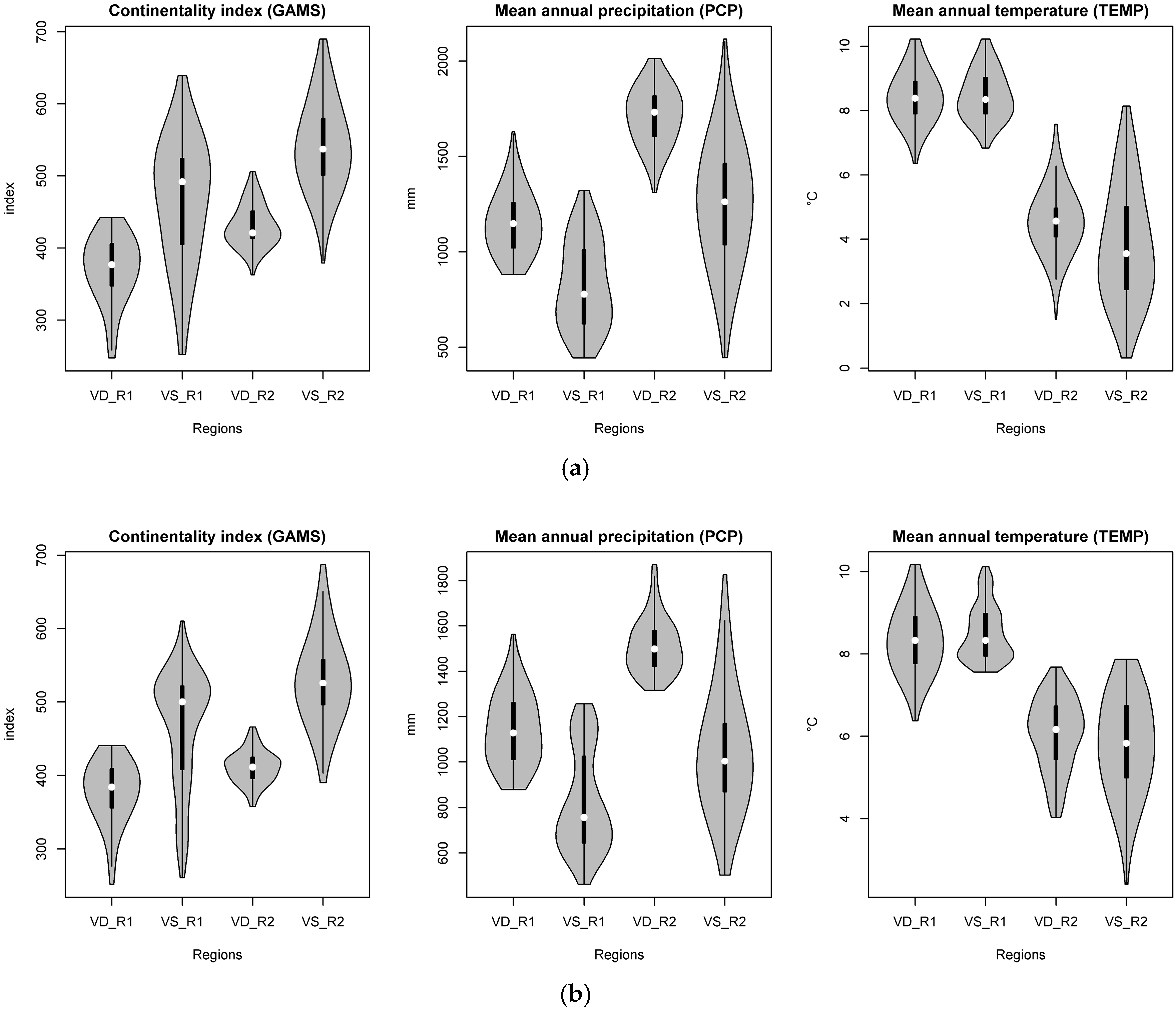
The calibration of each model was executed for a time span of 12 years from 1997 to 2009. First, we determine the number of transitions being modelled in addition to the transitions that describe each scenario (Table 3). For this study we selected to model 15, 11, 15 and 17 transitions for VD_R1, VS_R1, VD_R2, and VS_R2, respectively (Tables S1–S4). The second step is to study how each variable can impact the changes in the landscape we compared to the distribution of the driving forces in each region (Tables S1–S4). Figure 3 shows the results obtained with different driving forces, for the transitions open forest to forest and intensive agriculture to open forest, in the form of violin plots. Significant differences are observed in the frequency distributions of the driving forces for each region, except for the mean annual temperature, which shows similarities between regions at the same altitude range. This finding implies that transitions are influenced by different ranges of the driving forces in each region. The continentality index distribution has similar median values for the regions with the same canton, while the range of values varies between each region belonging to the same canton. While both mean annual precipitation values show considerable variation in each region, the mean annual temperature has similar results for regions in the same elevation band. This finding implies that the separation of the study area into four regions according to an elevation threshold of 900 m a.s.l. and the administrative region (cantons of Vaud and Valais), will allow the development of better land use models.

During the process of calibration, statistically insignificant WoE coefficients from each transition were modified manually [48], based on the low amount of change in certain driving forces ranges of values (Figure S1). The influence of the different driving forces in each region can be observed in the WoE. For example, the results obtained for relationship between the mean annual precipitation and the transition from shrubland to open forest for three regions show that shrubland experiencing a mean annual precipitation of less than 500 mm in VS_R1 is more prone to change than open forest. In regions VD_R2 and VS_R2, shrubland in areas with a mean annual precipitation between 500 mm and 1500 mm is less prone to change to open forest. In addition, for regions VD_R2 and VS_R2 the contrast (difference between the high and low WoE values for the mean annual precipitation) has a strong effect on the transition (Figure S2).

Finally, the correlation between the variables and each land use transition change was tested by means of the Cramer’s coefficient. The results obtained for each region for all land use transitions modelled are less than 0.5, therefore, no variables were discarded [21].

Different settings were tested when calibrating each model and the final parameters used were a 9 × 9 neighbour window and a prune factor of 1.

The most influential drivers change in each region (Tables S1–S4). Bellow 900 m a.s.l., habitation buildings density (POP) and terrain roughness index (TRI) are the most important drivers in VD_R1. Topographic position index (TOPO) and the Euclidean distance to rivers and lakes (DistHydro) were the drivers excluded more often due to the lack of influence over the studied transitions. In VS_R1, the slope angle (SLOPE) is the driver with the highest influence, and the mean annual temperature (TEMP) was the driver excluded more often. Both mean annual solar radiation (MSRAD) and mean annual moisture index (MMIND) showed influence over all of the modelled transitions for both regions. Furthermore, in VS_R1 some transitions have multiple drivers with strong influence. Above 900 m a.s.l., Euclidean distance to rivers and lakes (DistHydro), slope angle (SLOPE), and height above sea level (ELEVATION) are the most influential drivers in VD_R2, while site water balance (SWB) showed the weakest influence over the transitions studied. The slope angle (SLOPE) showed the highest influence over the studied transitions in VS_R2. For both regions above 900 m a.s.l., mean annual temperature (TEMP) showed almost no influence on the transition between intensive and extensive agriculture. The Euclidean distance to rivers and lakes (DistHydro) showed no influence in most of the transitions in VS_R2, while, in VD_R2 it is one of the most influential drivers. Like VS_R1, above 900 m a.s.l., in RS_R2, some transitions have multiple drivers with strong influence. Although mean annual temperature (TEMP) and mean annual precipitation (PCP) are not the most significant drivers over the four regions, they both have some influence. In general, mean annual precipitation (PCP) seems to be a more influential driver. Finally, we observe that glaciers and permanent snow have mean annual solar radiation (MSRAD) and slope angle (SLOPE) has the strongest drivers in VD_R2, with slope angle (SLOPE) and height above sea level (ELEVATION) in VS_R2.

The model performance for each region was assessed based on the fuzzy similarity measurement applied from a pixel-by-pixel to an 11 × 11 neighbourhood window (

Table 4. Fuzzy similarity index for a window size of 1 × 1 and 11 × 11 cells, relative change in area and number of patches.

	VD_R1	VS_R1	VD_R2	VS_R2
Fuzzy Similarity 1 ×1	0.37	0.32	0.45	0.34
Fuzzy Similarity 11 × 11	0.60	0.54	0.77	0.69
Area *	+2%	+7%	+2%	+1%
Number of patches *	−9%	−4.5%	−4%	−4%

* Relative change between the modelled land use for 2009 and the real land use dataset for 2009.

). The minimum similarity fuzzy index obtained for the best models varied from 32% to 45% at a spatial resolution of 1 ha, while at a spatial resolution of 11 ha, the index varies from 54% to 77%. These results indicate that 32% to 45% of the change pixels coincide in both land use maps in a cell-by-cell overlay. At a 1.1 km size window the models reached a similarity between 54% and 77%, meaning that the spatial pattern within a 1.1 km size window have a spatial agreement of 54% in VS_R1 and 77% in VD_R2. According to [23] and similar studies [49,50,51], for the resolution and number of transitions being modelled, the obtained values for the minimum similarity fuzzy index suggest that the models are good and can be used in the simulation of land use change scenarios.

The comparison of the area allocated by the model as well as the number of patches created, shows slight differences between the model and the real dataset (Table 4). These differences are derived from the fact that the yearly amount of change is obtained by the annual transition rates applied iteratively to the land use map [43] and can be observed in the different land use changes.

Table 5. Sample of the transitions modelled for VD_R2. Geometric and quantity comparison between 1997 and the real dataset for 2009, and between the real 1997 and the modelled 2009 dataset. The calibrated model gives similar patches geometries in comparison to the observed one, although we observe some variations concerning the standard deviation.

Transitions
	1→2	1→5	2→1	2→5	4→2	4→5	4→8	5→;1	5→2	5→4	5→6	6→1	6→2	6→5
Mean patch area (ha)	1.46	1.07	1.59	1.10	1.07	2.01	1.11	1.08	1.18	1.63	1.33	1.31	1.12	1.69
	1.47	1.09	1.59	1.08	1.36	2.03	1.36	1.16	1.45	1.38	1.80	1.30	1.21	1.57
Standard deviation patch area	1.23	0.29	2.65	0.38	0.28	2.96	0.34	0.34	0.59	1.24	1.09	0.80	0.39	2.30
	1.28	0.37	2.58	0.30	1.18	3.09	0.95	0.58	1.44	0.98	1.53	0.77	0.61	1.55
Number of patches	1148	297	1516	694	131	352	120	450	996	151	477	467	283	307
	1180	206	1594	751	101	350	102	296	894	164	365	499	298	317
Total area (ha)	1680	317	2411	763	140	708	133	488	1177	246	636	610	316	519
	1740	224	2536	814	137	710	139	343	1299	227	656	651	362	498

1997 to 2009 Obs and 1997 to 2009 Mod. 1—Closed forest; 2—Open forest; 4—Intensive agriculture; 5—Extensive agriculture; 6—Shrubland; 11—Glaciers and permanent snow; 13—Rocks and sand.

depicts a sample of land use transitions modelled for VD_R2, where the small variations can be observed, meaning that the amount of extensive agriculture to change to intensive agriculture in 2009 was obtained from applying the annual transition rates to the 2008 land use map, since the area occupied by extensive agriculture during the time steps evolves due to the interaction with other land uses, as does the area allocated to intensive agriculture.

6.2. Future Scenarios of Land Use Change

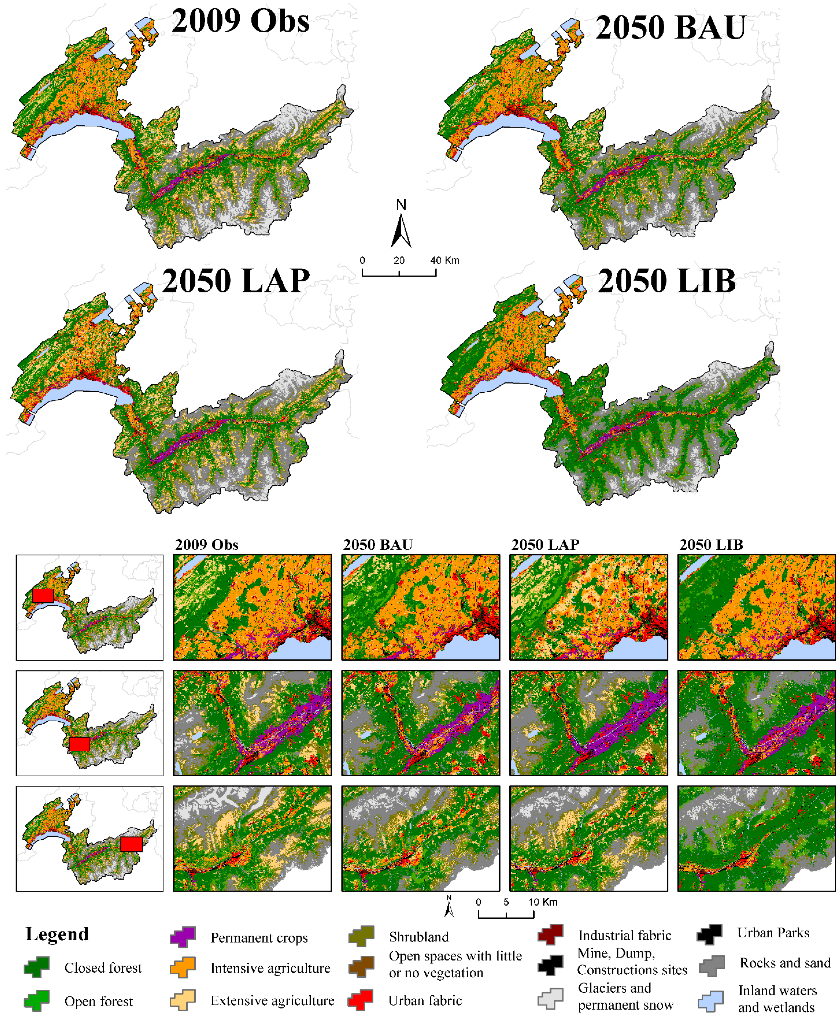
Here we present the results obtained for the three scenarios, each modelled annually for the 41 years from 2009 to 2050 (Figure 4). Projections of future scenarios of land use change are discussed below.

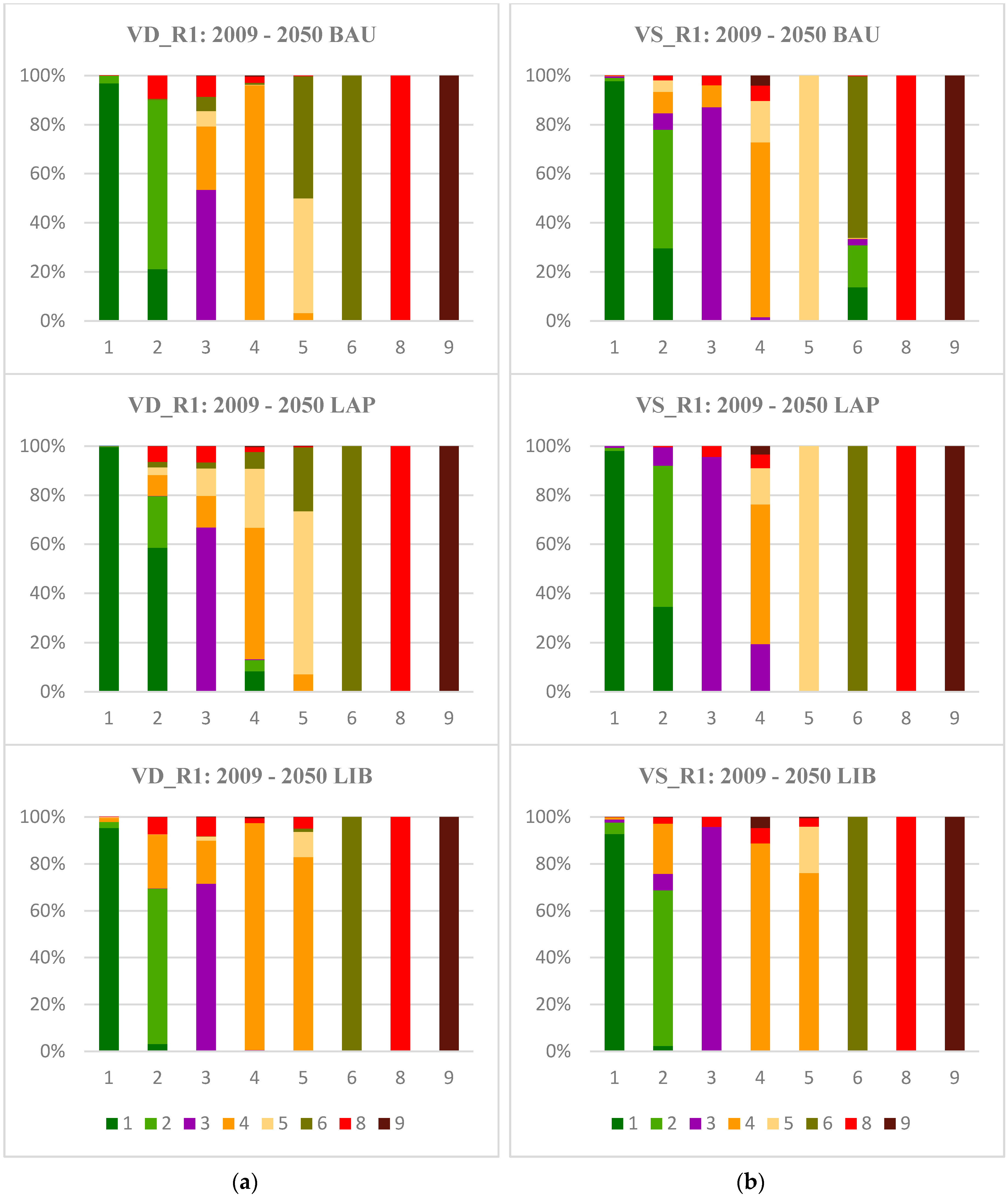
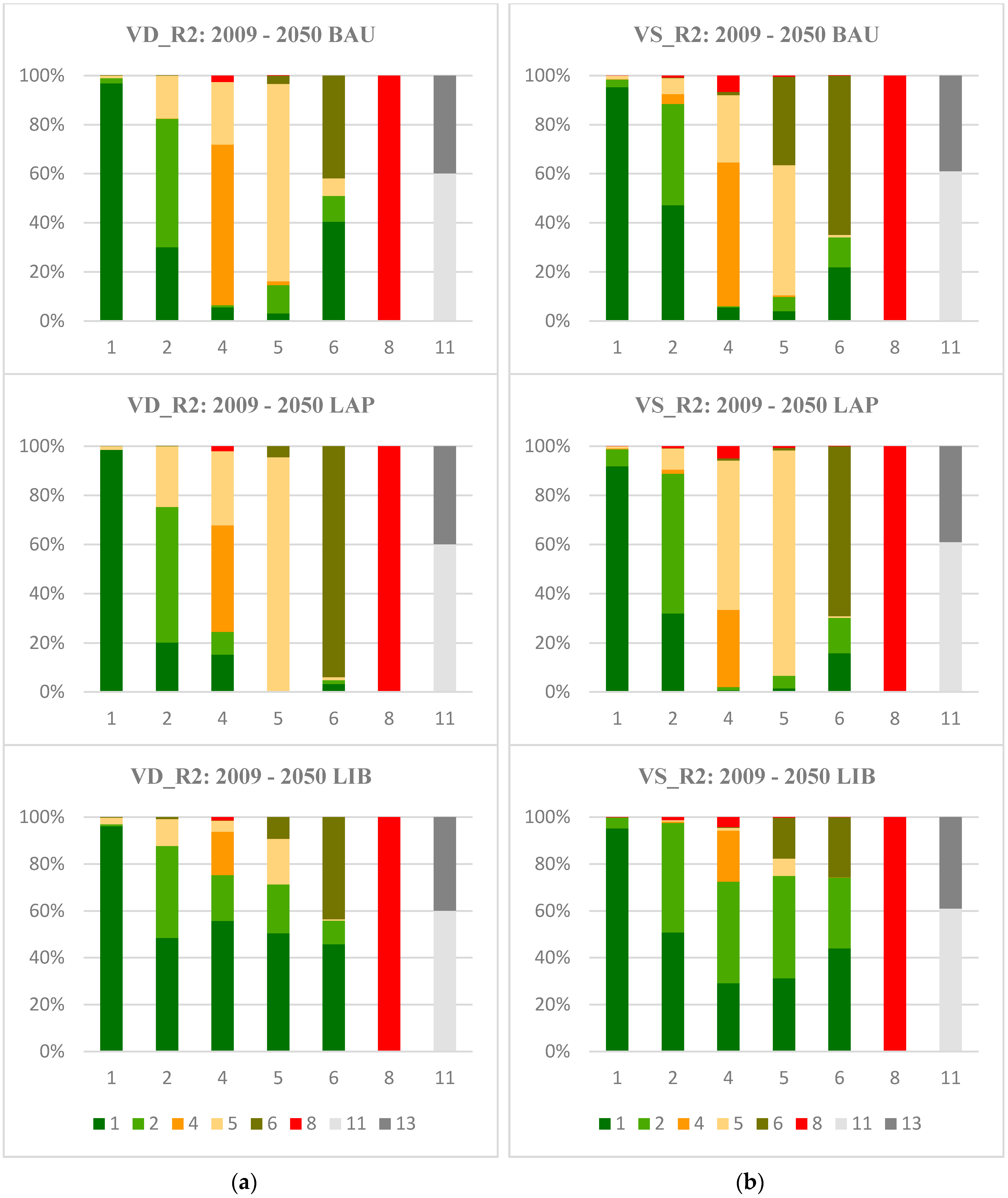
The results of the BAU scenarios in 2050 reflect the long-term effect of the observed changes in the past. Overall, the area occupied by forest, shrubland, and urban have a positive trend (Figure 4 and

Table 6. Total area (ha and %) each LU class occupies in the observed 2009 dataset and in each scenario in 2050. * Classes that were not modelled and, thus, considered static

	2009		BAU		LAP		LIB
LU Class	ha	%	ha	%	ha	%	ha	%
1 closed forest	185,651	22.0	217,391	25.8	211,402	25.1	269,885	32.0
2 open forest	42,651	5.1	41,797	5.0	45,900	5.4	86,788	10.3
3 permanent crops	15,483	1.8	11,597	1.4	12,685	1.5	13,366	1.6
4 intensive agriculture	105,969	12.6	98,725	11.7	58,857	7.0	101,912	12.1
5 extensive agriculture	103,817	12.3	75,468	9.0	130,338	15.5	16,433	2.0
6 shrubland	76,178	9.0	78,597	9.3	65,234	7.7	35,487	4.2
7 open spaces with little or no vegetation *	2113	0.3	2113	0.3	2113	0.3	2113	0.3
8 urban	22,446	2.7	27,993	3.3	27,185	3.2	27,595	3.3
9 industry	3125	0.4	3,752	0.4	3719	0.4	3854	0.5
10 mine, dump, construction sites and Transport units *	19,613	2.3	19,613	2.3	19,613	2.3	19,613	2.3
11 glaciers and permanent snow	67,591	8.0	41,226	4.9	41,226	4.9	41,226	4.9
12 urban Parks *	3218	0.4	3218	0.4	3218	0.4	3218	0.4
13 rocks and sand *	145,024	17.2	171,389	20.3	171,389	20.3	171,389	20.3
14 inland waters and wetlands *	49,345	5.9	49,345	5.9	49,345	5.9	49,345	5.9

). In VD_R1 shows a high increase of shrubland (

Table 7. Total area (ha and %) each LU class occupies in the observed 2009 dataset and in each scenario in 2050. The percentage of total area (%) was calculated with the area occupied by each region: 210,150 ha, 45,874 ha, 110,705 ha and 475,495 ha, respectively.

	Land Use	2009 Obs		2050 BAU		2050 LAP		2050 LIB
		ha	%	ha	%	ha	%	ha	%
VD_R1	closed forest	38,442	18.3	38,556	18.3	48,244	23.0	36,780	17.5
	open forest	5300	2.5	4959	2.4	5014	2.4	4528	2.2
	permanent crops	6797	3.2	3639	1.7	4749	2.3	5351	2.5
	intensive agriculture	81,731	38.9	80,259	38.2	45,909	21.8	91,491	43.5
	extensive agriculture	11,178	5.3	5883	2.8	27,994	13.3	1482	0.7
	shrubland	265	0.1	6855	3.3	8991	4.3	437	0.2
	urban	12,746	6.1	15,980	7.6	15,264	7.3	15,980	7.6
	industry	1775	0.8	2103	1.0	2069	1.0	2185	1.0
VS_R1	closed forest	12,565	27.4	13,081	28.5	12,955	28.2	12,955	28.2
	open forest	2184	4.8	1423	3.1	1222	2.7	1222	2.7
	permanent crops	8445	18.4	7717	16.8	7695	16.8	774	16.9
	intensive agriculture	7139	15.6	6062	13.2	6058	13.2	7728	14.6
	extensive agriculture	1054	2.3	2366	5.2	2334	5.1	6684	3.4
	shrubland	1125	2.5	741	1.6	1125	2.5	1582	2.5
	urban	3859	8.4	4682	10.2	4682	10.2	4710	10.3
	industry	1182	2.6	1481	3.2	1482	3.2	1501	3.3
VD_R2	closed forest	49,629	44.8	54,333	49.1	52,026	47.0	73,007	65.9
	open forest	9711	8.8	10,125	9.1	6031	5.4	12,069	10.9
	intensive agriculture	6448	5.8	4667	4.2	2787	2.5	1192	1.1
	extensive agriculture	28,946	26.1	27,472	24.8	32,737	29.6	8485	7.7
	shrubland	5220	4.7	3185	2.9	6239	5.6	5109	4.6
	urban	1645	1.5	1817	1.6	1779	1.6	1737	1.6
	glaciers and permanent snow	326	0.3	196	0.2	196	0.2	196	0.2
	rocks and sand	5136	4.6	5266	4.8	5266	4.8	5266	4.8
VS_R2	closed forest	85,015	17.9	111,421	23.4	98,177	20.6	147,143	30.9
	open forest	25,456	5.4	25,290	5.3	33,633	7.1	68,969	14.5
	intensive agriculture	10,651	2.2	7737	1.6	4103	0.9	2545	0.5
	extensive agriculture	62,639	13.2	39,747	8.4	67,273	14.1	4884	1.0
	shrubland	69,568	14.6	67,816	14.3	48,879	10.3	28,816	6.1
	urban	4196	0.9	5514	1.2	5460	1.1	5168	1.1
	glaciers and permanent snow	67,265	14.1	41,030	8.6	41,030	8.6	41,030	8.6
	rocks and sand	139,109	29.3	165,344	34.8	165,344	34.8	165,344	34.8

) mainly caused by the abandonment and fragmentation of extensive agriculture, with an increase in the number of patches and decreasing mean patch size (Figure 5 and

Table 8. Landscape fragmentation parameters for VD_R1: number of patches (NP), mean patch area (MPA) in ha, and standard deviation of the mean patch area, in 2009 and 2050 for each scenario and land use type.

	VD_R1	1	2	3	4	5	6	8	9
Number of patches (NP)	2009	1777	3498	1721	1295	3587	199	2548	595
	BAU	1773	2660	662	1090	2290	1693	2275	702
	LAP	1823	2229	907	1176	2385	885	2311	689
	LIB	1847	2380	997	962	670	265	2253	722
Mean patch area (MPA) ha	2009	21.6	1.5	3.9	63.1	3.1	1.3	5.0	3.0
	BAU	21.7	1.9	5.5	73.6	2.5	4.0	7.0	3.0
	LAP	26.4	2.2	5.2	39.0	11.7	10.1	6.6	3.0
	LIB	19.9	1.9	5.4	95.1	2.2	1.6	7.1	3..0
Standard deviation patch area	2009	129	1.3	31	1460.8	4.5	1.6	37	5.3
	BAU	134.8	5.3	33.1	1628.8	3.8	8.0	57.6	6.5
	LAP	233.8	3.4	38.3	374.2	91.5	32.1	55.0	6.5
	LIB	123.1	4.0	37.8	2301.8	3.1	2.7	57.9	6.9

1: closed forest; 2: open forest; 3: permanent crops; 4: intensive agriculture; 5: extensive agriculture; 6: shrubland; 8: urban; 9: industrial.

). In VS_R1, the increase of closed forest and extensive agriculture was accompanied by the decrease of open forest, permanent crops, intensive agriculture and shrubland (Table 7 and Figure 5). We also observe a reduction of the number of patches for all landscapes with an increase of the mean patch size for the majority of the land use, resulting in a less fragmented landscape (

Table 9. Landscape fragmentation parameters for VS_R1: number of patches (NP), mean patch area (MPA) in ha, and standard deviation of the mean patch area, in 2009 and 2050 for each scenario and land use type.

	VS_R1	1	2	3	4	5	6	8	9
Number of patches (NP)	2009	616	1378	582	1057	598	577	805	340
	BAU	544	798	588	627	784	350	690	360
	LAP	548	707	608	642	785	577	691	360
	LIB	557	728	609	757	698	577	688	363
Mean patch area (MPA) ha	2009	20.4	1.6	14.5	6.8	1.8	1.9	4.8	3.5
	BAU	24.0	1.8	13.1	9.7	3.0	2.1	6.8	4.1
	LAP	23.6	1.7	12.6	9.4	2.9	1.9	6.8	4.1
	LIB	23.3	1.7	12.8	8.8	2.3	1.9	6.8	4.1
Standard deviation patch area	2009	130.4	1.3	110.7	48.7	1.6	3.2	12.6	8.4
	BAU	177.8	2.2	110.1	65.7	8.0	3.5	25.5	11.3
	LAP	161.2	2.0	96.4	64.5	7.7	3.2	25.5	11.3
	LIB	159.1	1.9	96.7	59.6	4.8	3.2	25.5	11.5

1: closed forest; 2: open forest; 3: permanent crops; 4: intensive agriculture; 5: extensive agriculture; 6: shrubland; 8: urban; 9: industrial.

). Both VD_R2 and VS_R2 regions show similar changes, with the increase in area of closed forest and open forest, due to the loss of agriculture (intensive and extensive) and shrubland (Figure 6 and Figure 7, Table 7).

The LAP scenario is the most similar to the BAU scenario. Nonetheless, with higher rates of change for the loss of intensive agriculture and opposite trends for the extensive agriculture. Overall the LAP scenario results in the increase of forest (closed and open forest) and extensive agriculture, due to the loss of permanent crops and intensive agriculture (Table 7, Figure 5 and Figure 6). In comparison to the BAU scenario, the LAP scenario results in proportionally greater changes in the landscape, with ~5% decrease of intensive and ~7% increase of extensive agriculture area (Table 6). A closer look at the regional level reveals a different trend from the one observed in the BAU scenario, with the most noticeable change in the landscape occurring in VD_R1, with the reduction in the area occupied by intensive agriculture from 38.9% to 21.8% (Table 7). Under the LAP scenario, we observe an increase of closed forest and a high increase of both extensive agriculture and shrubland in VD_R1 (Table 7). VS_R1 shows similar results for the amount of change and landscape fragmentation as in the BAU scenario. The LAP scenario applied to VD_R2 and VS_R2 results in the loss of intensive agriculture (Table 7), mostly to extensive agriculture (Figure 6). An increase of ~5% and ~6% of the area occupied by extensive agriculture was observed. Additionally, a decrease in the number of patches is observed, as well as the increase in the mean patch area and standard deviation, with the highest increase observed in VD_R2 (

Table 10. Landscape fragmentation parameters for VD_R2: number of patches (NP), mean patch area (MPA) in ha, and standard deviation of the mean patch area, in 2009 and 2050 for each scenario and land use type.

	VD_R2	1	2	4	5	6	8	11	13
Number of patches (NP)	2009	996	3753	472	1459	1248	588	26	525
	BAU	878	1647	359	1306	322	560	18	522
	LAP	888	2066	317	1234	958	567	19	522
	LIB	416	1493	250	466	595	570	20	522
Mean patch area (MPA) ha	2009	49.8	2.6	13.7	19.8	4.2	2.8	12.5	9.8
	BAU	61.9	6.1	13.0	21.0	9.9	3.2	10.9	10.1
	LAP	58.6	2.9	8.8	26.5	6.5	3.1	10.3	10.1
	LIB	175.5	8.1	4.8	18.2	8.6	3.0	9.8	10.1
Standard deviation patch area	2009	729.0	9.9	39.8	97.2	12.2	8.3	22.6	92.1
	BAU	961.4	83.2	49.6	128.7	42.9	12.1	19.1	96.8
	LAP	867.9	11.8	28.9	158.6	34.6	11.5	18.7	96.8
	LIB	2254.3	56.2	18.0	72.8	42.4	10.9	17.1	96.8

1: closed forest; 2: open forest; 4: intensive agriculture; 5: extensive agriculture; 6: shrubland; 8: urban; 11: glaciers and permanent snow; 13: rocks and sand.

).

The LIB scenario is characterised by the abandonment of agriculture (both intensive and extensive) with an increase of the forest cover above 900 m a.s.l., and below 900 m a.s.l. the scenario is characterised by the conversion from extensive to intensive agriculture. The results obtained for the complete study area show that both closed and open forest grow significantly, from 22.0% in 2009 to 32.0% and from 5.1% to 10.3%, respectively (Table 6). While the presence of extensive agriculture decreases from 12.3% in 2009 to 2.0% in 2050 (Table 6). At regional levels below 900 m a.s.l., in contrast to the BAU scenario, the abandonment of extensive agriculture is mostly due to the conversion to intensive agriculture (Figure 4 and Figure 5). In VD_R1, we observed a decrease of the number of patches for intensive agriculture, along with the increase of both the mean patch size and standard deviation; mostly due to the transition of 80% from extensive agriculture into intensive agriculture (Table 8 and Figure 5). Above 900 m a.s.l. the LIB scenario results in the high increase of forest area (Figure 6 and Figure 7, Table 7). Almost all agriculture above 900 m a.s.l. will be converted into closed and open forest by 2050 (Figure 6). Closed and open forest increases significantly in VD_R2 and VS_R2, in comparison to the area observed in 2009 (Table 7). In addition to the growth in the area of both closed and open forest, the number of patches decreases and the mean patch size increase, resulting in the conversion of large patches of closed and open forest (Table 10 and

Table 11. Landscape fragmentation parameters for VS_R2: number of patches (NP), mean patch area (MPA) in ha, and standard deviation of the mean patch area, in 2009 and 2050 for each scenario and land use type.

	VS_R2	1	2	4	5	6	8	11	13
Number of patches (NP)	2009	2351	8421	1488	4918	8861	1471	1120	5710
	BAU	1723	6544	1141	4707	4319	1373	870	5504
	LAP	2069	6841	786	4425	6932	1380	872	5506
	LIB	2287	6000	630	1690	3393	1368	856	5499
Mean patch area (MPA) ha	2009	36.2	3.0	7.2	12.7	7.9	2.9	60.1	24.4
	BAU	64.7	3.9	6.7	8.4	15.7	4.0	47.2	30.0
	LAP	47.5	4.9	5.2	15.2	7.1	4.0	47.1	30.0
	LIB	64.3	11.5	4.0	2.9	8.5	3.8	47.9	30.1
Standard deviation patch area	2009	406.8	6.7	33.9	65.4	44.6	7.7	672.9	540.1
	BAU	848.1	11.9	34.0	41.1	121.3	14.2	411.6	1181.1
	LAP	541.5	19.0	25.9	68.6	30.8	12.6	415.1	1181.5
	LIB	1019.5	60.3	22.2	5.8	43.4	11.3	415.9	1182.3

1: closed forest; 2: open forest; 4: intensive agriculture; 5: extensive agriculture; 6: shrubland; 8: urban; 11: glaciers and permanent snow; 13: rocks and sand.

). The increase of forest is accompanied by the loss of intensive and extensive agriculture (Figure 6).

Urban was modelled with the same amount of change in all scenarios, for each region. In VD_R1, the increase of urban area results mostly from the loss of open forest and permanent crops. In VS_R1, permanent crops and intensive agriculture area are transformed into urban area. Above 900 m a.s.l. urban area increases at the cost of intensive agriculture. Although the three scenarios are models with the same amount of change, we observe some variation on the area allocated across scenarios for the same regions (Table 7). These differences are derived from the fact that the yearly amount of change is obtained by the annual transition rates applied iteratively to the land use map [43], meaning that the amount of intensive agriculture to change to urban area in 2050 was obtained from applying the annual transition rates to the 2049 land use map, since the area occupied by intensive agriculture during the time steps evolves at different rates between scenarios, so does the area allocated to urbanization.

The total area lost by the Glaciers and permanent snow represents ~40% of the area obtain in 2009 (Table 6 and Figure 7), equivalent to 130 ha in VD_R2 and 26,235 ha in VS_R2. Glaciers and permanent snow modelled in this study show an increase of fragmentation mostly in VS_R2 (Table 10 and Table 11), with small variations between scenarios in the patch geometry. These small variations are derived from how the patch geometry is defined in both Expander and Patcher allocation rules. In contrast to the urban land use, the area allocated in each scenario for the glaciers and permanent snow is the same (Table 7) between scenarios. The differences between these two land uses is the fact that glaciers and permanent snow does not gain area from other land uses, meaning that they evolve at the same rate year after year.

7. Discussion and Conclusions

This study generates scenarios of land use change in a mountainous region of Switzerland using Dinamica EGO software. Our results showed that key important drivers for explaining the transition between a given set of land use classes varies across the regions (Tables S1–S4), however the relative importance of slope within each region was observed. Our results show that both mean temperature and precipitation are not the most significant drivers over the four regions, however, they both have some influence. These results indicate the importance of creating regional models in agreement with a previous study [26].

The results obtained for the different regions in each scenario show significant differences, with the LIB scenario being the one with the highest impact. The BAU scenario results in a considerable change in the landscape across regions, however compared to LAP, which is otherwise similar, these changes have less impact on the landscape. The LAP scenario suggests an increase of the overall proportion of extensive agriculture from 9.0%, in the BAU scenario to 15.5%, in the LAP scenario (Table 6). Such changes will increase the potential for habitat areas [13,14,15], however, it could accelerate soil erosion, mostly at high altitudes according to previous studies [6,7]. The marked increase in forest cover from the LIB scenario in association with the glaciers and permanent snow loss of ~40%, is expected to decrease the amount of runoff resulting in a clear impact on the quantity and quality of water [11,12,13,52,53]. According to [16] the increase of forest area along with the increase of temperature, will most probably raise the occurrences of fires in the regions located in Valais. Although the loss of extensive agriculture is also expected to be a threat to animal and plant species [13,14,15] , different studies suggest that extensive agriculture abandonment could allow the implementation of landscape planning strategies at lower costs [54,55]. Although care must be taken when using scenarios due to limitations on the explanatory power of the driving forces [28,31,34], as well as changes in government legislation and land management that impact land use change. However, scenarios of land use/land cover change offer the possibility to evaluate potential impacts and improve planning [2,5].

The land use change model applied in this study incorporates a statistical inference method (WoE) and we model multiple land use transitions as compared with previous studies [13,25,26,27]. Nevertheless, several improvements can be implemented. The aggregation of land use categories is still a limitation for modelling due to the amount of information that each driving force can provide to the model. The main challenge remains that of handling the SFSO land use datasets. Each dataset was obtained from aerial surveys, which took approximately 12 years to be completed, although the sequence between datasets was the same for the most part of the territory. A possible improvement would be the replacing of the land use dataset by land use data obtained from satellite imagery [4,17,22,27,56]. Burgi [28] reported that the different rates of land use change and temporal trajectories should be taken into account and divided into: “constantly slow” and “constantly rapid change”; “accelerating change” and “decelerating change”; “isolated rapid change in the distant past”; and “isolated near rapid change in the near past”. Although this type of information is supported by Dinamica EGO, it is extremely difficult to gather and is not consistent with the type of land use dataset available for this study. Finally, the model does not consider climatic variations of precipitation; only the expected 2 °C increase of the mean observed temperature by 2050 [47] was implemented. The expected variations in precipitation and temperature can affect reforestation patterns and dynamics, as well as the glaciers [57], and should be implemented in future studies.

References

1. Lambin, E.F.; Meyfroidt, P. Global land use change, economic globalization, and the looming land scarcity. Proc. Natl. Acad. Sci. USA 2011, 108, 3465–3472. [Google Scholar] [CrossRef] [PubMed]
2. Mancosu, E.; Gago-Silva, A.; Barbosa, A.; de Bono, A.; Ivanov, E.; Lehmann, A.; Fons, J. Future land-use change scenarios for the Black Sea catchment. Environ. Sci. Policy 2014, 46, 26–36. [Google Scholar] [CrossRef]
3. Verburg, P.H.; Schulp, C.J.E.; Witte, N.; Veldkamp, A. Downscaling of land use change scenarios to assess the dynamics of European landscapes. Agric. Ecosyst. Environ. 2006, 114, 39–56. [Google Scholar] [CrossRef]
4. Veldkamp, A.; Lambin, E.F. Predicting land-use change. Agric. Ecosyst. Environ. 2001, 85, 1–6. [Google Scholar] [CrossRef]
5. Verburg, P.H.; Overmars, K.P. Combining top-down and bottom-up dynamics in land use modeling: Exploring the future of abandoned farmlands in Europe with the dyna-clue model. Landsc. Ecol. 2009, 24, 1167–1181. [Google Scholar] [CrossRef]
6. Maeda, E.E.; Pellikka, P.K.E.; Siljander, M.; Clark, B.J.F. Potential impacts of agricultural expansion and climate change on soil erosion in the Eastern ARC Mountains of Kenya. Geomorphology 2010, 123, 279–289. [Google Scholar] [CrossRef]
7. Wolf, S.; Walz, U.; Kleber, A. Effects of land-cover change on soil erosion in the saxon Switzerland National Park region. Erde 2009, 140, 155–174. [Google Scholar]
8. Soares-Filho, B.S.; Cerqueira, G.C.; Pennachin, C.L. Dinamica—A stochastic cellular automata model designed to simulate the landscape dynamics in an Amazonian Colonization Frontier. Ecol. Model. 2002, 154, 217–235. [Google Scholar] [CrossRef]
9. Temme, A.J.A.M.; Claessens, L.; Veldkamp, A.; Schoorl, J.M. Evaluating choices in multi-process landscape evolution models. Geomorphology 2011, 125, 271–281. [Google Scholar] [CrossRef]
10. Kundzewicz, Z.W.; Mata, L.J.; Arnell, N.W.; Döll, P.; Kabat, P.; Jiménez, B.; Miller, K.A.; Oki, T.; Sen, Z.; Shiklomanov, I.A. Freshwater Resources and Their Management. Climate Change 2007: Impacts, Adaptation and Vulnerability; Cambridge University Press: Cambridge, UK, 2007. [Google Scholar]
11. Morán-Tejeda, E.; Ceballos-Barbancho, A.; Llorente-Pinto, J.; López-Moreno, J. Land-cover changes and recent hydrological evolution in the Duero Basin (Spain). Reg. Environ. Chang. 2012, 12, 17–33. [Google Scholar] [CrossRef]
12. Rahman, K.; da Silva, A.G.; Tejeda, E.M.; Gobiet, A.; Beniston, M.; Lehmann, A. An independent and combined effect analysis of land use and climate change in the upper Rhone River Watershed, Switzerland. Appl. Geogr. 2015, 63, 264–272. [Google Scholar] [CrossRef]
13. Bolliger, J.; Kienast, F.; Soliva, R.; Rutherford, G. Spatial sensitivity of species habitat patterns to scenarios of land use change (Switzerland). Landsc. Ecol. 2007, 22, 773–789. [Google Scholar] [CrossRef]
14. Laiolo, P.; Dondero, F.; Ciliento, E.; Rolando, A. Consequences of pastoral abandonment for the structure and diversity of the Alpine avifauna. J. Appl. Ecol. 2004, 41, 294–304. [Google Scholar] [CrossRef]
15. Kampmann, D.; Herzog, F.; Jeanneret, P.; Konold, W.; Peter, M.; Walter, T.; Wildi, O.; Lüscher, A. Mountain grassland biodiversity: Impact of site conditions versus management type. J. Nat. Conserv. 2008, 16, 12–25. [Google Scholar] [CrossRef]
16. Zumbrunnen, T.; Bugmann, H.; Conedera, M.; Buergi, M. Linking forest fire regimes and climate—A historical analysis in a dry inner Alpine Valley. Ecosystems 2009, 12, 73–86. [Google Scholar] [CrossRef]
17. Schneeberger, N.; Buergi, M.; Hersperger, A.M.; Ewald, K.C. Driving forces and rates of landscape change as a promising combination for landscape change research—An application on the northern fringe of the Swiss Alps. Land Use Policy 2007, 24, 349–361. [Google Scholar] [CrossRef]
18. Houet, T.; Verburg, P.H.; Loveland, T.R. Monitoring and modelling landscape dynamics. Landsc. Ecol. 2010, 25, 163–167. [Google Scholar] [CrossRef]
19. Bürgi, M.; Hersperger, A.; Schneeberger, N. Driving forces of landscape change—Current and new directions. Landsc. Ecol. 2004, 19, 857–868. [Google Scholar] [CrossRef]
20. Verburg, P.H.; van Eck, J.R.R.; de Nijs, T.C.M.; Dijst, M.J.; Schot, P. Determinants of land-use change patterns in The Netherlands. Environ. Plan. B Plan. Des. 2004, 31, 125–150. [Google Scholar] [CrossRef]
21. De Almeida, C.M.; Batty, M.; Monteiro, A.M.V.; Camara, G.; Soares-Filho, B.S.; Cerqueira, G.C.; Pennachin, C.L. Stochastic cellular automata modeling of urban land use dynamics: Empirical development and estimation. Comput. Environ. Urban Syst. 2003, 27, 481–509. [Google Scholar] [CrossRef]
22. Irwin, E.G.; Geoghegan, J. Theory, data, methods: Developing spatially explicit economic models of land use change. Agric. Ecosyst. Environ. 2001, 85, 7–24. [Google Scholar] [CrossRef]
23. Soares-Filho, B.S.; Rodrigues, H.; Costa, W. Modeling Environmental Dynamics with Dinamica Ego. Available online: http://www.csr.ufmg.br/dinamica/tutorial/Dinamica_EGO_guidebook.pdf (accessed on 28 April 2016).
24. Verbunt, A.; Zwaaftink, M.G.; Gurtz, J. The hydrologic impact of land cover changes and hydropower stations in the Alpine Rhine Basin. Ecol. Model. 2005, 187, 71–84. [Google Scholar] [CrossRef]
25. Walz, A. Land Use Modelling for an Integrated Approach to Regional Development in the Swiss Alps. Ph.D. Thesis, University of Zurich, Zurich, Switzerland, 2006. [Google Scholar]
26. Price, B.; Kienast, F.; Seidl, I.; Ginzler, C.; Verburg, P.H.; Bolliger, J. Future landscapes of Switzerland: Risk areas for urbanisation and land abandonment. Appl. Geogr. 2015, 57, 32–41. [Google Scholar] [CrossRef]
27. Rutherford, G.N.; Bebi, P.; Edwards, P.J.; Zimmermann, N.E. Assessing land-use statistics to model land cover change in a mountainous landscape in the European Alps. Ecol. Model. 2008, 212, 460–471. [Google Scholar] [CrossRef]
28. Burgi, M. A case study of forest change in the Swiss Lowlands. Landsc. Ecol. 1999, 14, 567–575. [Google Scholar] [CrossRef]
29. Regmi, N.R.; Giardino, J.R.; Vitek, J.D. Modeling susceptibility to landslides using the weight of evidence approach: Western Colorado, USA. Geomorphology 2010, 115, 172–187. [Google Scholar] [CrossRef]
30. Roberts, M.C.; Randolph, J.C.; Chiesa, J.R. Land suitability model for the evaluation of land-use change. Environ. Manag. 1979, 3, 339–352. [Google Scholar] [CrossRef]
31. Gellrich, M.; Baur, P.; Koch, B.; Zimmermann, N.E. Agricultural land abandonment and natural forest re-growth in the Swiss mountains: A spatially explicit economic analysis. Agric. Ecosyst. Environ. 2007, 118, 93–108. [Google Scholar] [CrossRef]
32. Jopp, F.; Reuter, H.; Breckling, B.; Müller, F. What are the general conditions under which ecological models can be applied? In Modelling Complex Ecological Dynamics; Springer: Berlin/Heidelberg, Germany, 2011; pp. 13–28. [Google Scholar]
33. VanDerWal, J.; Falconi, L.; Januchowski, S.; Shoo, L.; Storlie, C. Sdmtools: Species Distribution Modelling Tools: Tools for Processing Data Associated with Species Distribution Modelling Exercises. R Package Version 1.1-221. Available online: http://cran.r-project.org/package=SDMTools (accessed on 28 April 2016).
34. Rutherford, G.N.; Guisan, A.; Zimmermann, N.E. Evaluating sampling strategies and logistic regression methods for modelling complex land cover changes. J. Appl. Ecol. 2007, 44, 414–424. [Google Scholar] [CrossRef]
35. Soares-Filho, B.S.; Rodrigues, H.; Costa, W.; Ferreira, B.; Machado, R.; Figueira, D. Dinamica Ego; Universidade Federal de Minas Gerais: Belo Horizonte-MG, Brazil, 2013. [Google Scholar]
36. Meteoswiss. Available online: www.meteoswiss.ch (accessed on 1 September 2015).
37. Nippel, T.; Klingl, T. Swiss Land Use in the European Context. Integration of Swiss Land Use Statistics with Corine Land Cover; Swiss Federal Statistical Office (SFSO): Neuchâtel, Switzerland, 1998. [Google Scholar]
38. Weed, D.L. Weight of evidence: A review of concept and methods. Risk Anal. 2005, 25, 1545–1557. [Google Scholar] [CrossRef] [PubMed]
39. Wilson, M.F.J.; O’Connell, B.; Brown, C.; Guinan, J.C.; Grehan, A.J. Multiscale terrain analysis of multibeam bathymetry data for habitat mapping on the continental slope. Mar. Geodesy 2007, 30, 3–35. [Google Scholar] [CrossRef]
40. Federal office for agriculture. Available online: http://www.blw.admin.ch/index.html?lang=en (accessed on 1 September 2015).
41. Mas, J.-F.; Kolb, M.; Houet, T.; Paegelow, M.; Olmedo, M.C. Una comparación de diferentes enfoques de modelación de cambios de cobertura/uso del suelo. In Proceedings of the XIV Simposio Internacional SELPER 2010, Guanajuato, Mexico, 8 November 2010. [Google Scholar]
42. Kolb, M.; Mas, J.-F.; Galicia, L. Evaluating drivers of land-use change and transition potential models in a complex landscape in Southern Mexico. Int. J. Geogr. Inf. Sci. 2013, 27, 1804–1827. [Google Scholar] [CrossRef]
43. Mas, J.-F.; Kolb, M.; Paegelow, M.; Camacho Olmedo, M.T.; Houet, T. Inductive pattern-based land use/cover change models: A comparison of four software packages. Environ. Model. Softw. 2014, 51, 94–111. [Google Scholar] [CrossRef]
44. Jopp, F.; Reuter, H.; Breckling, B.; Lange, C.; Weigmann, G. How valid are model results? Assumptions, validity range and documentation. In Modelling Complex Ecological Dynamics; Springer: Berlin/Heidelberg, Germany, 2011; pp. 323–340. [Google Scholar]
45. Hagen-Zanke, A. Fuzzy set approach to assessing similarity of categorical maps. Int. J. Geogr. Inf. Sci. 2003, 17, 235–249. [Google Scholar] [CrossRef]
46. Costanza, R. Model goodness of fit—A multiple resolution procedure. Ecol. Model. 1989, 47, 199–215. [Google Scholar] [CrossRef]
47. Organe consultatif sur les Changements Climatiques (OcCC). Expected Impacts on Environment, Society And Economy; OcCC: Berne, Switzerland, 2007. [Google Scholar]
48. Pérez-Vega, A.; Mas, J.-F.; Ligmann-Zielinska, A. Comparing two approaches to land use/cover change modeling and their implications for the assessment of biodiversity loss in a deciduous tropical forest. Environ. Model. Softw. 2012, 29, 11–23. [Google Scholar] [CrossRef]
49. Maeda, E.E.; de Almeida, C.M.; de Carvalho Ximenes, A.; Formaggio, A.R.; Shimabukuro, Y.E.; Pellikka, P. Dynamic modeling of forest conversion: Simulation of past and future scenarios of rural activities expansion in the fringes of the Xingu National Park, Brazilian Amazon. Int. J. Appl. Earth Obs. Geoinf. 2011, 13, 435–446. [Google Scholar] [CrossRef]
50. Yanai, A.M.; Fearnside, P.M.; Graça, P.M.L.D.A.; Nogueira, E.M. Avoided deforestation in Brazilian Amazonia: Simulating the effect of the Juma Sustainable Development Reserve. For. Ecol. Manag. 2012, 282, 78–91. [Google Scholar] [CrossRef]
51. Salonen, M.; Maeda, E.E.; Toivonen, T. Evaluating the impact of distance measures on deforestation simulations in the fluvial landscapes of Amazonia. Ambio 2014, 43, 779–790. [Google Scholar] [CrossRef] [PubMed]
52. Beniston, M. Climatic change in mountain regions: A review of possible impacts. Clim. Chang. 2003, 59, 5–31. [Google Scholar] [CrossRef]
53. Kundzewicz, Z.W.; Mata, L.J.; Arnell, N.W.; Döll, P.; Kabat, P.; Jiménez, B.; Miller, K.A.; Oki, T.; Sen, Z.; Shiklomanov, I.A. Freshwater resources and their management. Contribution of working group ii to the fourth assessment report of the intergovernmental panel on climate change. In Climate Change 2007: Impacts, Adaptation and Vulnerability; Parry, O.F.C., Palutikof, P.J., van der Hanson, L.A.C.E., Eds.; Cambridge University Press: Cambridge, UK, 2007. [Google Scholar]
54. Grau, R.; Kuemmerle, T.; Macchi, L. Beyond ‘land sparing versus land sharing’: Environmental heterogeneity, globalization and the balance between agricultural production and nature conservation. Curr. Opin. Environ. Sustain. 2013, 5, 477–483. [Google Scholar] [CrossRef]
55. Navarro, L.M.; Pereira, H.M. Towards a european policy for rewilding. In Rewilding European Landscapes; Pereira, H.M., Navarro, L.M., Eds.; Springer International Publishing: Cham, Switzerland, 2015; pp. 205–223. [Google Scholar]
56. Koomen, E.; Stillwell, J.; Bakema, A.; Scholten, H.; Verburg, P.H.; Overmars, K.P. Dynamic simulation of land-use change trajectories with the clue-s model. In Modelling Land-Use Change; Springer: Dordrecht, The Netherlands, 2007; Volume 90, pp. 321–337. [Google Scholar]
57. López-Moreno, J.I.; Goyette, S.; Vicente-Serrano, S.M.; Beniston, M. Effects of climate change on the intensity and frequency of heavy snowfall events in the pyrenees. Clim. Chang. 2011, 105, 489–508. [Google Scholar] [CrossRef]
Figure 1. Study area and modelled regions: canton of Vaud bellow 900 m a.s.l. (VD_R1), canton of Vaud above 900 m a.s.l. (VD_R2), canton of Valais bellow 900 m a.s.l. (VS_R1) and canton of Valais above 900 m a.s.l. (VS_R2).
Ijgi 06 00115 g001
Figure 2. Flow chart illustrating the land use/cover change Dinamica Environment for Geoprocessing Objects (EGO) modelling framework.
Ijgi 06 00115 g002
Figure 3. Violin plots for the driving forces distribution in each region. The median is shown as a white circle, the wide black bars represent the interquartile range, the range of values is represented by the thin vertical line, and the shaded areas represent the frequency distribution in each region. (a) transition from open forest (1997) to closed forest (2009); (b) transition from intensive agriculture (1997) to open forest (2009).
Ijgi 06 00115 g003
Figure 4. Observed land use in 2009 and results from Dinamica EGO model simulation showing the landscape composition for the year 2050 in each scenario (business-as-usual (BAU), LAP, and LIB).
Ijgi 06 00115 g004
Figure 5. Percentage of land use composition in 2050 (BAU, LAP and LIB scenarios) out of the existent in 2009, in (a) VD_R1 and (b) VS_R1. Each stacked bar represents the share of land use type in 2050 (BAU, LAP and LIB scenarios) for each land use types observed in 2009. Colours indicate each land use type. The stacked bar percentage information was obtained by cross-tabulation between the observed 2009 and each land use scenario. 1: closed forest; 2: open forest; 3: permanent crops; 4: intensive agriculture; 5: extensive agriculture; 6: shrubland; 8: urban; 9: industry.
Ijgi 06 00115 g005
Figure 6. Percentage of land use composition in 2050 (BAU, LAP and LIB scenarios) out of the existent in 2009, in (a) VD_R2 and (b) VS_R2. Each stacked bar represents the share of land use type in 2050 (BAU, LAP and LIB scenarios) for each land use types observed in 2009. Colours indicate each land use type. The stacked bar percentage information was obtained by cross-tabulation between the observed 2009 and each land use scenario. 1: closed forest; 2: open forest; 4: intensive agriculture; 5: extensive agriculture; 6: shrubland; 8: urban; 11: glaciers and permanent snow; 13: rocks and sand.
Ijgi 06 00115 g006
Figure 7. Observed changes for forest, agriculture (intensive and extensive), shrubland and glaciers in Valais above 900 m a.s.l. (VS_R2).
Ijgi 06 00115 g007