1. Introduction
The skyline query [
1,
2] is a useful operation for many important applications, including multi-criteria optimal decision making. Given two certain and multi-dimensional tuples
u and
v,
u dominates
v iff u is no worse than
v in all dimensions, and strictly better than
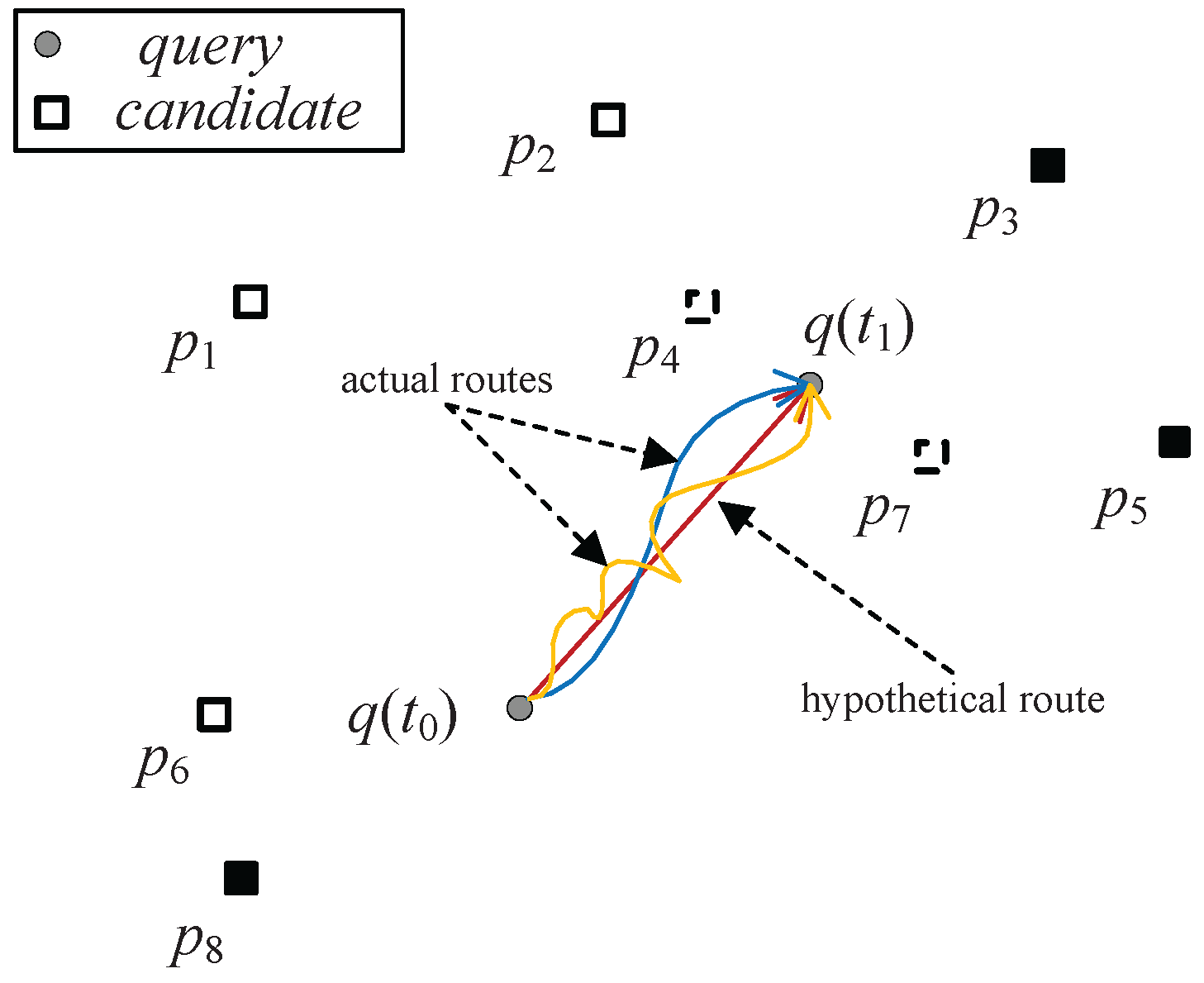
v in at least one dimension. Due to the exponentially increasing usage of smartphones and the availability of inexpensive position locators, location-based services (LBS) are increasingly popular where skyline queries are based on the current location of the user, which changes continuously as the user moves. Taking an example of a tourist looking for restaurants, she/he may be interested in the restaurants close to her/his location that are cheap and have good reputations. Since the distances between the tourist and the restaurants are changing as the tourist travels, the skyline needs to be updated continuously. In addition, the tourist may have a destination in her/his mind and she/he moves towards the place. As shown in
Figure 1, the user at time
(i.e., at the place
) moves in an upright direction (though users may move in arbitrary directions, in reality one user at a time only moves in one direction). At the next time
, the user arrives at the place
. The ideal route may be the red one. However, for various reasons, such as picking up a friend, carriage maintenance, and traffic congestion etc., the actual route may be the yellow or the blue one.
In other real-time applications such as e-games and digital battle systems, the route between a player and her destination may not be straight. Instead, the route is tortuous, as in the routes in the previous restaurant finding example. When the fighting player moves, she should keep her eyes on those guardians who are close and most dangerous to her in terms of energy, weapon, etc. To find suitable restaurants during travel or to escape guardians while moving to the player’s destination, the intuitive approach to updating the skyline query results is to recalculate the skyline results using efficient algorithms from scratch, such as branch-and-bound skyline (BBS) [
3,
4]. However, the relatively effective solution is to cache the last computed skyline results and to only calculate those data objects that may enter or leave the skyline results.
Note that existing approaches always assume that the motion of the query point is continuous and exactly calculable. Huang et al. [
5] assumed that the query point was moving consecutively and the velocity of query point was known as
. Lin et al. [
6] and Guo et al. [
7] considered the motion of the query point a to be a line, and Lin et al. [
6] also assumed the query point was moving within a certain range. For location privacy consideration, the user query point is sometimes assumed to vary in a disk region [
8]. In this paper, we address the motion typically presented incrementally over a series of discrete time steps, which is more practical for real applications.
Since discrete motion patterns are more suitable for moving points, we utilize the incremental motion model for the continuous skyline queries. That is, query points are moving incrementally in discrete time steps. Unlike existing motion models in [
5,
6,
7,
8], given the drift error bound and velocity of the drift, the incremental motion model places no restrictions on the motion or on its predictability (although the direction in this paper is given, we have no restrictions on moving directions). Under the incremental motion model, we utilize the geometric properties to prune the region in which the data objects will not be in the final skyline query results. To avoid calculating the skyline results from scratch while query points are moving, we maintain a data structure similar to kinetic data structures (KDSs) [
9,
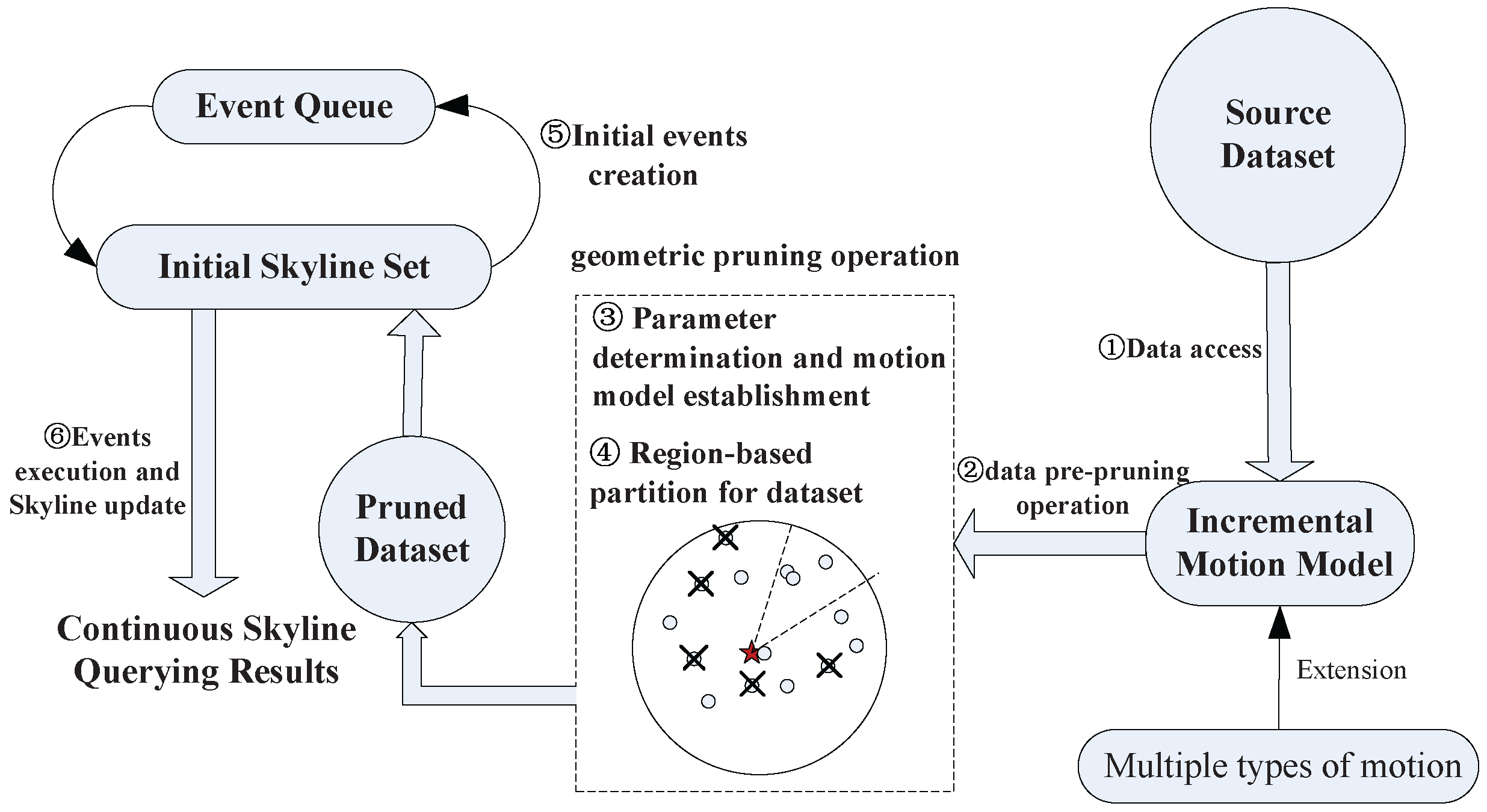
10], which are famous in the area of computational geometry. The KDS keeps the desired relationship between data by storing all those data in some structures specific to the relationship. The contents in KDS do not change unless the relationship between some data points has been changed. The data structure includes a list for skyline query results at each time step. When the query point moves, the data structure decides whether the data object(s) enter(s) the skyline results or goes out of the result set. The implementation of the data structure is based on event-driven mechanisms. The framework of processing continuous skyline queries under an incremental motion model is illustrated as shown in
Figure 2. First, the input dataset is pruned using geometric properties based on the incremental motion model. Then, we calculate the initial skyline results on the pruned dataset. Event-driven mechanisms are adopted to compute the continuous skyline results when the query point is moving. To sum up, the key contributions are as follows:
We adopt an incremental motion model for the continuous skyline queries which neither restricts the motion nor makes any predictions.
By utilizing the geometric properties as a query point moves under incremental motion model, we prune skyline non-result-related data points, which can accelerate the processing of continuous skyline queries.
Instead of accurate dominance, we propose probabilistic dominance under an incremental motion model for two data points which possibly dominate each other. By giving different thresholds of possible dominance, we decide the final query results, which are more actual in real applications.
We demonstrate the efficiency of the geometric pruning strategies under an incremental motion model with extensive experiments on large-scale datasets.
The rest of the paper is organized as follows.
Section 2 introduces related work. Preliminaries are given in
Section 3.
Section 4 presents the geometric pruning strategies. Data structures and event-driven processing mechanisms are provided in
Section 5. Extensions to specific motion patterns are proposed in
Section 6. Results of comprehensive performance studies are discussed in
Section 7.
Section 8 concludes the paper.
2. Related Work
Skyline Queries. The skyline operator was introduced to the database community by Borzsonyi et al. [
1] in 2001. Consequent studies have focused on efficient skyline query processing. Tan et al. [
11] developed bitmap and index techniques. Chomicki et al. [
12] developed the sort-filter-skyline algorithm (SFS), which improved Block Nested Loop (BNL) by pre-sorting the dataset. Several optimizations to the SFS algorithm (e.g., [
13]) increase its efficiency. Kossmann et al. [
14] presented a nearest neighbor algorithm (NN) which allowed users to change preferences during runtime. Papadias et al. [
4] proposed a progressive algorithm called branch-and-bound skyline (BBS), based on a nearest neighbor search technique supported by R-trees. Variations of the skyline operator have also been explored, such as in a distributed environment, road networks, skyline cubes, reverse skylines, and approximate skylines, just to name a few. See [
2] and [
15] for more extensions. However, the above studies only consider static query points on static attributes. Sharifzadeh et al. [
16] first introduced the spatial skyline queries which are also named multi-source skyline queries in road networks by Deng et al. [
17]. They differentiate the attributes of the data objects to two categories: spatial attributes and non-spatial attributes, which are also called dynamic and static dimensions or static attributes and dynamic attributes. They also only considered static query points on dynamic attributes.
Motion Modeling and Skyline Processing. Another related area is monitoring continuous motions using kinetic data structures (KDS) in computational geometry. Basch et al. [
9] first proposed a conceptual framework for KDS to continuously maintain evolving attributes of mobile data. A basic assumption in the KDS framework is that the object trajectories are known. More recently, several efforts have been made to deal with data in much less restricted models of motion. Mount et al. [
18] studied the maintenance of geometric structures in a setting where the trajectories are unknown. They separated the concerns of tracking the points and updating the geometric structure into two modules:
the motion processor (
MP) and
the incremental motion algorithm (
IM). They further presented a simple online model in which two agents named
observer and
builder cooperated to maintain the incremental motion [
19].
Motion considered in skyline queries includes a moving query point and moving data objects. Huang et al. [
5] proposed a kinetic-based data structure to update the skyline results. The query point was moving along with predefined motion patterns (i.e., uniform motion in a straight line). Lee et al. [
20] also studied a similar problem. However, both of the attempts rely on the assumption that the velocities of the moving points are known. Unfortunately, this assumption does not hold in many real-world applications where the points (e.g., cars, tourists) frequently change their motion patterns (e.g., speed and direction). Furthermore, the extension of their techniques is non-trivial for the scenarios where velocities are unknown. Lin et al. [
6] assumed that the query point is in a predefined spatial range instead of an exact location or moving along with a line segment. To handle the movement of the querying objects, the incremental version of the line-based skyline solution has been devised to reduce both the result set size and the computation cost. Hsueh et. al [
21] presented an algorithm to update the skyline when the data objects change their attribute values. Cheema et al. [
22] proposed a safe zone-based approach for monitoring moving skyline queries which allows queries to move in an arbitrary fashion. The query results are required to be updated only when the query leaves its safe zone. In the framework, when a query point moves in the time interval between two adjacent events, its trajectory belongs to a safe zone. Vu et al. [
23] introduced uncertainty both on the query point and Points Of Interest (POIs) for spatial skyline queries. The uncertainties here are represented as square disks with varied radii. Compared to this method, our incremental motion model considers not only the uncertainties (represented by the disk whose radius is the maximum speed), but also the directions. Another difference from these studies is that we prune the data points not belonging to the final skyline results based on geometric properties as a preprocessing step, which accesses less data points and thus saves more CPU time. The authors in [
3,
4,
24,
25,
26] studied dynamic skylines. However, [
3,
4,
24] used branch and bound method (BBS) to calculate the skyline results from scratch. References [
25,
26] utilized a caching mechanism to accelerate the dynamic/constraint skyline query processing. However, for continuous skyline queries, they are based on past queries not fully utilizing the query results of last moment. In addition, the methods of Sacharidis et al. [
25] are not practical due to the shortcomings of bitmap coding mechanisms.
3. Preliminaries
When query points move, the distances between the query point and data points need to be estimated for further processing of skyline queries. In this section, we first estimate the location of the query point on incremental motion model, and then evaluate distance dominance between the data points for further calculating skyline results.
Table 1 summarizes the notations frequently used throughout the paper.
3.1. Problem Definition
Given n data points in the dataset , each point has d-dimensional non-spatial attributes, also called static attributes. Each point is stored as , and , are the location of and jth-dimensional static attribute of , respectively. Thus, can be represented as , where is the distance of the query point q and data point .
Definition 1. (Static Dominance) For two data points and all attributes of except distance attribute, , and at least one < holds, we say that statically dominates , represented as .
Definition 2. (Complete Dominance) For two data points , , and at least one < holds, we say that completely dominates , denoted as .
Although the skyline processing involves spatial and static attributes in our problem, some data points could be always in the skyline no matter how the query point moves. This is because these data points have the dominating nonspatial attributes which guarantee that no other data points can dominate them. We denote this subset of skyline points as , the final skyline query results as , and the difference of the two sets , as for data points in might not be skyline points when query point moves. It is obvious that contains two parts: the first part is , which includes the data points from non-skyline dataset . These points become skyline points when the query point moves. The second part is , which contains the skyline points not moving out of when the query point moves.
Instead of snapshot skyline queries like I/O optimal BBS method, we define the continuous skyline queries as follows.
Definition 3. (Continuous skyline queries) Given the skyline results at time , the skyline result at next time is based on and only considers two varied sets: , the data points move out of skyline results of time , and , the data points from become skyline points.
From References [
1,
5,
20,
21], we know that the skyline result
is small compared with
. However, the dataset
is also too large. Fortunately, not all data points in this dataset have the possibility to become skyline points. In practice, according to the motion of query point
q, only a very small part of
can be skyline points. So, the computation overhead of the continuous skyline queries will be decreased to some extent compared with snapshot skyline queries.
3.2. Incremental Motion Model
The incremental motion model was first proposed by Mount et al. [
18]. Later, Cho et al. [
19] utilized this model to maintain net and net tree structures under an incremental motion model. We give a brief introduction to this model with adaptive modifications to our problem.
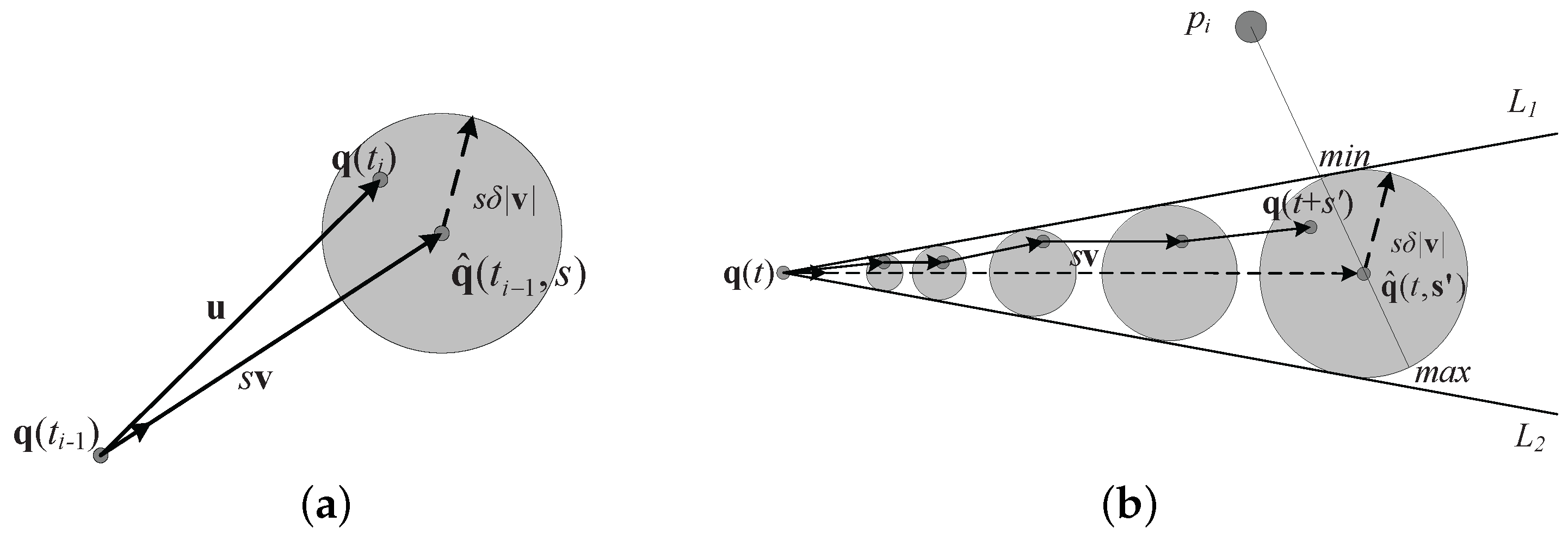
3.2.1. Query Point Position
Let
q be a query point. The position of
q in Euclidean space at time
t is denoted as
. The motion of point
q,
, is a finite sequence of point positions sampled at discrete time instances:
, where
. The interval between two consecutive instances is a time step:
. Let
v denote the estimation of a query point’s current velocity. The estimated displacement of the point over this step is
, and its actual displacement is given by the vector
. Let
denote the Euclidean length of vector
. we use drift of this point at time
to represent the relative error between the actual and estimated displacements:
Let
δ be the drift bound; we say that the motion
satisfies this motion estimate if for all time steps the drift of
relative to the velocity estimate
v is at most
δ. Given the velocity estimate
v and given any time
t, the estimated location of the point after an elapsed time of
s is defined to be
. For example, the estimated location of
after step
s is
(see
Figure 3a). Let
denote a Euclidean ball of radius
r centered at point
q. From the above definitions, we have
Let
T be a time interval of duration starting at time
t,
. If a motion
satisfies a given motion estimation, then for each time instance
,
, the query point
lies within a Euclidean ball centered at
and the boundary of
is determined by a series of the balls mentioned above (see
Figure 3b). The following equation specifies the constraints on its position at any time:
3.2.2. Time Parameterized Distance Function
In our problem, the velocity of a query point is determined by the positions of the point at different time steps:
For simplicity, we assume that the query point
q moves in 2
d space,
, and the position of
q at time
is
. We use
to represent the center of the Euclidean ball. At time
,
. After an elapsed time of
, the center of the incremental motion model
changes to
and equals to
. Then, for a data point
p located at
, at time
, the estimated distance between
and
p can be expressed as follows:
By Equation (
3), the estimated location of the query point is
. Since the estimated location of a query point after an elapsed time
s is in a Euclidean ball, the actual distance between
and
p is constrained in a certain range (see
Figure 3b). We use
to denote the distance between
p and
:
Besides,
is used to denote the actual distance between
p and
, which is in the range of
denoted by Equation (
6).
3.3. The Dominance Relationship of Distance
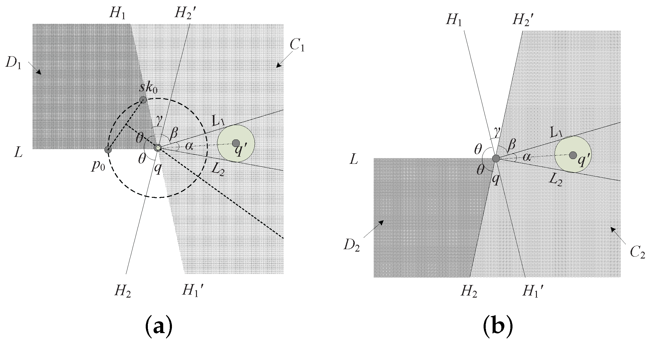
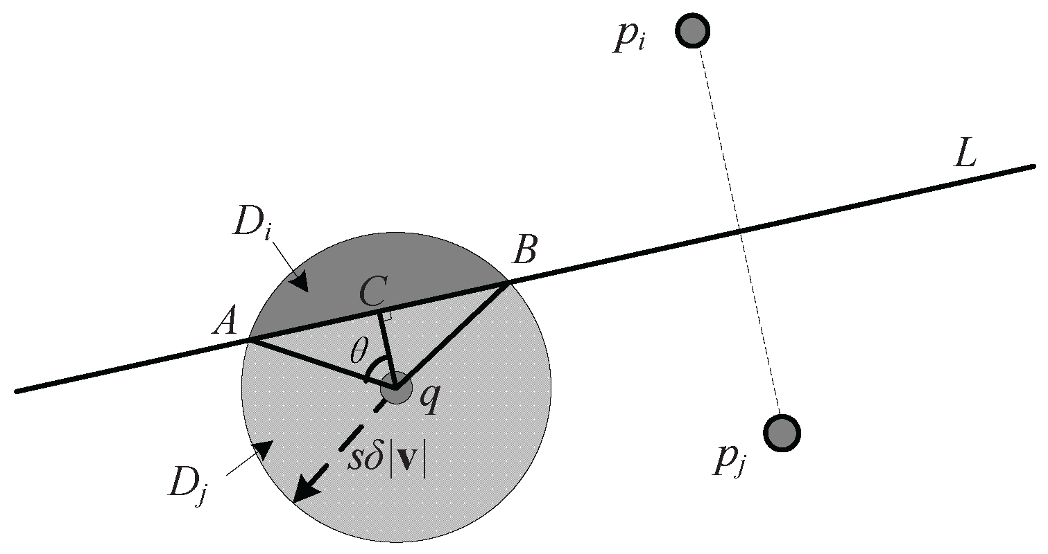
As the query point moves constantly, the distance between the moving point and each data point changes, which is inaccurate because we cannot predict the actual position of the query point exactly. However, we are sure that the distance is in a certain range: . In addition, if , is closer to the query point than . The dominance relationship between and is not confirmed, because both of them are inaccurate but within a known range. So, we need a rational method to compute the probability that is better than in distance.
Assume that after an elapsed time
s, the position of a query point is shown in
Figure 4, the radius of the incremental motion model is
, and
L denotes the perpendicular bisector of
which divides the ball into two regions:
and
. Then, we use
A and
B to denote the two intersections of
L and the ball. When the query point
q is within region
,
.
Lemma 1. Assume that the position of query point q is uniformly distributed in the Euclidean ball. The angle between the estimated position of query point q to the intersections of the perpendicular bisector of and the bound of the incremental motion model is , then the probability that is better than in distance, denoted by , can be calculated by Proof. As long as the query point is in the region , is closer to the query point than ; consequently, the probability that is better than in distance is equal to the probability that the query point falls in the region . Assuming that the possible positions of the query point are uniformly distributed in the ball, we only need to compute the proportion of region to the whole ball.
The angle between the estimated position of query point
q to the intersections of the perpendicular bisector of
is
, so the area of fan-shaped AqB is:
where
R denotes the radius of the ball.
In addition, the area of triangle ABq is:
So, the area of
can be expressed as follows:
Then, we can obtain that:
☐
From the above analysis we can see that with the movement of a query point the distance between the moving point and each data point is not certain, and is related to the estimated position of the query point. Next, we will give the definition of dominance in distance. Lemma 1 has shown how to compute the probability that is better than in distance.
Definition 4. (Dominance in Distance) If the probability that is better than in distance is greater than a predefined threshold—That is, —, we say that dominates in distance (i.e., ).
Definition 5. (Skylines based on Thresholds) If or , and cannot dominate each other in distance, and if no other data point can dominate or , they both belong to the skylines.
The probability here is defined by the ratio of two areas (see
Figure 4 and Equation (
11)); the skyline queries are not probabilistic skyline queries as in Pei et al. [
27] where probabilities denote the probable occurrence of each possible world from the PWS (possible world semantics) space composed by uncertain data objects.
5. Skyline Computation
5.1. Continuous Skyline Query Processing
We now explore the continuous skyline query processing techniques according to the above analysis. A naive way is to call the existing algorithms to process skyline queries in each time step to acquire continuous query results. Since we know the estimated position of the query point and parameters of the associated incremental motion model, the results are credible. However, processing continuous skyline queries in this way needs to traverse the entire dataset repeatedly, which will inevitably increase the running time and I/Os. In practice, the speed of a query point is not very fast; therefore, the skyline will not change frequently. For example, as mentioned in
Section 1, a user is looking for restaurants. Her/his moving speed is considerable not too fast. So, the skyline results in the last moment can be utilized to process skyline queries of the next moment. Otherwise, if the speed is too fast or the time interval is large enough that the skyline results in the last time step are all changed at the next moment, we would rather utilize snapshot skyline queries for this situation. For the motivation examples, these will not occur. So, in this paper, we assume the query points are not moving too fast and skyline results in last moment can be used for next time step query processing. For the problem, we can use the strategies mentioned in previous sections to compute the intersections that may influence the skyline and maintain the skyline results incrementally.
First, we compute the initial skyline. After that, we decide which moment may cause the skyline change and record the intersections the skyline results may change. Then, when an intersection comes, we deal with it and determine further intersections for the updates of the skyline.
Corollary 1. Assume that the distances of skyline points , , and to the estimated query point is an increasing sequence, then the intersection between and will not occur before an intersection between any two adjacent points of , , and .
Proof. Assume that and intersect at time , , , and , intersect at time , , respectively. Before an intersection, we know that , and we only need to prove that must be later than and . Now suppose that is earlier than or . So, after time , . Additionally, is still valid since no intersection happens between any two adjacent points, which contradicts . Therefore, must be later than and . ☐
We stored the skyline in a sequence according to their distances to the query point. We also only need to compute intersections between two adjacent skyline points.
5.2. Data Structure and Conditions
We use a bidirectional linked list (other similar data structures, such as heap and array are also fine for we process these structures not “on-line”; instead, they could be processed during the interval of two time steps) named to store current skyline points, which are sorted in ascending order of their distances to the query point. The form of each skyline point in is denoted as . indicates whether belongs to , is the distance between and the query point q, is the validity time of , which is only available to each changing skyline point and recording the time when is dominated, and is the time will exchange its position with its successor in (see the algorithms below for details).
By Theorem 2, there are two situations that may cause the skyline to change. Assume the time of an intersection is
(
):
Before time , is a changing skyline point. is farther to query point q than , and dominates in all static dimensions. Then, after , will be dominated by and leave the skyline;
Before time , is a skyline point, and is a nonskyline point. Then, after , can enter the skyline depending on whether is the unique skyline point which dominates it.
To summarize the above analysis, we only need to consider the cases which may cause the skyline to change. For simplicity, this paper has made two assumptions on the threshold
τ:
The perpendicular bisector of
goes through the centre of the ball in the incremental motion model, so
, we can derive from Lemma 1 that:
For
, before time
,
, and after that
(as shown in
Figure 8).
Assume that the perpendicular bisector of
goes through the point
C where is 1/4 of the diameter (see
Figure 4); i.e.,
. Therefore,
, and
; we can obtain from Lemma 1 that:
For convenience of calculation, we set
.
Theorem 3. As shown in Figure 8, assume that the position coordinates of , are and . The query point is starting from with velocity , then the time of the intersection can be presented as below:- 1.
,
- 2.
, time of the intersection are and , and can be given as follows: , where , .
Proof. The coordinates of
,
are
and
, the perpendicular bisector of
, denoted by
L, can be written as:
; that is,
. Let
,
:
If , we only need to compute when the query point will meet the perpendicular bisector of ; that is, the moment and is equal to the distance to the query point: , then
If
, at time
and
, the query point satisfies the condition of 1/4 of the diameter (see
Figure 4) , time
and
are the tangential moments of the perpendicular bisector and the bound of the ball in the incremental motion model. We derive time
via
and
;
is similar. The vertical speed of the perpendicular bisector is denoted by
. At time
, distance from the query point to
L is equal to the current radius of the ball in the motion model, so we have
. According to (1),
, then
can be obtained by
. Therefore, from
to
, the distance varies along the direction of
is equal to half of the radius. So,
.
Based on the above equations, as a conclusion,
. Similarly,
. ☐
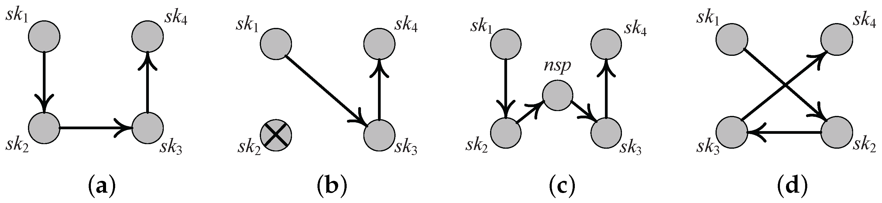
As the query point moves, the distances between all data points and the query point are varying, which may cause the skyline to change. According to the type of the change, three events are formulated as follows:
Event . This occurs when any skyline point leaves the skyline, which will only happen to a volatile skyline. Assume that , and there is another skyline point with potential to dominate , then if intersects with in distance and , will leave the skyline; that is, an event happens.
Event . This occurs when any nonskyline point enters the skyline. For a nonskyline point and all those skyline points currently dominating it, if gets closer to query point q than skyline point , can no longer dominate it; that is, an event happens. However, whether it will enter the skyline depends on whether is the only one to dominate it. This will be checked when an event of this kind is being processed.
Event . This occurs when a couple of skyline points in make a sequential change. For a skyline point , if it intersects with its successor and cannot dominate it, and exchange positions in ; that is, a event happens. Notice that does not have the potential to dominate ; otherwise, an event will happen instead.
As shown in
Figure 9, the list includes
data points, and the points are sorted in ascending order of their distances to the query point. At time
t,
,
dominates
in all static dimensions. Then, an
event will happen because
will be dominated and leaves the skyline (see
Figure 9b). If
is the skyline point dominated by
uniquely, at time
t, if
, then an
event will happen because
will enter the skyline (see
Figure 9c). Additionally, at time
t, if
gets closer to query point
q than
and
has no potential to dominate
, then an
event will happen because
and
will exchange their positions in the list (see
Figure 9d).
A global queue is used to maintain all events to represent future skyline changes. Each event is in the form of when the event happens at time , and is used to record the kind of this event. and respectively represent the skyline point and the relevant data point involved in the event. In an or event, represents the skyline point , while is its successor . In an event, represents the skyline point while stands for the relevant nonskyline point .
Initially, contains all the current skyline points while Q contains recent events that will happen in the nearest future. As time elapses, events in the queue are dequeued and handled according to their types. While handing events and updating the skyline, the process also incurs future incoming events. Therefore, Q evolves with existing events being dequeued and new events enqueued. After all due events are processed, contains all the correct skyline points with respect to the query point q’s current position.
5.3. Event-Driven Mechanisms for Continuous Query Processing
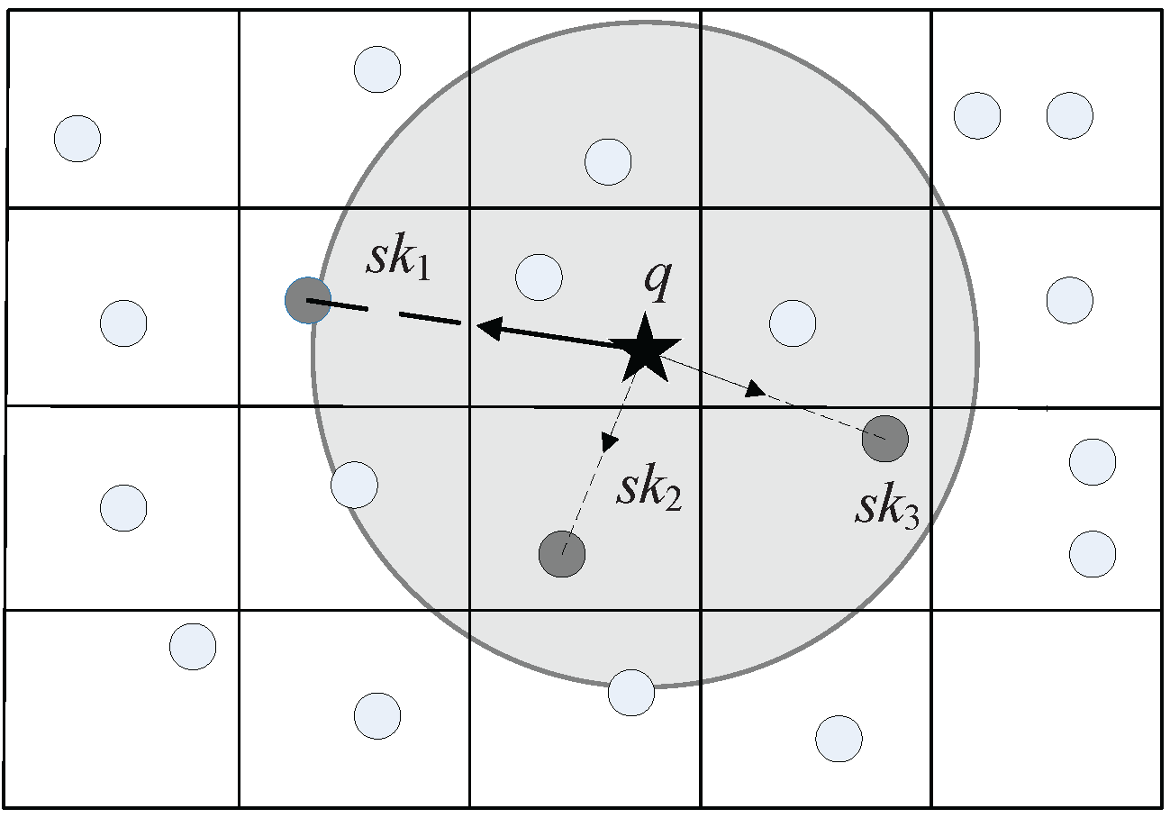
In our method for the static data set, we use a simple 2D
grid file index dividing the data space into
cells. We set the data points within each cell are stored in one disk page. At the beginning of the algorithm, the static skyline will be computed in advance. According to Lemma 2, the farthest distance is recorded in variable
as a search bound, and the cells beyond
are pruned for reducing I/Os (see
Figure 10).
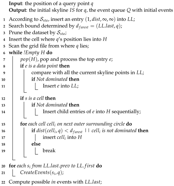
As shown in Algorithm 1, in initial, all permanent skyline points in
are inserted into
based on their distance to the starting position of query point
q. First, we prune the dataset by utilizing geometric properties. Then, starting from the cell where
q’s initial position lies, all grid cells are searched in a spiral manner so that those on an inner surrounding circle are searched before those on an outer one, as shown in
Figure 10. Then, we organize the data set according to Lemma 3, 4, 5 with heap structure. A heap
H is used to store cells or data points that are possible to enter the skyline, which its top is the cell or the data point which is closest to
q’s estimated position. Points or cells in the heap are sequentially compared to the current skyline points in
, which is adjusted with deletion or insertion if necessary. After that, events will be created for continuous skyline query—all events for all skyline points, except the last one in
. Next, the farthest skyline point is applied to compute possible
events for those points farther than it.
| Algorithm 1: Initialization |
![Ijgi 06 00091 i001]() |
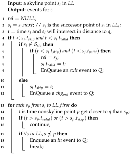
Algorithm 2 has shown the process of CreateEvents in detail. For a given skyline point , the algorithm first computes the time t when and the next skyline point in will exchange their positions in the list that will dominate in distance. If t is later than ’s exchange time or ’s validity time, it is ignored. Otherwise, it means an event depending on ’s validity time if , or it is a simple event. Then compute events for each nonskyline point that distance to q’s estimated position comparing with and ’s distances.
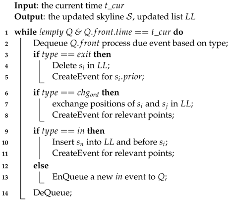
When the nearest event in Q happens, it is dequeued and processed with the relevant points involved according to its type. Then create new events after the new skyline is obtained (as shown in Algorithm 3). At any time when Q is empty, all the points in are the correct skyline of the current time point.
According to Algorithm 3, the actions to process each kind of event are described as follows: for an exit event, is removed from the skyline list and creates new events for its predecessor since the successor has been changed; for an event, the nonskyline point will be checked to see whether it is unique and dominated by . If yes, will be inserted into the skyline list and new events are computed for relevant points. Otherwise, a possible new event is computed and enqueued. For a event, the skyline list is correctly adjusted by exchanging the positions of and . Similarly, relevant events are created and enqueued for them and their predecessors if exists.
| Algorithm 2: CreateEvents |
![Ijgi 06 00091 i002]() |
| Algorithm 3: Process due event |
![Ijgi 06 00091 i003]() |
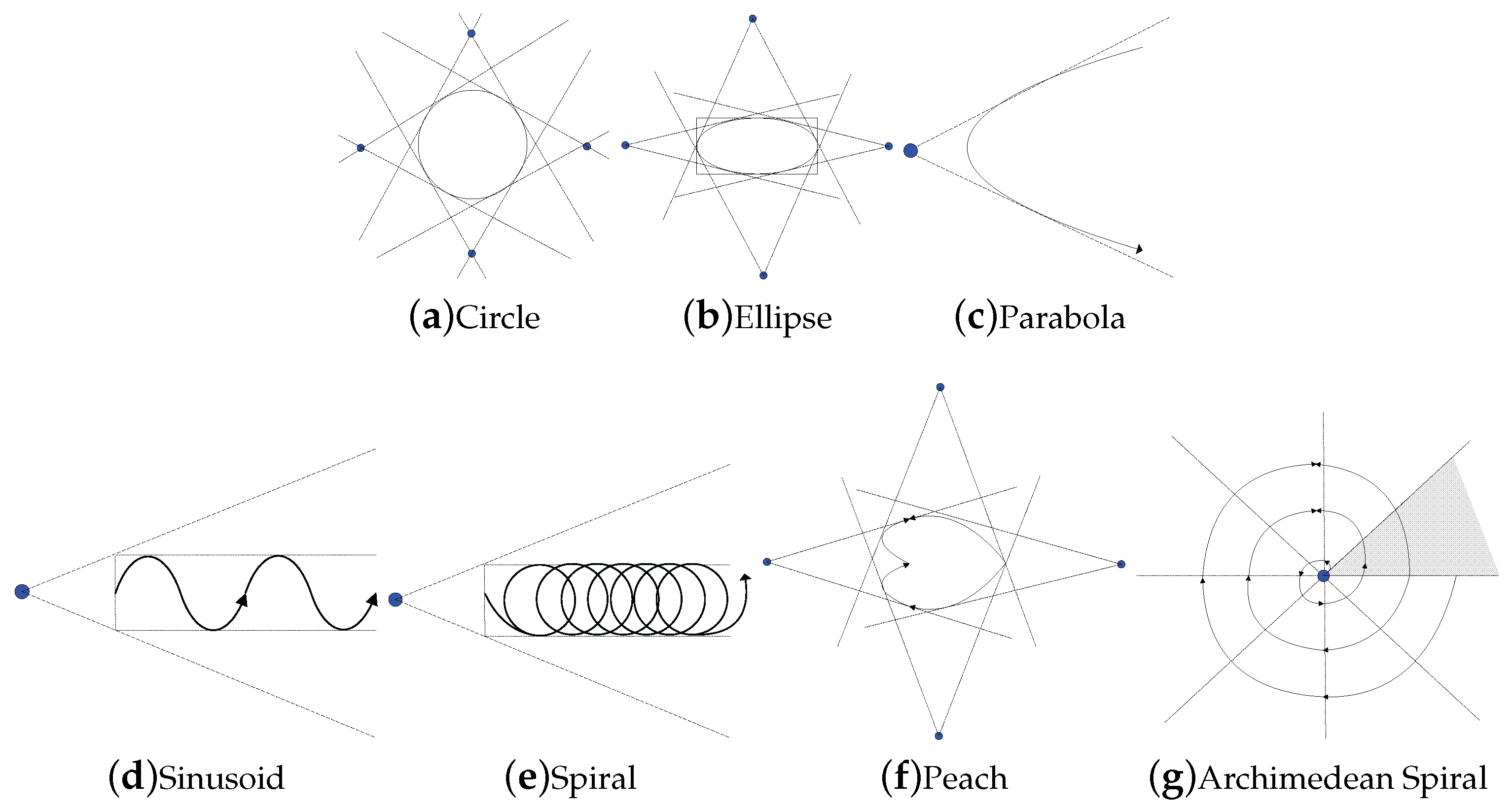
6. Pruning Strategies for Specific Motion Patterns
The geometric pruning strategies can be easily integrated into the known moving trajectories to reduce the number of data points. In this section, we provide the geometric pruning strategies under the incremental motion model for three different classes of trajectories: enclosed, bounded, and unbounded. In the case that the movement or part of the moving range boundary of a query point is known, if the position of the point is now not qualified to establish an incremental motion model, we assume that there is a “virtual query point” somewhere in the past, and it was able to be applied to the incremental model. Moreover, the movement of the true query point—though not consistent with the incremental motion model—stays in the estimated region of the incremental motion model set up by the virtual query point.
Enclosed motion patterns If the movement of a query point
q is an enclosed curve, the query point stays in the enclosed region surrounded by the curve.
Figure 11a–c are three typical enclosed motion patterns:
circle,
ellipse, and
parabola. In this case, in spite of
q’s moving speed, the point moves along the curve and makes an influence to the skyline repeatedly. In consideration of the characteristics of enclosed curves, the exact upper and lower bounds in all directions of a query point can be obtained. Based on all of the above curves, we can establish incremental motion models in different directions to acquire a series of virtual query points; after that, the geometric pruning algorithm will be executed iteratively, and filtering out most of the redundant points which make no influence to the skyline.
Motion patterns with bounds If the movement of a query point
q is a curve with bounds, it means that we can acquire its upper and lower bounds in one or several directions while the rest have no boundaries or could not be predicted (
Sinusoid and
Spiral are two of this kind of motion pattern, as shown in
Figure 11d,e). According to the property of these curves, we can still utilize the starting position of the query point and the directions that bounds can be obtained to establish an incremental motion model, get a virtual point, and apply to the geometric pruning strategies. Basically, though the effect of filtering is not as efficient as the situation of enclosed patterns, it is still worth executing compared to snapshot skyline queries.
Motion patterns without bounds If the movement of a query point
q is a curve without bounds, then no bounds can be gained in each direction and it is infeasible to use the geometric pruning strategies based on incremental motion model (examples of this kind of motion pattern are
peach and
Archimedean spiral in
Figure 11f,g).
According to the characteristics of different types of trajectories, the curves can be classified as follows:
There exists an upper or lower bound in one or several directions (prerequisite). For this kind of curve we can try to establish an incremental motion model by making a pair of tangent lines (e.g.,
parabola,
logarithmic curves). The qualifications of tangent lines are:
- (a)
There exists an upper or lower bound in some direction(s).
- (b)
The pair of tangent lines will intersect and generate a virtual query point.
- (c)
The angle between the pair of tangent lines satisfies the demands of the geometric pruning framework.
There exists no bound in all directions or it is unable to acquire a pair of qualified tangent lines in (1). In this case, we cannot adopt the geometric pruning strategies directly. Then, we need to take the characteristics of the curves into account and adapt it to the framework by adding additional restrictions.
7. Experiments
A n
ive approach to monitoring moving skylines is to call existing algorithms such as I/O optimal BBS [
3,
4] to recompute the skyline whenever the results need to be updated. In this section, we compare the n
ive algorithms to the proposed methods against various factors which may potentially affect the performance of the algorithms. All the algorithms are implemented in standard C++ with STL library support and compiled with GNU GCC 4.9.3. Experiments were run on a PC with Intel Core i3-3240 3.40GHz dual CPU and 4G memory running Ubuntu Linux 14.04 LTS. The disk page size was fixed to 4096 bytes.
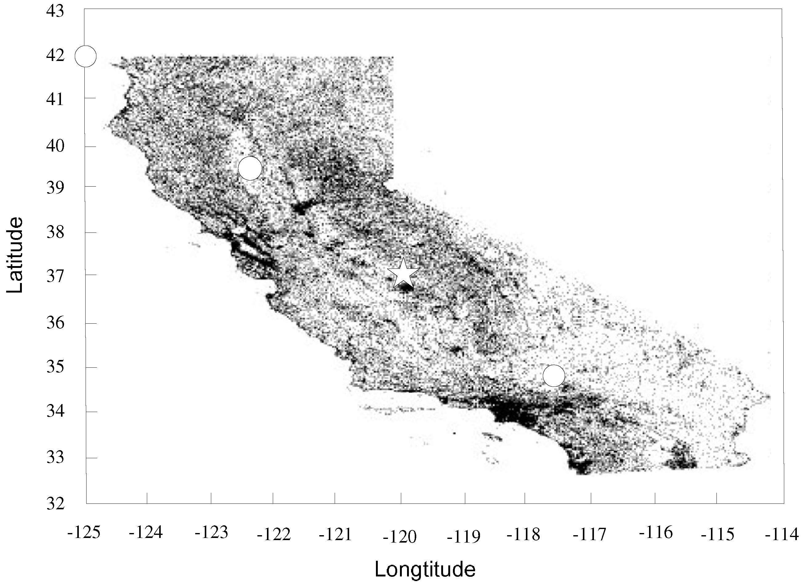
To generate datasets for the experiments, we first fetched real-life California’s interesting points from the website [
28] (see
Figure 12), then we combined the real locations with nonspatial dimensions following different distributions: Independent, Correlated, Anti-correlated, and Zipf. The data size of California’s real locations is about 100 K, and we generate nonspatial dimensions like that in reference [
1]. The attribute value of a data point varied from 1 to 1000. CPU time and I/O counts were used to measure the efficiency of the algorithms under 100 runs of skyline queries. The concerned parameters used in the experiments are listed in
Table 3. In particular, the following algorithms were evaluated:
Continuous skyline query (CSQ): Incremental model-based continuous skyline method which performs the skyline change tracing algorithm in reference [
5] directly without using the geometric pruning strategies.
GP-CSQ: Method performing the skyline change tracing algorithm combined with the geometric pruning strategies using the Lemma 3 (Lemma 4, its extension) only.
GP2-CSQ: An instance of the method performing the skyline change tracing algorithm combined with the geometric pruning strategies using both Lemma 3 (Lemma 4) and 5.
Since the BBS algorithm is the most efficient method for computing skyline in static settings (both data points and query point are static), we adopted it for comparison in the experiments. When the location of the query point changed, we only modified the “
mindist” to adapt the basic BBS algorithm (see [
4]). Besides, we also used the method which is called “ex-BBS” in [
5] for contrast to our proposed methods.
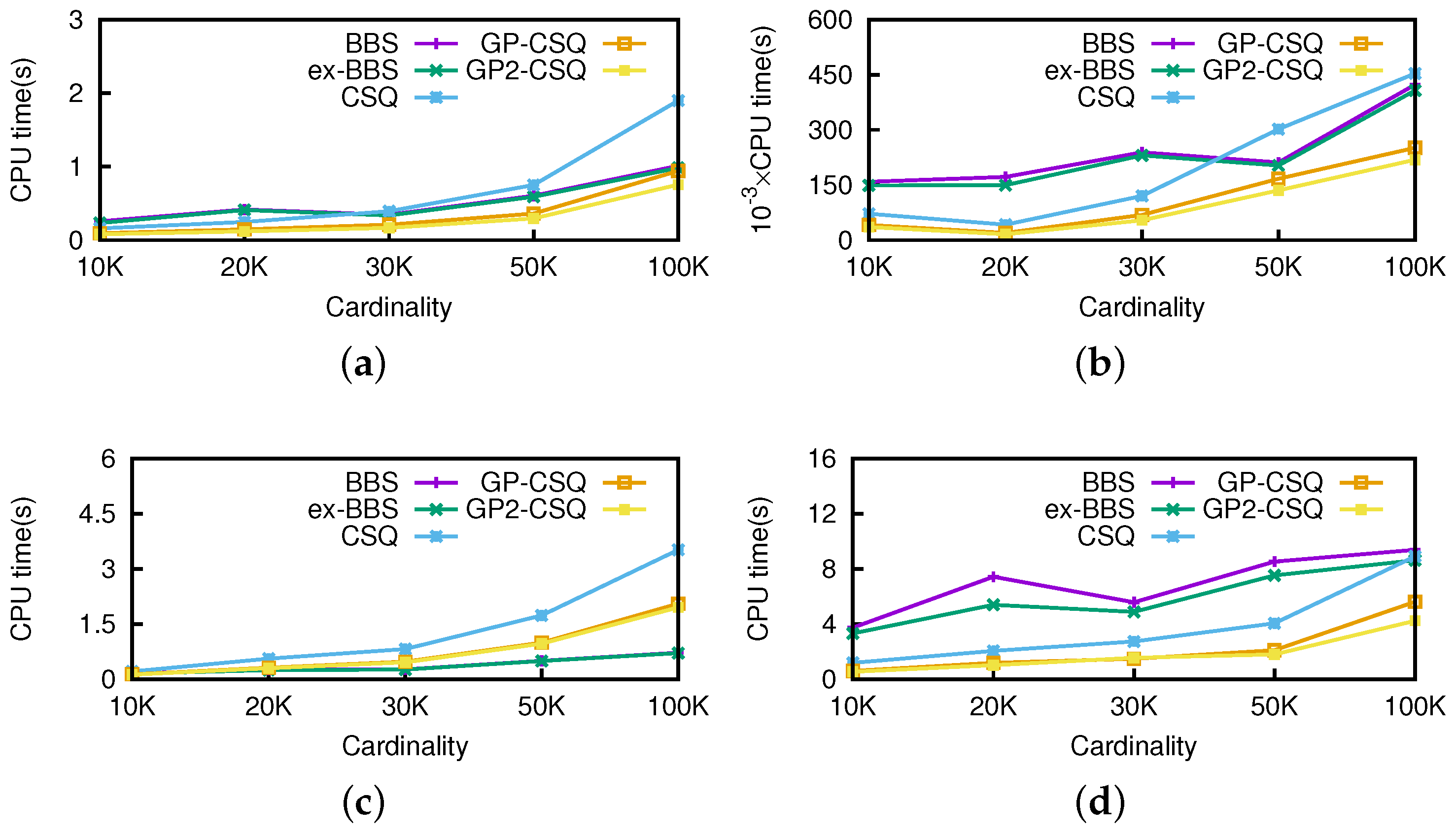
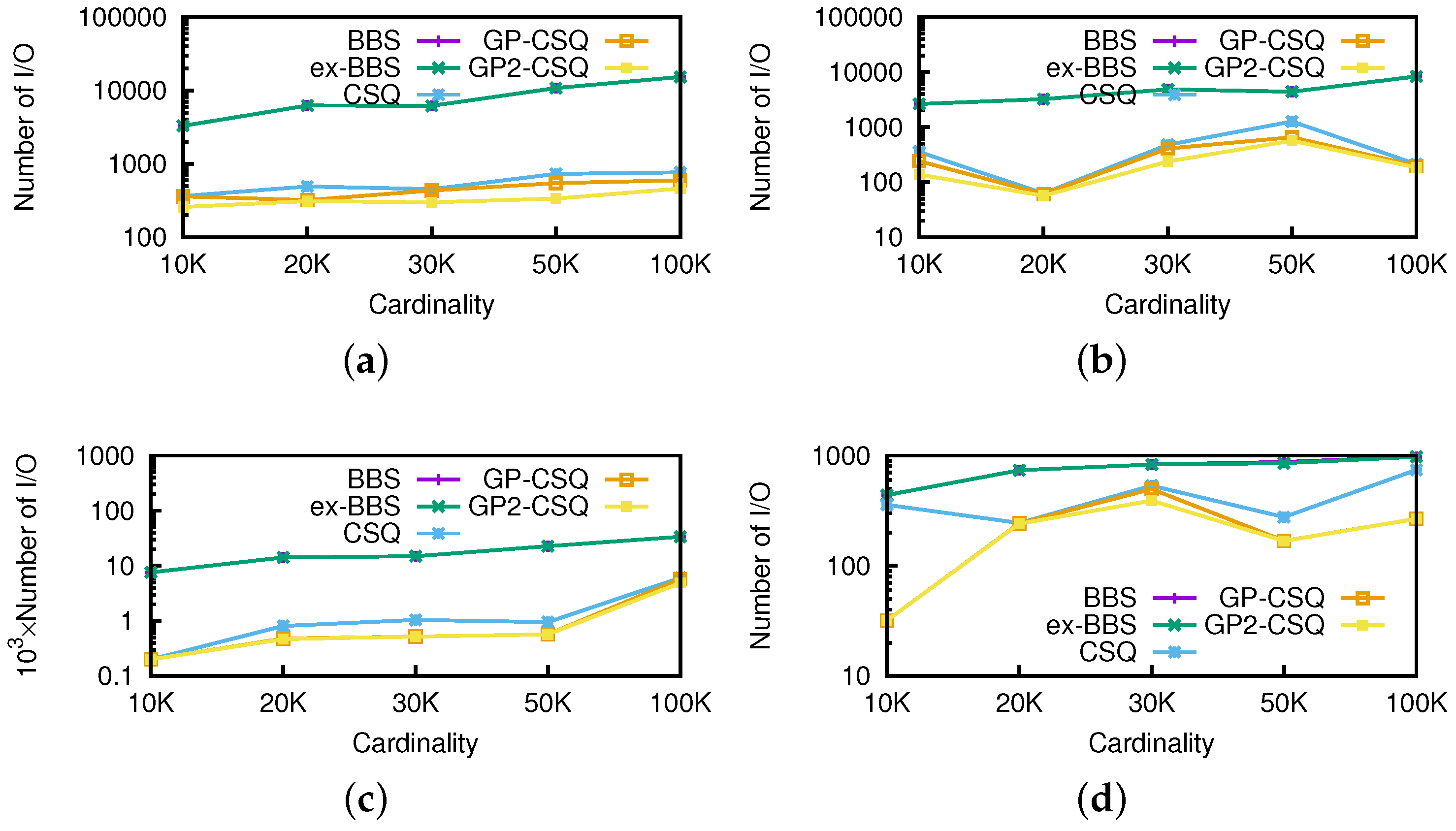
Effect of Cardinality. To generate different-sized datasets, we randomly selected part of the real locations and then combined with two synthetic nonspatial dimensions. Thus, we converted the size of the datasets from 10 K to 100 K. Then, we executed 100 (10 for anti-correlated) continuous skyline queries on the datasets. For each query, we set the starting position of the query point as (37 N,−120 W). The default speed of the query point was (1, −1), while the moving direction was the same as vector (1, −1). The threshold was fixed to be 0.5.
In
Figure 13, the CPU cost of the original CSQ algorithm is higher than BBS algorithms in some cases, because CSQ not only processes non-skyline objects but also computes the initial events to maintain the skyline in the future; GP-CSQ and GP2-CSQ were faster in general because the geometric pruning policies can filter out a large number of unqualified data points and cut down the CPU cost of event computing. Note that in
Figure 13d, CSQ takes much time and the size of the skyline results is large because anti-correlated datasets incur more events.
Figure 14 shows that as cardinality increases, the I/Os of CSQ, GP-CSQ, and GP2-CSQ are nearly 10% less than that of BBS, while GP-CSQ and GP2-CSQ are a little better than CSQ algorithm.
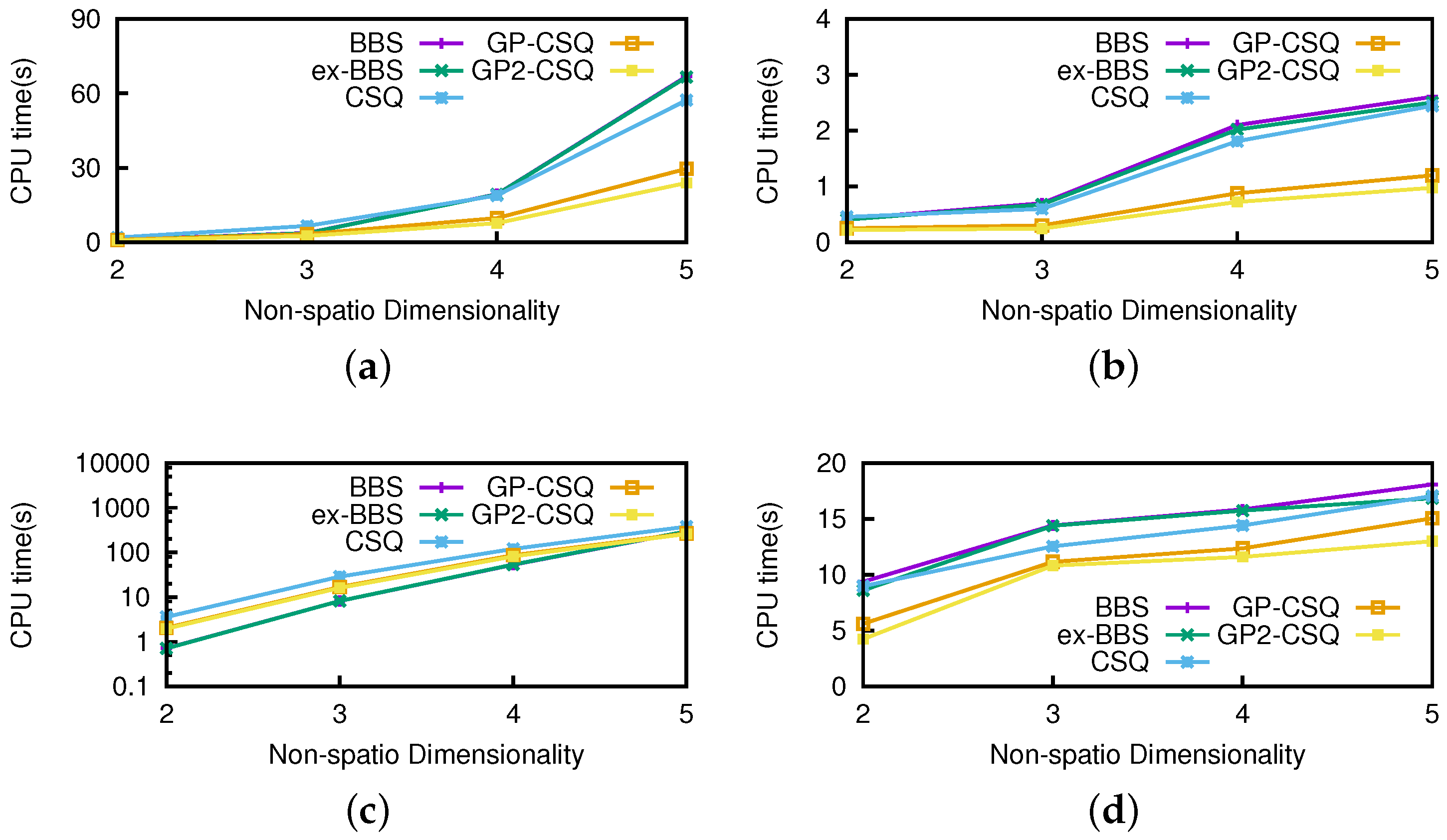
Effect of nonspatial dimensionality. We used a real 100 K road network dataset combined with nonspatial dimensionality ranging from two to five to evaluate the effect of nonspatial dimensionality on our methods. Values on these nonspatial dimensionalities varied from 1 to 1000. The set of other parameters are the same as shown in
Table 3.
As shown in
Figure 15, the pruning strategies can save running time to a certain extent while supporting higher nonspatial dimensionality. In
Figure 16, CSQ algorithms have a clear advantage in I/Os since they focus on dynamic attributes while nonspatial attributes are considered only in dominance checking. Note that the efficiency of the geometric pruning strategies were affected slightly because a data point is harder to be dominated in higher nonspatial dimensionality and makes it almost impossible to prune more data points.
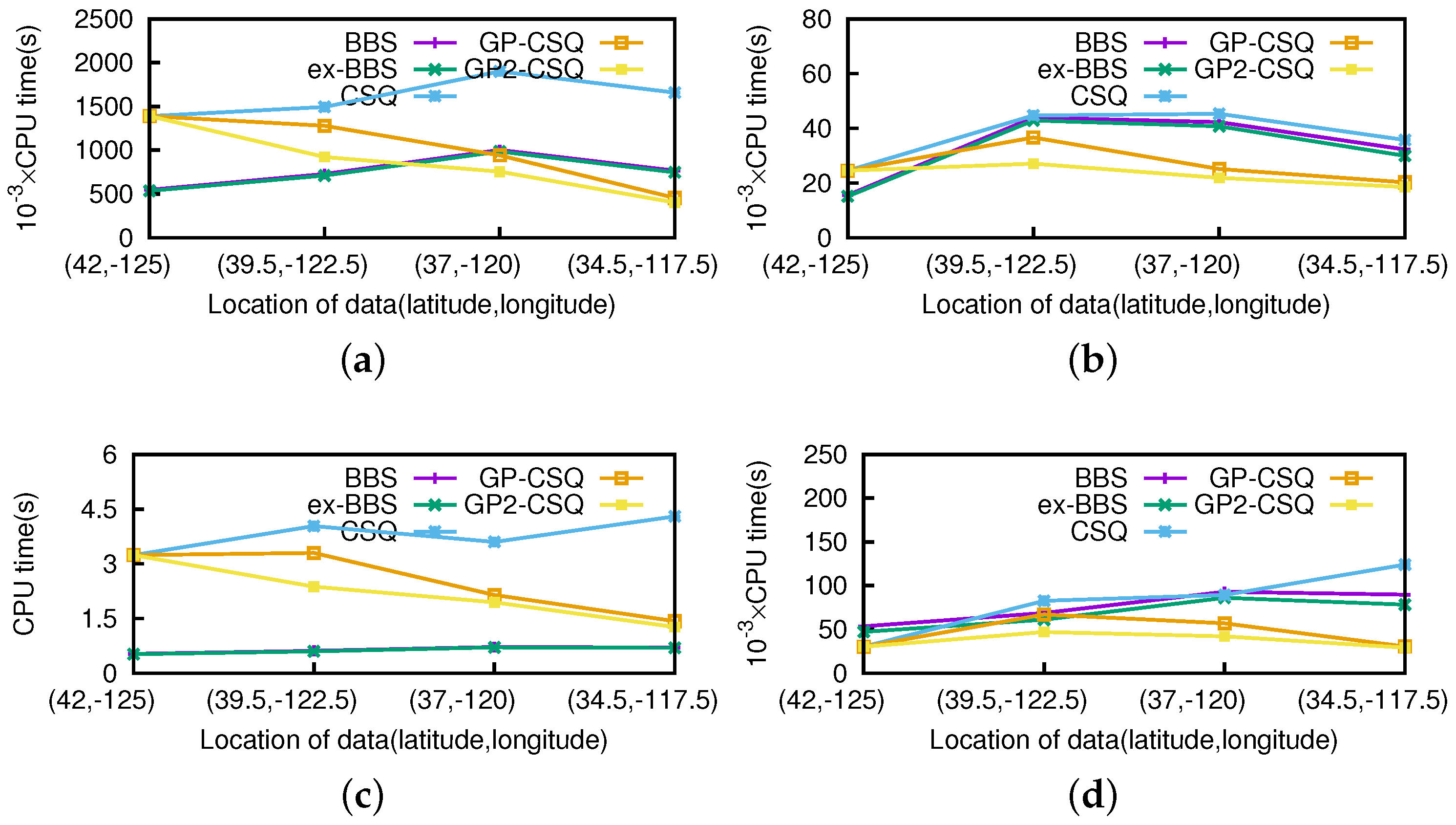
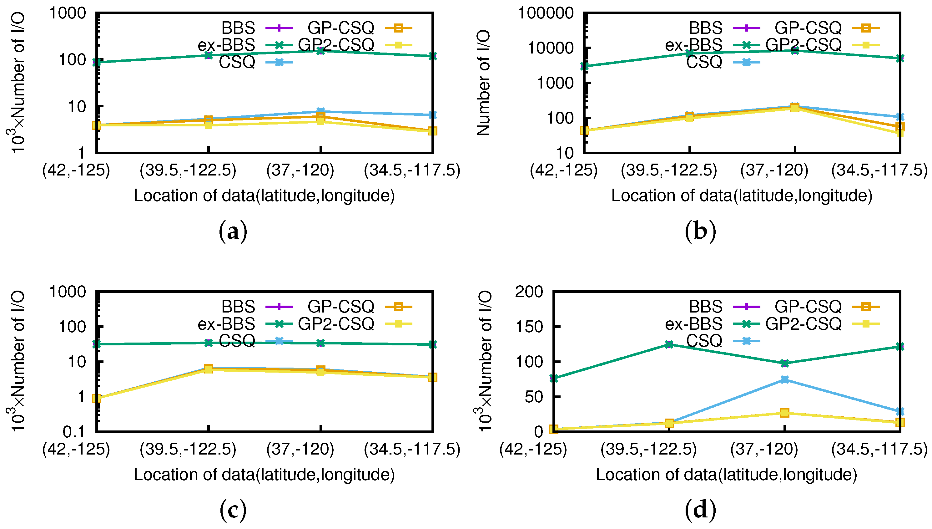
Effect of Starting Positions. Obviously, the effectiveness of geometric pruning strategies is related to the location of query points. In this section, we performed experiments simulating an object moving from the northwest to the southeast in California to verify the influence of different starting positions. Representatively, the starting positions will be chosen in (42 N,−125 W), (39.5 N,−122.5 W), (37 N,−120 W), (34.5 N,−117.5 W); other query parameters were picked up in the same way as in previous experiments. We mainly explored the effect of position related to the efficiency of the pruning strategies by choosing the above four representative positions for evaluation. Moreover, we intended to obtain the general performance of the geometric pruning strategies.
As shown in
Figure 17 and
Figure 18, the costs are quite distinct since the efficiency of pruning operations are obviously affected by the positions of the query point. The pruning operation of ex-BBS was almost disabled since there exists a permanent skyline far from the query position. If the query point approaches the center of the spatial area, the pruning operations of ex-BBS are more likely to malfunction. The geometric pruning strategies tend to be available except in the extreme situation in which the query point is starting from the edge of the spatial location. Moreover, the proposed GP-CSQ and GP2-CSQ methods can filter out most of the unqualified data points in some specific cases in which the region to be pruned is extensive (e.g., in the position (34.5
N, −117.5
W), saving about 60%–80% of CPU time and I/Os). Note that in
Figure 17d, the CPU cost of the CSQ algorithm is much higher since there are a mount of events needing to be computed and GP-CSQ and GP2-CSQ are approaching that of BBS due to the optimization of the geometric pruning strategies.
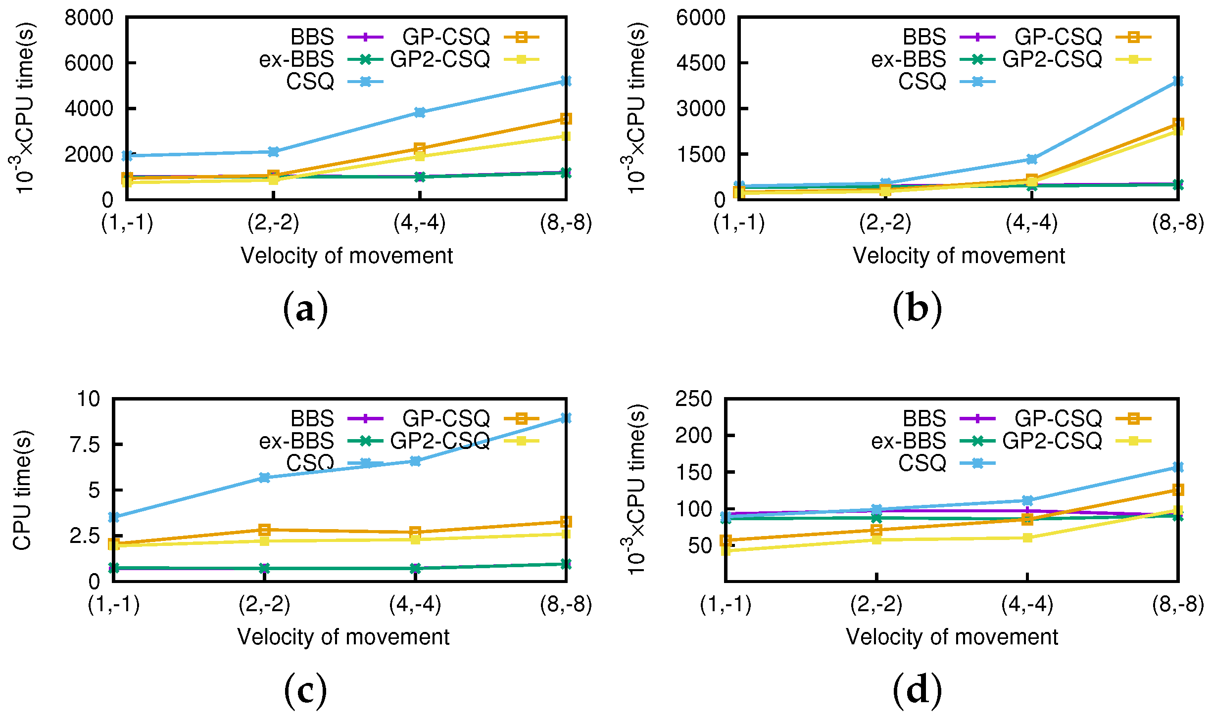
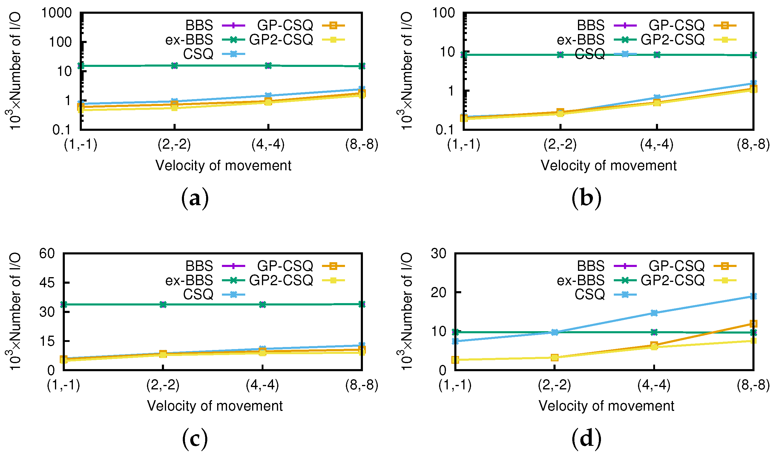
Effect of Moving Speed. In this section, we run the experiments where the speed of the query point varies from (1,−1) to (8,−8). We still use the real-world dataset of 100 K combined with two correlated, independent, anti-correlated, and zipf-distributed nonspatial attributes.
In
Figure 19 and
Figure 20, it is obvious that the cost of CSQ increases with the query speed because the distance of data points intersects more frequently, which means larger numbers of events incur and need to be disposed of, thus consuming more I/Os and CPU time. Optimized by the proposed geometric pruning strategies, the I/O cost of GP-CSQ and GP2-CSQ is not too sensitive. However, the CPU time for creating and handling events is still too high when the query point moves very fast. We can see that CSQ, GP-CSQ, and GP2-CSQ algorithms are more suitable in the context of lower moving speeds. If the query point moves at a high speed, we prefer to compute skyline from scratch; i.e., call BBS algorithm for each time step.
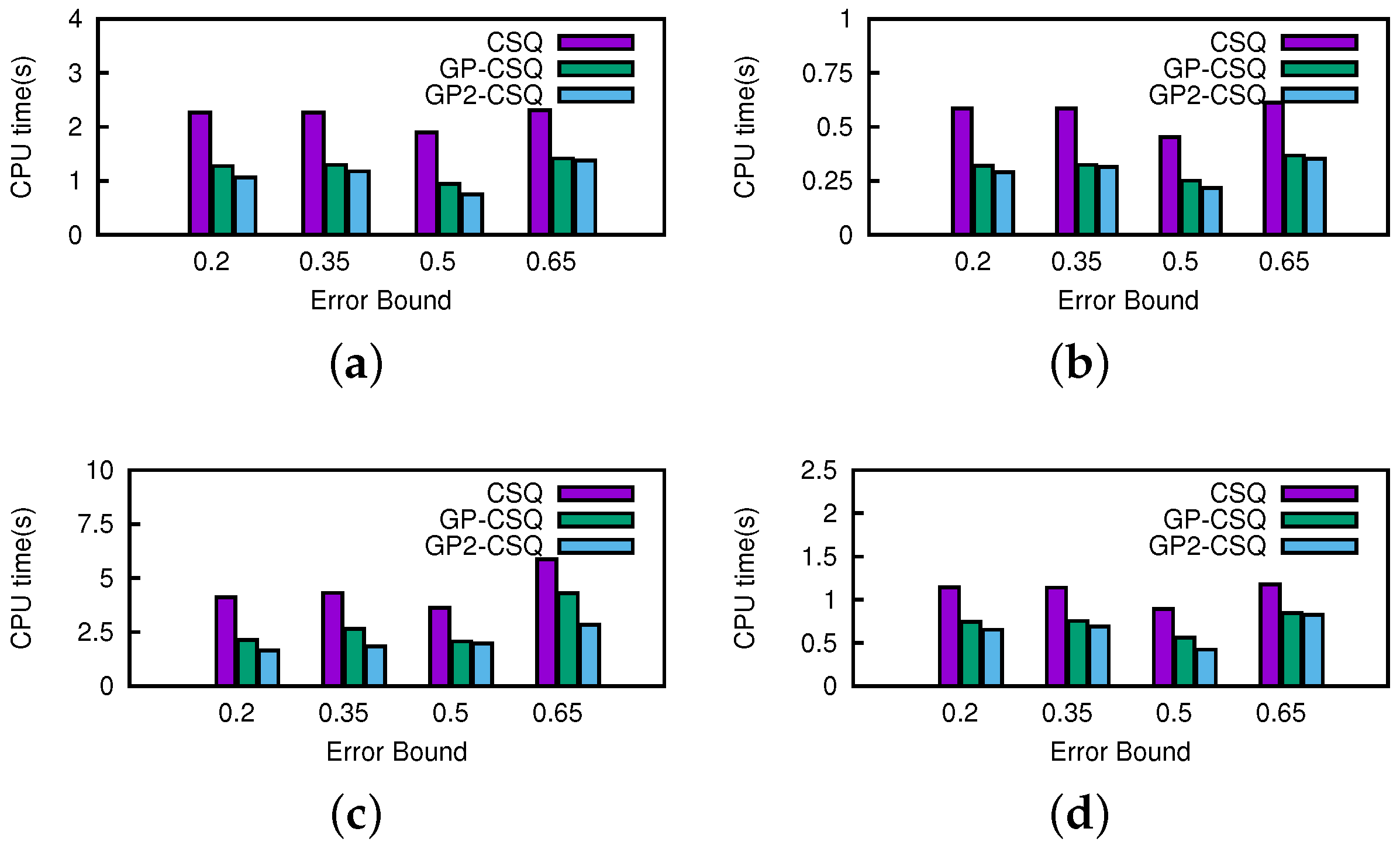
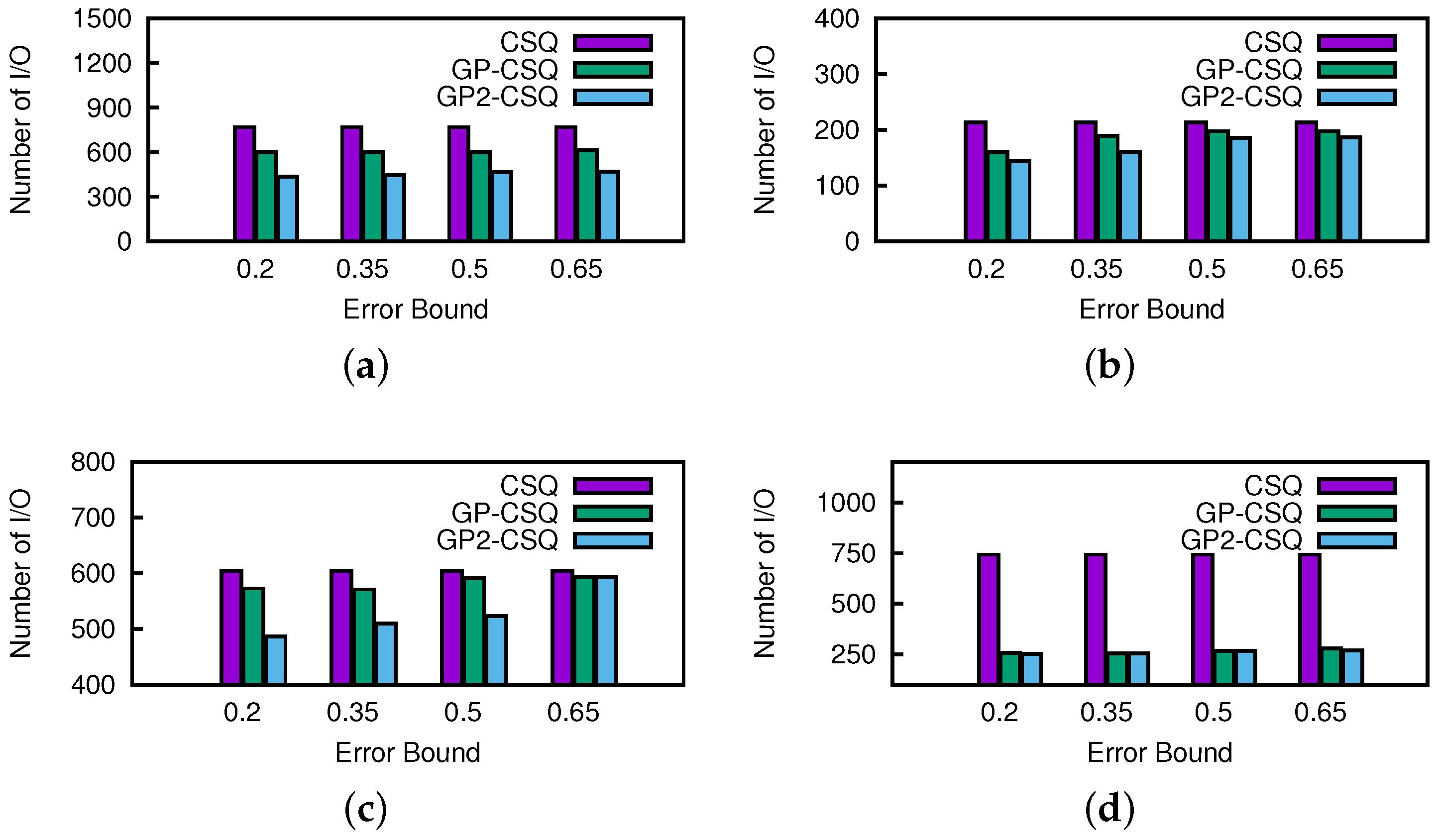
Effect of Error Bound. In this section, we change the setting of thresholds from 0.2 to 0.65 running on the California road network dataset. A higher threshold means that more data points can get in the skyline earlier or leave it later. In
Figure 21 and
Figure 22, as the thresholds get wider, the costs of CSQ increases slightly since more points remain in the skyline and create more events. Generally, the change of threshold would not cause a prominent effect on the costs of the GP-CSQ and GP2-CSQ methods. In particular, in
Figure 22c, the second-time pruning operations using Lemma 5 were evidently weakened by wider threshold, since the available region of data points to be pruned became too small and the distribution made it fail to filter out unqualified data points. The CPU cost was lower when the threshold was equal to 0.5 because the process of computing the probability of dominance checking is simplified to speed up the processing.
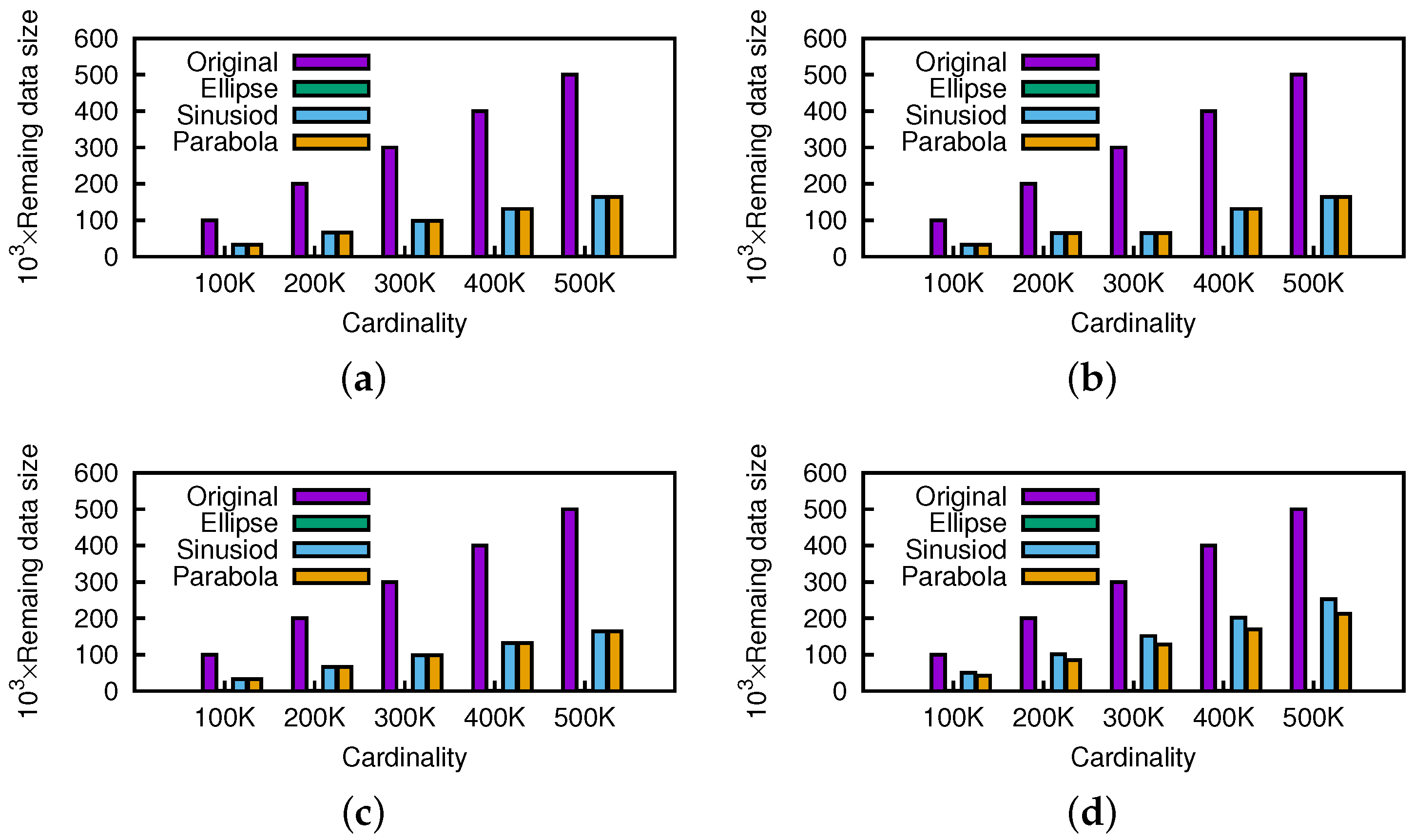
Geometric Pruning Framework Efficiency Evaluation. In this section, we compare the effect of the geometric pruning framework under different kinds of motion patterns (e.g., Enclosed, with Bounds, and without Bounds) to explore whether it is efficient and versatile enough. For simplicity, we take ellipse, sinusoid, and parabola as representative of the three motion patterns mentioned above.
Figure 23 shows that the geometric pruning framework works efficiently as the cardinality of each dataset increases. In particular, for the
ellipse, the pruning effect is very strong since we can eliminate most of the data points by invoking the geometric pruning algorithm several times for an enclosed motion pattern. More specifically, for the rest motion patterns, about 60% of the initial candidates were pruned out, which can still dramatically reduce the query execution time.
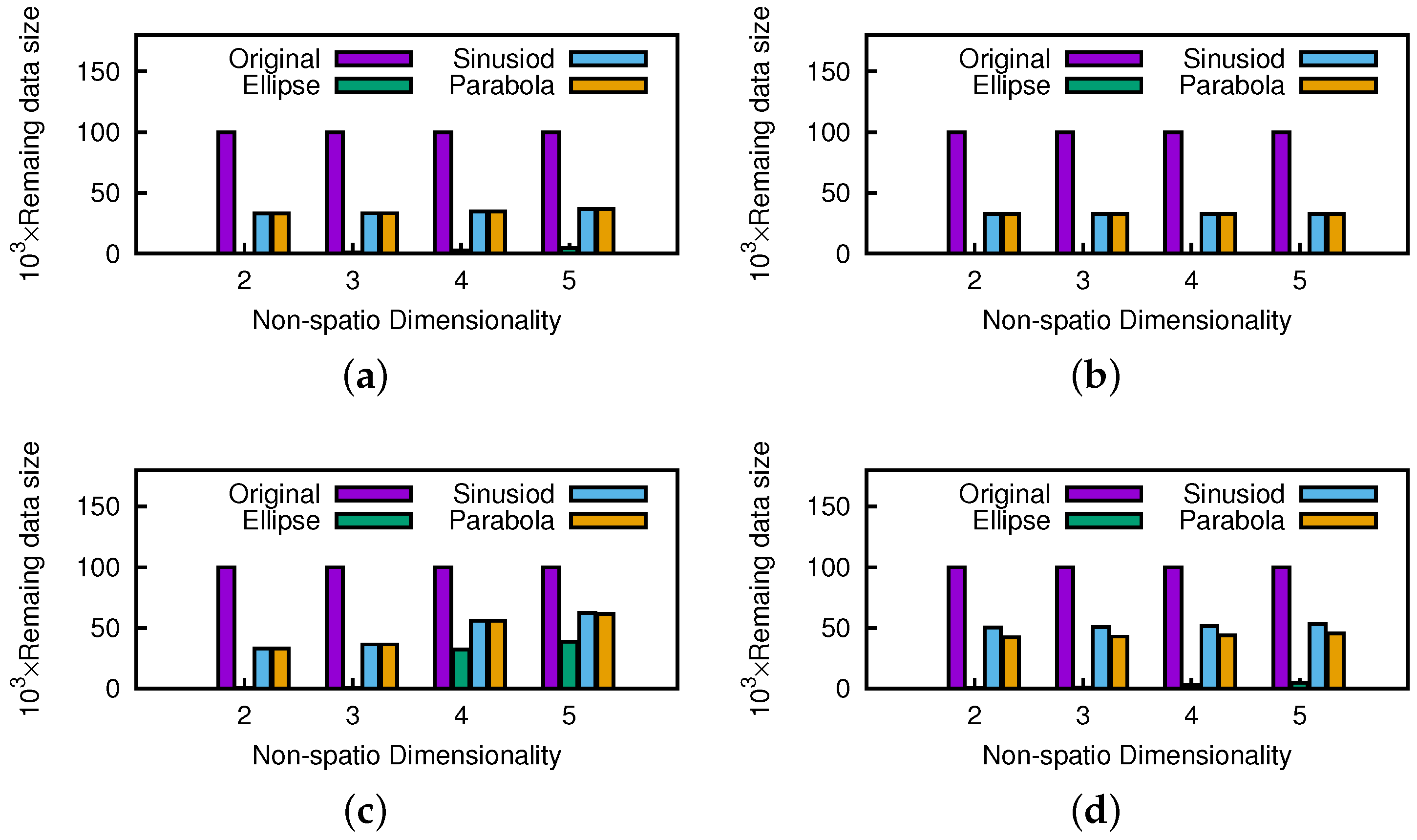
Figure 24 shows the influence of nonspatial dimensionality. The proposed pruning strategy is slightly affected by higher nonspatial dimensionality, since every data point will not be easily dominated in higher dimensionality, but the result indicates that it is still worth executing the pruning operations. Note that the remaining data sizes of the anti-correlated datasets are large due to their greater skyline results.
8. Conclusions
In this paper, we address continuous skyline queries on moving query points under the incremental motion model. Geometric properties are fully exploited to prune the data points which will not belong to the final skyline results, thus improving the efficiency of skyline query processing. Further, event-based mechanisms and a grid file index-based pruning policy are proposed to maintain continuous skyline results instead of computing skyline results from scratch. Two efficient algorithms (GP-CSQ and GP2-CSQ) are proposed based on geometric properties, and our extensive experiments have shown that the two geometric property-based algorithms are more effective and efficient than existing methods.
There are many promising future directions. Firstly, suitable motion patterns for specific applications can be found, and we can study how to alter the pruning strategies based on corresponding geometric properties to adapt the new motion pattern under our framework. Secondly, since we assume only query points and point attributes are dynamic, if the databases change (i.e., the data points are varying—insert, update, or delete), we can study how to develop efficient algorithms to answer user continuous skyline queries. Thirdly, future work can be devoted to investigating the possibility of using the proposed geometric pruning strategies to support other variants of skyline queries, such as reserve skyline queries [
24], skyline cubes [
29], spatial skyline queries [
16], probabilistic skylines [
27], and so on. While results obtained from comprehensive experiments indicated the superiority of our approaches devised based on the geometric pruning strategies over existing works, we believe that these explored geometric features and the proposed framework are useful for other skyline query variants not examined in this paper. Another interesting problem is to extend the geometric pruning strategies to other real applications (e.g., recommendation systems [
30], mobile sensor networks [
31,
32], and surveillance systems [
33]) such that whenever a query point is located, after a snapshot query is performed, by using the proposed geometric pruning strategies or other extentions, we can get the small part of candidates which may impact the query result in the near future without verifying all data points in the system so that the query results can be maintained efficiently according to the small-scale candidate datasets.


