3. A Point Location Query with Respect to a Line
In this section, we present an algorithm that, given a finite set of N points in , constructs a data structure of size . The data structure can be used to answer the following query in time: given as input a line ℓ in , return the points of P that are below ℓ, the points of P that are on ℓ, and the points of P that are above ℓ.
The latter algorithm receives a line ℓ as input in the form of a triple of real numbers that determining ℓ by the equation . In practice, these real numbers a, b and c have to be finitely representable. We can think of them as being computable reals or rational numbers, for instance.
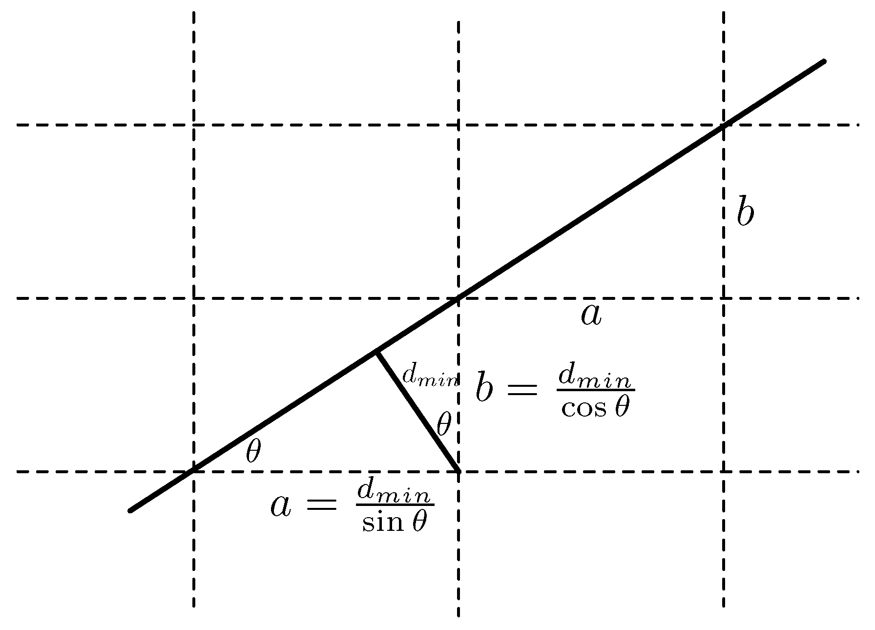
We would like to be able to order the values , for , such that it is easy to see which are less than, equal to or larger than 0. Indeed, those points of P for which are above the line ℓ, those points of P for which are on the line ℓ and those points of P for which are below the line ℓ. Therefore, ordering the values , and determining the indices where the sign changes from − to 0 and then to + would allow for answering the above query in constant time (apart from writing the answer, which necessarily takes linear time). It is easy to see that the ordering of the values is independent of c.
Obviously, there are
possible orderings of the elements of
P, or, equivalently, of their indices. Indeed, any ordering
of the elements of the set
can be seen as a permutation of this set. We write the permutation where 1 is mapped to
; 2 is mapped to
, ...., and
N is mapped to
as
We denote the group of all permutations of the set
by
. For
, we can consider the subset
of tuples
for which
The above inequalities can be equivalently written, independent of
c, as
The sets , determined this way, are linear, semi-algebraic subsets of the two-dimensional -plane. We have already remarked that there are at most such possible sets, since there are elements in . However, as we will soon see, the number of distinct sets is bounded by . Indeed, consists of (at most) linear inequalities in a and b. These inequalities can be written as , . Some of these may coincide, namely when, in the original set P, there are pairs of points that form parallel line segments. Geometrically seen, these inequalities divide the -plane in (at most) partition classes determined by the lines , for . These lines all go through the origin of the -plane, and determine at most (unbounded) half-lines. These half-lines divide the plane further in (unbounded) pie-shaped slices.
We remark that it is meaningless to consider the origin of the -plane, since no line corresponds to this point.
We illustrate this by means of two examples of increasing complexity.
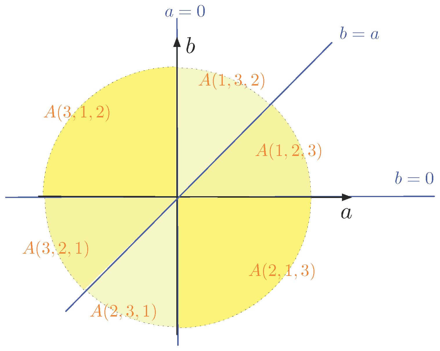
Example 2. First, we take and the points of P are , and . The following table gives the six possible orderings of the index set and the corresponding equations that describe the sets , for . | |
| |
| |
| |
| |
| |
| |
The sets are delimited by the lines , and in the -plane. This is illustrated in Figure 2. We remark that the sets are topologically closed and some of the sets share a border, which is a half-line (as can be seen in in Figure 2). For example, and share the positive a-axis as a border. For all points with , we have the orderings and , which coincide. Indeed, and both correspond to for . In the previous example, we have six sets . Exceptionally, for , we have . This is no longer true for larger values of N, as the next example illustrates.
In Example 2, we see that the set corresponding to the order and its reversed order , namely, and , are reflections of each other along the origin of the -plane. This holds for all in Example 2 (as indicated by the corresponding shades of yellow) and in general, as the following property explains:
Proposition 1. If , then .
Proof. Let . If , then and thus , which implies that . This proves one inclusion. The other inclusion has the same proof. ☐
The next, more complex, example adds one point to the set P of Example 2.
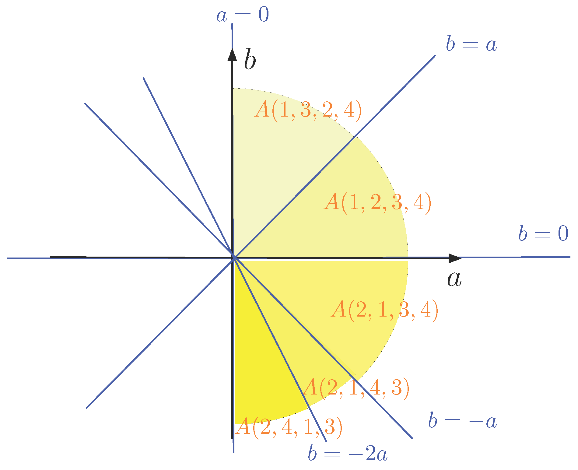
Example 3. Now, we take and the points of P are , , and . Property 1 shows that we only have to consider 12 of the permutations of the set . The following table gives these 12 orderings of the index set and the corresponding equations that describe the sets . | |
| |
| |
| |
| |
| |
| |
| |
| |
| |
| |
| |
| |
Because the line through and and the line through and , there are less than lines in the -plane that delimit the sets . In fact, they are five: , , , and (as also can be seen in the table). Thus, here the -plane is divided in ten half lines and ten pie-shaped slices, as illustrated in Figure 3. Half of the slices are not shown, but can be obtained via Property 1. Also not shown in Figure 3 are the facts that is the non-negative b-axis and that which does not correspond to any line. Therefore, we have . These observations show that typically not all (or ) sets will occur separately. Now, we illustrate the construction of the data structure
for Examples 2 and 3. The structure
essentially is an AVL tree. AVL trees, named after Adelson-Velsky and Landis [
11], are binary search trees. This means that, at each of its nodes, the items with key-values less than the node are stored in its left child subtree and the values larger than the key-value than the node are stored in its right child subtree. Binary search trees that store
m key-values, ideally, allow for searching for a given key value in time
. This time complexity occurs when the binary trees are fairly balanced. Whereas many node insertion and deletion methods may result in unbalanced binary search trees (with a search complexity that may become
, rather than
), the AVL tree method dynamically rebalances the AVL tree after insertions or deletions of nodes by applying a sequence of rotations or double rotations [
11]. The number of rotations and double rotations needed to rebalance the tree is linear in the height of the tree. AVL trees remain “balanced” in the sense that, for every node, the heights of the left subtree and the right subtree differ by at most one. The height of a tree can be defined as the length of the longest path from its root to a leaf.
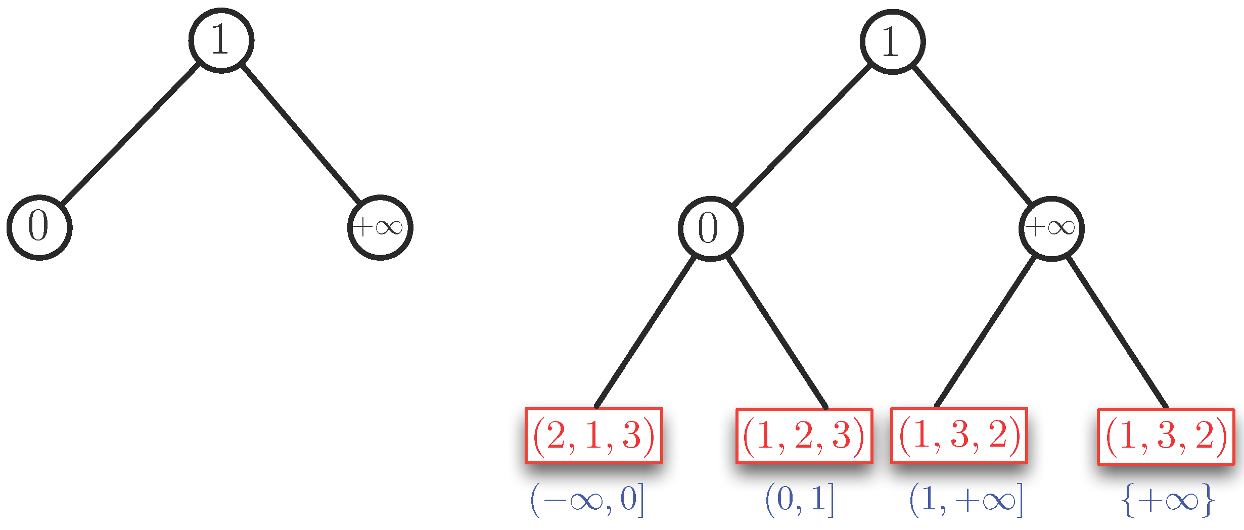
Example 4. We consider two cases: and . By Property 1, the case can be reduced to the case (using reversed orderings). Therefore, essentially, the case , remains to be solved. We assume . First, we order the slopes of the half-lines we find in the half-plane in the range . Here, we agree that the positive b-axis with equation is expressed as . In Example 2, we have the slopes , and , which give the ordering . We use these slopes as key values to build an AVL tree. For Example 2, this tree is shown in the left part of Figure 4. The corresponding data structure is shown in the right part of Figure 4. For this example, the AVL tree is perfectly balanced. The blue intervals under the leaves of the AVL tree show which parts of the interval correspond to a leaf. In this example, we have the following sequence of open-closed intervals at the leaves: , , and . There is a tiny redundance for the case , which is covered by two leaves. This only occurs when is a slope. The red boxes at the leaves show the ordering of (the indices of) the points in , for the interval of slopes at each leaf. Each red box represents (or contains) a binary search tree on the ordering (or permutation) that it contains.
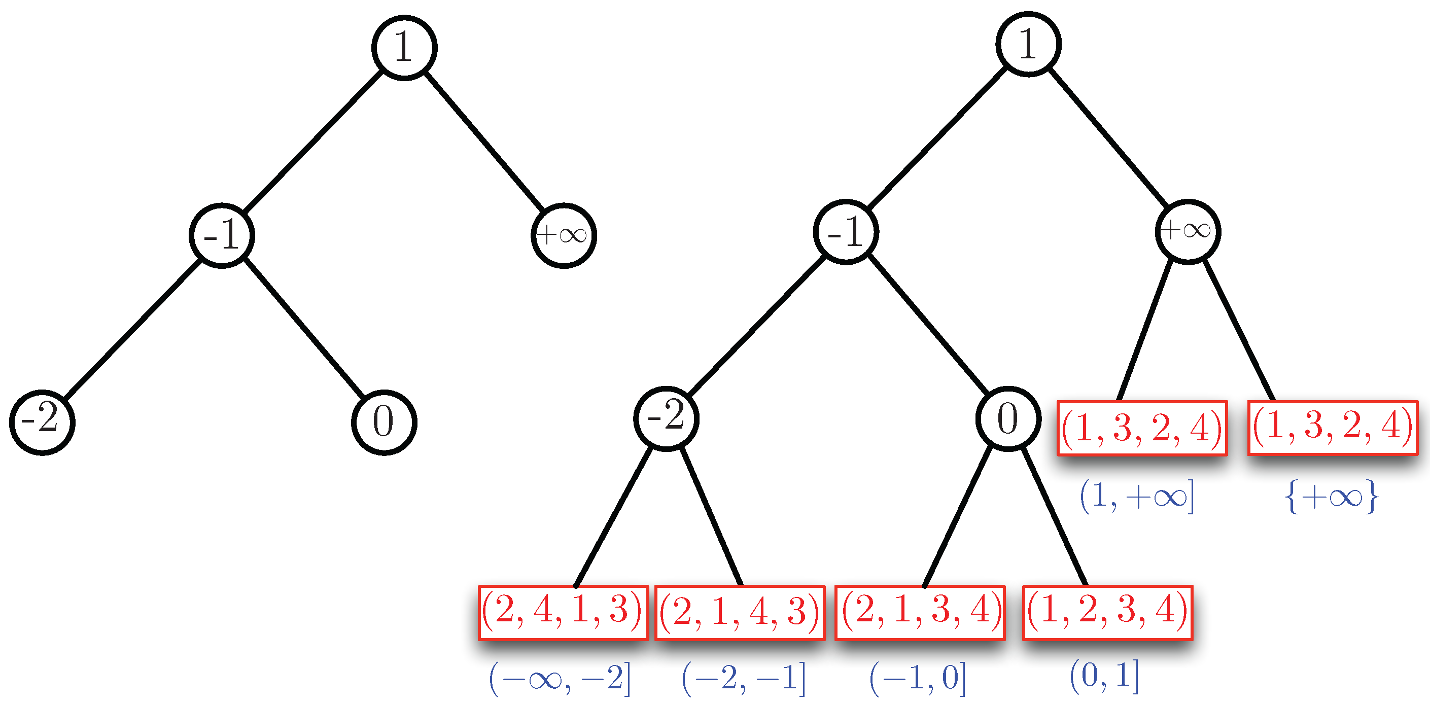
In Example 3, we have two additional slopes, namely and . This gives the ordering of the slopes. If we insert and in the AVL tree of Figure 4, we obtain the AVL tree and the structure for Example 3, as shown in Figure 5. In this example, the AVL tree is almost balanced. The height of the left subtree of the root is one higher than that of the right subtree. We remark that the height of the AVL is logarithmic in the number of its nodes. Since there are at most slopes, we have a height of . Therefore, we need time to find the leaf corresponding to the slope of a given line.
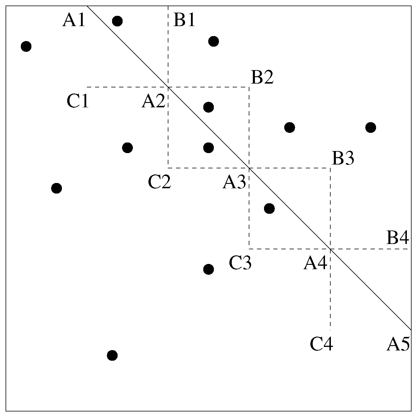
Now, we describe the lower lower part of the structure , which is represented by the red boxes in Figure 4 and Figure 5. To determine the permutation of the left-most, we pick an and b such that is strictly smaller than the first slope, which is . For instance, we can take and and remark that any other choice such that will give the same permutation. Then, we have to order , for , for and . This gives the ordering (or permutation) . For the next leaf to the right of this leftmost leaf, we do not need to redo the complete ordering process. Only points and for which can switch order when passing the slope . In this example, we see that the slope is caused by and and, indeed, 1 and 4 switch places in the permutation giving for the next leaf. We remark that the permutation information in the “red boxes” can be stored in a binary AVL tree itself. The search tree of Figure 5 can now be used to answer the half-plane range query. For instance, if the line ℓ with equation is given, we find the permutation at the leaf that corresponds to the interval in which the slope is located. To see which of , , , are below ℓ, we compute for (in that order) as long as this value remains strictly below . In this case, only is found to be below ℓ. We now show the following theorem that generalizes Examples 2, 3 and 4. The proof will follow the ideas outlined in the examples.
Theorem 2. Given a set of N points in , a data structure of size can be constructed in time such that for any input line ℓ in , given by an equation , it is possible to determine from in time which of the N points are below, above, and on the line ℓ.
The data structure can be updated in time when a point is added to P or deleted from P.
Before we prove this theorem, we remark that the complexity of determining from , which, of the N points, are below, above, and on the line ℓ takes time. This does not include writing the answer when this is required. Obviously, writing this ordering necessarily may take linear time. However, effectively listing these points may not be necessary if the answer is allowed to be a pointer in a search tree and the actual answer consists of “all the points that precede this point”. This is possible because the permutation of points itself can be put into a binary (AVL) tree. Now, we give the proof of the theorem.
Proof. Given a set of N points in , we first determine the slopes in the -plane of the lines , for . There are at most such slopes, as some may coincide. This takes time and space.
Now, as we have illustrated in Example 4, we concentrate on the half-plane, determined by
. To deal with the case
, we can use Property 1. At this point, we can build the upper part of
by constructing an AVL tree on the slopes (in the way we have illustrated in Example 4). Since the cost of inserting a node in an AVL tree with
n nodes is
, the cost of building an AVL tree of
n nodes, by inserting these
n nodes one after the other, is
and the tree takes
space. Applied to our setting, we have at most
slopes, so building the AVL tree on these slopes takes
time and
space. Building the AVL tree produces, as a side effect, an ordering of the slopes, if we look at the leaves of the tree from left to right. This way, we also obtain the interval information, given by the blue intervals in
Figure 4 and
Figure 5.
After the AVL tree is built, we need to determine the order of (the indices of) the points of
P at each of the leaves of the tree. These orders are illustrated by the permutations in the “red boxes” in
Figure 4 and
Figure 5. Let the slopes that occur in the AVL tree be
, with
By taking some arbitrary
and
b such that
and ordering
, for
, we obtain the permutation that is in the leftmost leaf of the AVL tree. We can store this permutation (in the red box) as an AVL tree itself. It takes
time and
space to build this smaller AVL tree to store the ordering. For the next leaves (going from left to right in the tree), as we cross some slope
, only the order of indices
i and
j switch, compared to the previous leaf, if
Indeed if, for instance for , then we have for . This implies that, going from left to right through the leaves in the AVL tree, we can update the permutations in linear time in N.
Since the AVL tree has leaves, the total time to construct the structure is . We have the same space bound. We remark that the total height of the structure that we obtain is .
The query time complexity is the following. On input line ℓ, given by the equation , it takes time to determine the leaf of the AVL tree that contains the interval in which the slope is located. Indeed, the height of the AVL tree is logarithmic in the number of its nodes, which is . Let us assume that this leaf contains the permutation (in its red box). To output the points that are below ℓ, we write to the output for as long as . In the worse case, the output contains all points of P. Obviously, this writing process takes linear time in the size of the output.
Finally, we discuss updating the AVL tree when a point is added to P or a point is deleted from P. Adding or deleting a point can cause the introduction or removal of at most N slopes. Adding or deleting N slopes in an AVL tree takes time. Finally, the permutations in the leaves need to be updated. We remark that, since the permutation lists are themselves stored as AVL trees, then deleting a point from P results in deleting one leaf from the AVL tree in the red boxes. Similarly, adding a point to P results in adding one leaf to the small AVL trees. This has an update cost of . The total update time is therefore This concludes the proof. ☐


