1. Introduction
Triangulated irregular networks (TINs) provide one of the basic ways to represent surfaces in GIS. A TIN is constructed from a set of sample points, by triangulating the points in 2D. The resulting triangulation gives a continuous interpolating surface that is piecewise linear, in which each face is a triangle. The elevations of the vertices of the triangles are known, since they correspond to sample points, while the elevation for any other point can be computed by linear (or higher degree) interpolation based on the triangle containing it. It is well-known that a set of two dimensional points can be triangulated in many different ways. For surface modeling, the choice of the triangulation can make a big difference: different triangulations can result in entirely different interpolating surfaces. However, in practice, the question of what triangulation to use rarely arises while constructing TINs with GIS: most GIS will simply use the Delaunay triangulation.
The Delaunay triangulation (DT) is defined using the so-called Delaunay criterion: a triangle is Delaunay if the circle defined by its three vertices does not contain any sample point. A triangulation is Delaunay if all its triangles are Delaunay. In general, unless there are four or more points lying on exactly the same circle, the DT is uniquely defined by the point set. There are many good reasons for the DT to be the standard choice for TINs. The main one is that the DT is considered to have well-shaped triangles: triangles that are close to equilateral. This is because, among all possible triangulations of the same set of points, the DT maximizes the minimum angle of all triangles, avoiding slivers (long and skinny triangles) as much as possible. Slivers are a major concern in triangulations for terrain modeling, since they usually result in high interpolation error, can create visual artifacts, and operations with them are prone to roundoff errors, among other problems. Another important advantage of the DT is that it can be computed efficiently, and with relatively simple algorithms.
However, the DT in 2D suffers from one major limitation: it only considers the 2D coordinates of the sample points, i.e., it ignores all elevation data. This means, for instance, that two sets of sample points with the same 2D distribution will end up with exactly the same triangulation, no matter how different the original surfaces were. This can result in an interpolating surface that does not adapt to the real topography, producing a poor approximation.
Realizing that an accurate surface approximation should take into account all data available, Dyn et al. [
1] introduced the concept of
data-dependent triangulations, defined as triangulations that are optimal with respect to criteria that involve all three coordinates of the data. For example, for surfaces that are rather smooth, Dyn et al. [
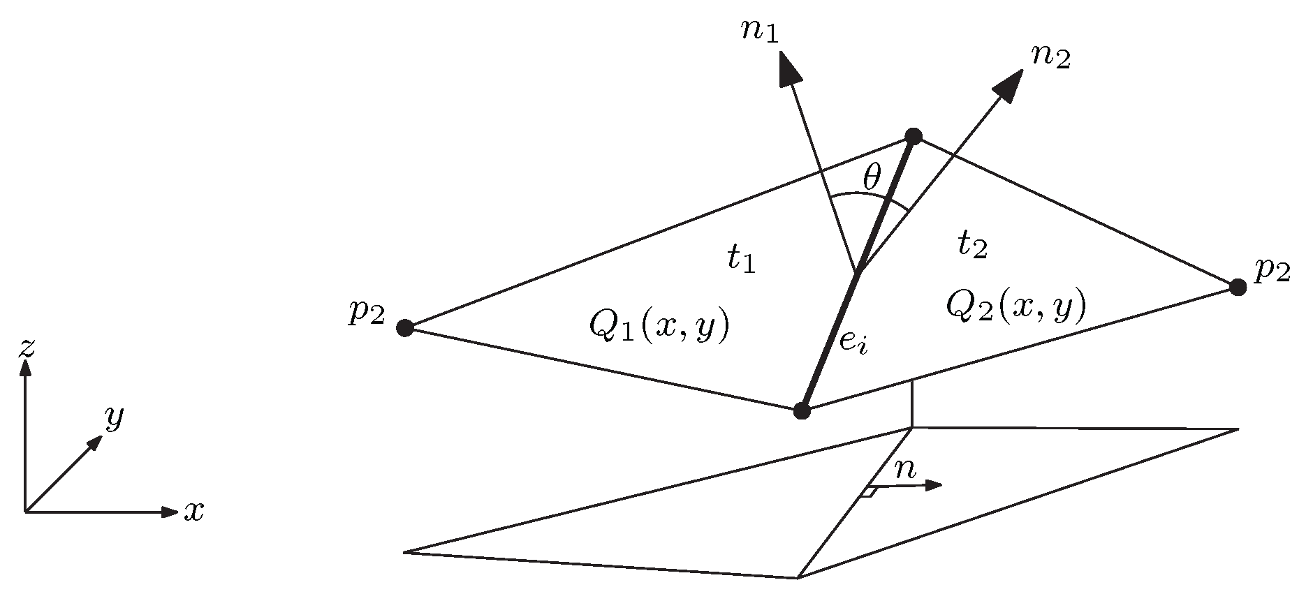
1] concluded that the criterion of minimizing the angle between the normal vectors of adjacent triangles gives better results than the DT. Later studies [
1,
2,
3,
4,
5] about data-dependent triangulations arrived at similar conclusions, and proposed other data-dependent criteria to improve over the DT. Despite this, in most GIS software today, the DT is still the only choice to triangulate points. The main reason for this is that, even though data-dependent criteria can improve some aspects of the approximation, they often produce too many slivers [
4,
6]. Thus, the advantages obtained by data-dependent criteria are outweighed by the negative effects of ill-shaped triangles. It follows that an ideal triangulation method should be able to combine both approaches: aim at optimizing relevant data-dependent criteria, while at the same time trying to avoid slivers [
4,
6].
The problem of combining good triangle shape with data-dependent criteria was also studied in the field of computational geometry. Gudmundsson et al. [
7] proposed
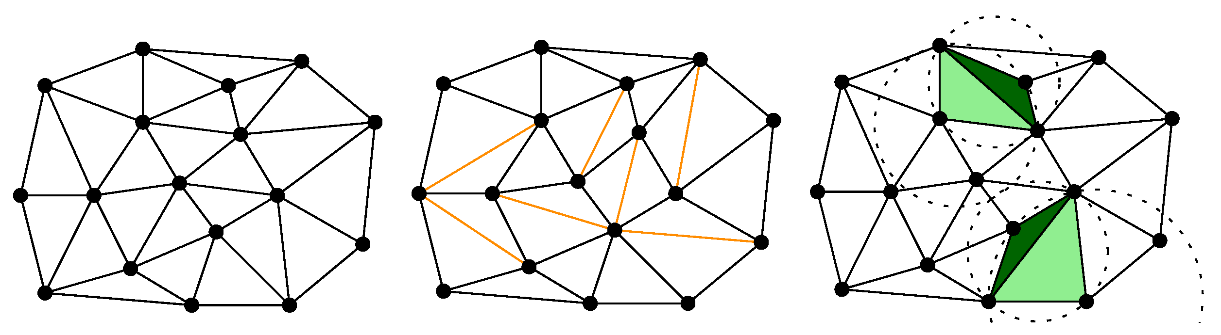
higher order Delaunay triangulations (HODTs): a generalization of the Delaunay triangulation that offers well-shaped triangles, but, at the same time, flexibility to optimize extra criteria. HODTs are defined by allowing up to
k points inside the circles defined by the triangles, for
k a parameter called the
order of the triangulation (see
Figure 1). Formally, a triangle
in a point set
S is
order-k Delaunay if the circle defined by
u,
v and
w contains at most
k points of
S. A triangulation of
S is
order-k Delaunay if every triangle of the triangulation is order-
k.
For , any set of points (in which no four points are cocircular) has only one higher order Delaunay triangulation, equal to the DT. As k is increased, more points inside the circles imply a potential reduction of the triangle shape quality, but also an increase in the number of triangulations that are considered. This last aspect is what makes the optimization of extra criteria possible: for each order , there is potentially a whole family of different triangulations with well-shaped triangles, among which one can choose the one that is best according to some other, data-dependent, criterion.
Some theoretical studies about HODTs have studied the number of HODTs that one can expect, as a function of the number of points
n and the order
k. However, most of that work has focused mainly on determining, which criteria can be optimized efficiently (i.e., in polynomial time) and which of them are intractable (i.e., NP-hard), either for general values of
k, or for the simpler case of
. Positive results in this direction can have important practical implications if they come with easy-to-implement methods to optimize the criteria. As already mentioned, for points drawn uniformly at random, the expected number of different triangulations is exponential already for
, roughly larger than
[
8]. This is encouraging from a practical point of view because it implies that there should be many triangulations to choose from to optimize data-dependent criteria. However, having a large number of triangulations available does not guarantee that some of them will be significantly better than the DT with respect to data-dependent criteria. Also of theoretical interest, there has been some preliminary studies about how to enumerate all order-
k triangulations, although results so far are limited to very small orders
[
9].
The more practical aspects of HODTs have not been studied much. The few papers that have studied and implemented optimization algorithms for some concrete criteria for real terrains [
10,
11,
12] have focused on very specific criteria. Namely, the minimization of pits, avoiding interrupted valley lines, and slope fidelity. In all cases, heuristics were presented, and a few experiments with real terrains were shown. However, one important conclusion that can be drawn from these studies is that even though the exact optimization of these criteria is algorithmically difficult, local optimization heuristics can give important improvements for very low orders of
k. For instance, experiments for orders
with real terrain data by [
12] found that, for minimizing the total number of pits, the reductions obtained can be of 15–20% for
, and of up to 50% for
.
Being a generalization of the DT, in terms of optimizing a data-dependent criterion, the use of HODTs will always give better, or at least not worse, triangulations than the DT—always from a data-dependent point of view. This can be explained by the fact that, by definition, the set of order-k Delaunay triangulations includes all those of order less than k (thus including the Delaunay triangulation, which is a 0-OD triangulation). To this point, it is important to note that this does not imply that there will be always a k-OD triangulation with order greater than zero that is better than the DT but, since there are more options, there may be the possibility of this happening. Therefore, the key question with HODTs could be stated as whether HODTs are worth the effort. Firstly, optimization software for HODTs is not readily available, thus using HODTs instead of the DT implies, at least, a certain implementation overhead. Secondly, optimizing over all HODTs of a certain order, even , will necessarily imply a longer running time than simply computing the DT.
Hence, several important practical questions arise: (i) How much improvement does it give over the Delaunay triangulation? (ii) Do higher order Delaunay triangulations actually preserve the good shape of the triangles, as expected in theory? (iii) How complicated is it to implement some type of optimization over HODTs? In this paper, we try to answer these questions.
There is very little previous work devoted to the more practical aspects of HODTs. Only a few papers have studied the optimization of concrete data-dependent criteria for real terrains [
10,
11,
12]. They focused on very specific criteria related to the minimization of pits, avoiding broken valley lines, and slope fidelity. Ad hoc heuristics were presented for each of them, and a few experiments with real terrains are shown. The results suggest that simple heuristics for optimizing those criteria for low orders (
1.8) can give a significant improvement over the Delaunay triangulation.
Contributions. We present an extensive study on the practical use of HODTs, as a way to build data-dependent triangulations. Our main goal is to evaluate whether the improvements in the data-dependent criteria that can be obtained by using HODTs, compared to the Delaunay triangulation, are significant enough as to justify implementing a more complex triangulation algorithm. Our secondary goal is to describe some of the implementation aspects of HODTs, never considered until now.
We selected three data-dependent criteria that have been claimed in the literature to give the most important improvements over the DT (
angle between normals,
jump normals derivatives,
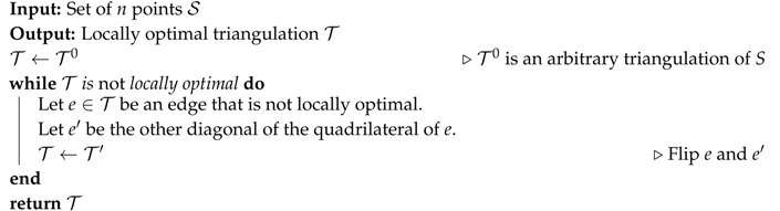
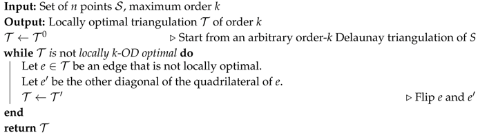
refined angle between normals). We implemented and tested two variants of an optimization algorithm based on the well-known
Lawson’s Optimization method (LOP) [
13]. This method was chosen due its simplicity and generality: it is easy to implement, and can be used to optimize any criterion. In addition, we also implemented and tested the exact algorithm by Van Kreveld et al. [
14] for first order Delaunay triangulations. In fact, we implemented two variants of this method as well: the algorithm as proposed in [
14], and a simple variant that improves the shape of the resulting triangulation even further, by prioritizing Delaunay triangles. This is the first time that the algorithm by Van Kreveld et al. [
14] is implemented and evaluated experimentally.
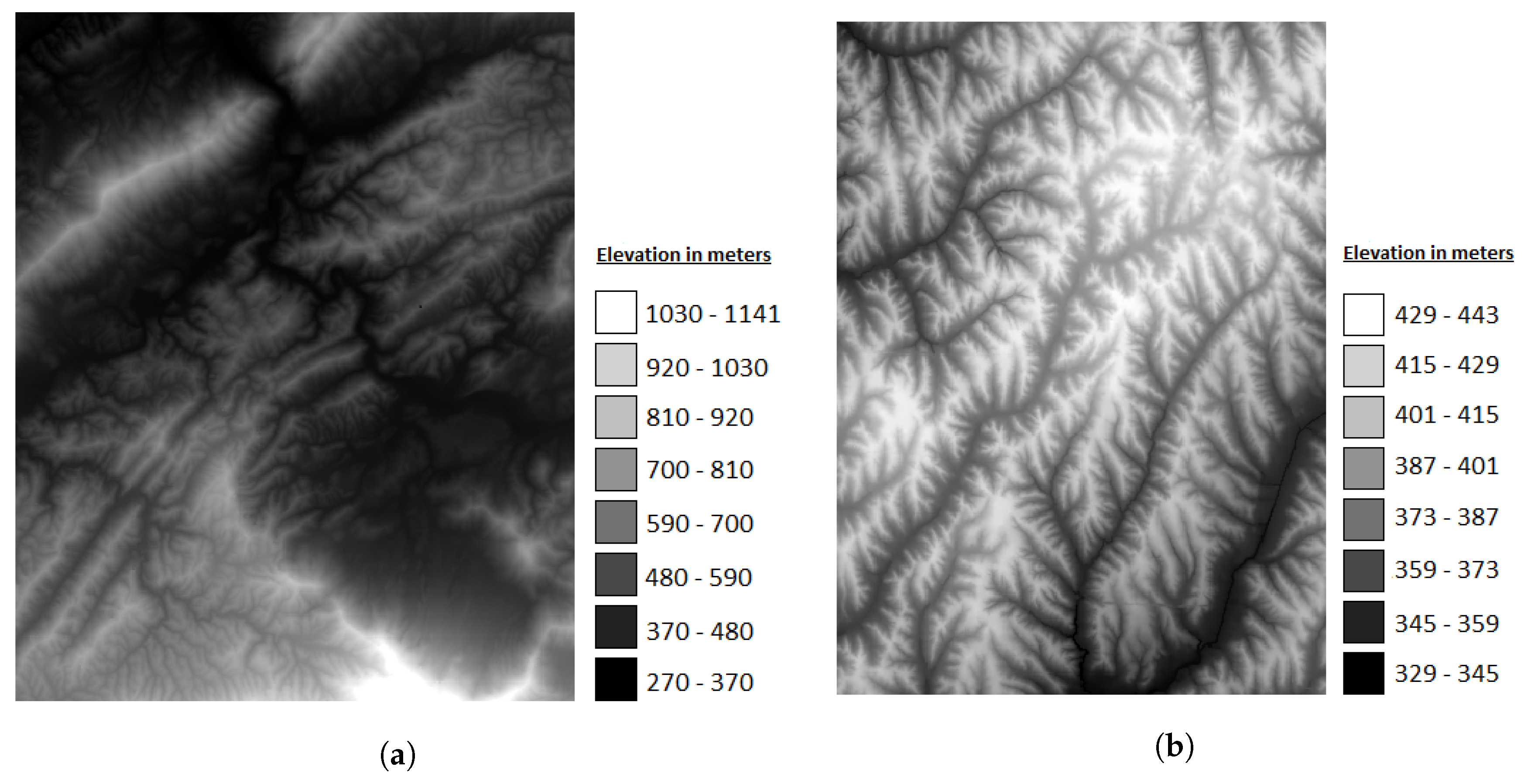
We present experiments with real terrains for each criterion, measuring the improvements obtained by optimizing over HODTs. Data used was obtained from the two USGS terrains used in [
4], the most extensive previous study on data-dependent triangulations on real terrains. Our experiments cover different values of Delaunay order
k, different optimization algorithms, and evaluate the value obtained for each criterion, together with several other parameters of interest. The decision to use natural terrains, as opposed to synthetic terrains, as done in early related work [
1,
3,
15], is motivated by the fact that it has been questioned whether synthetic terrains are suitable to evaluate data-dependent triangulations [
4,
6]. Thus, it becomes particularly interesting to evaluate whether improvements observed for synthetic terrains for data-dependent triangulations also show up with real terrains using HODTs.
Our experiments shed some new light on the efficacy of three data-dependent criteria that, despite having been proposed a long time ago, had only been tested on real terrains a few times. Our results also show that a simple optimization heuristic for HODTs, similar to LOP, can give substantial improvements over the data-dependent criteria studied, already for very low orders (thus with triangles close to Delaunay). Therefore, we conclude that HODTs can be considered a practical tool to implement data-dependent triangulations, and that the benefits obtained are worth the extra overhead of implementing them, if improving on the data-dependent criterion is important.
4. Results
The amount of data generated makes it hard to present all results in tabular form. Nevertheless, as a sample, we present in
Table 1 the results obtained for ABN and the larger terrain sizes. It will be more convenient to analyze the results through the graphs presented in
Figure 4,
Figure 5,
Figure 6,
Figure 7,
Figure 8,
Figure 9 and
Figure 10. In the following, we discuss briefly the results obtained for the different aspects evaluated. In general, we do not observe a clear difference in behavior between the smaller and larger terrain sizes (i.e., 1% and 3%).
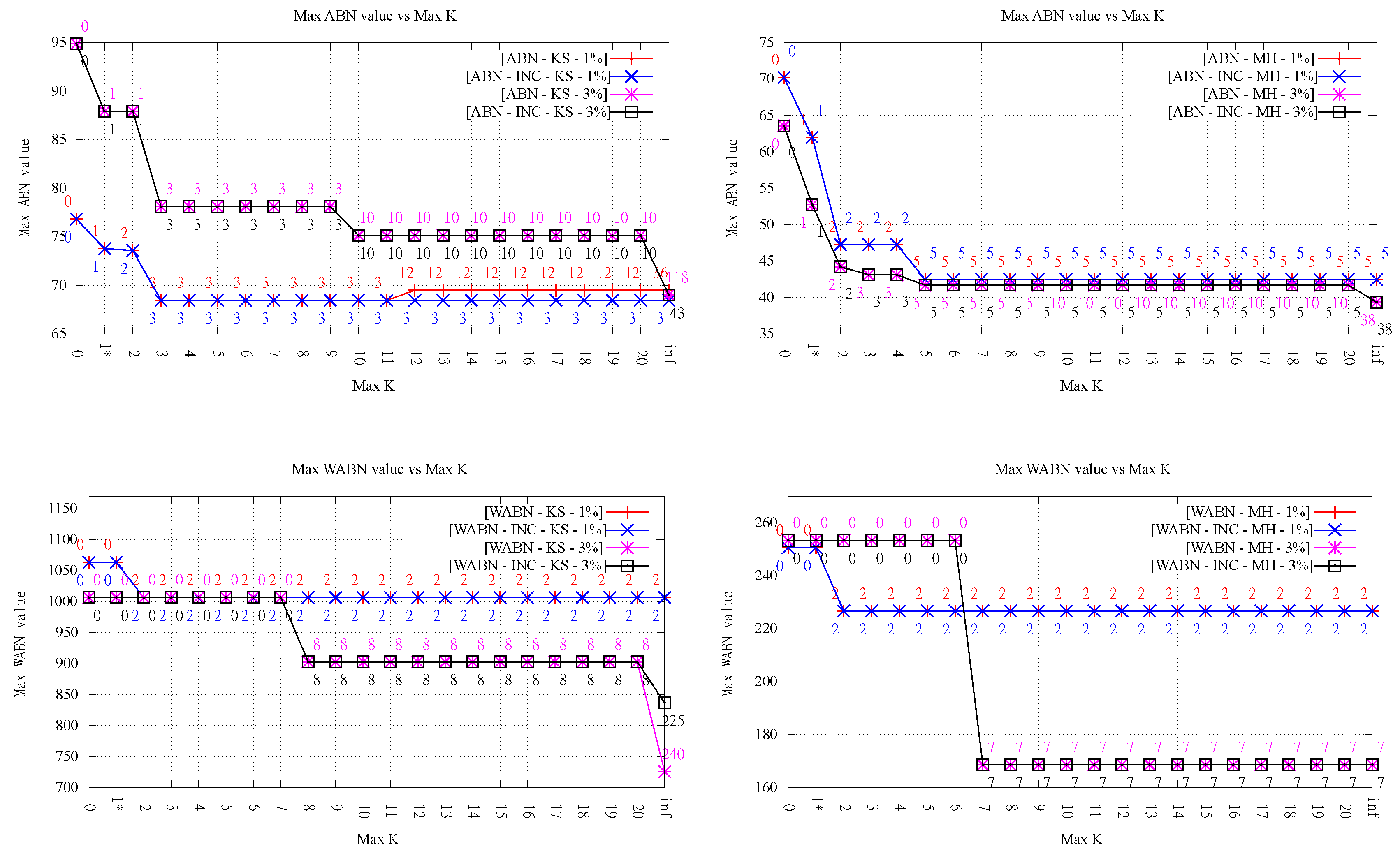
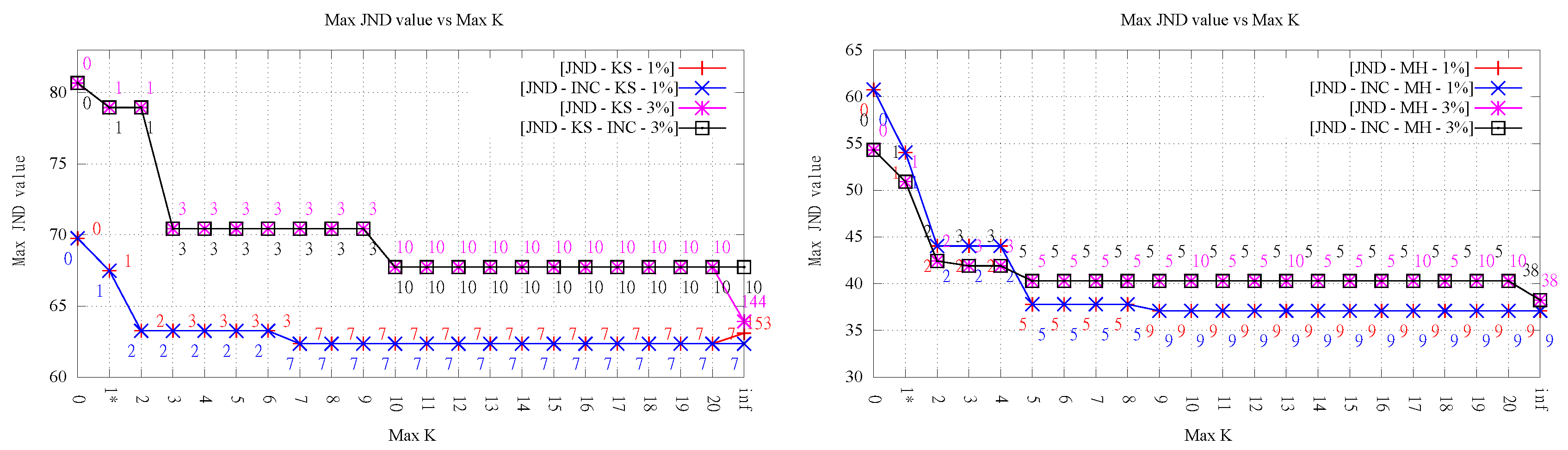
4.1. Maximum Value
Figure 4 presents the maximum value obtained for each measure, for the different orders
k, both terrain sizes, both LOP variants, and both exact implementations.
It can be observed that, in general, increasing the maximum order allows for improving all three measures significantly. For both LOP variants, the reductions obtained with respect to the Delaunay triangulation for orders were between 5.35% and 39.50%, with an average of 12.12% for Kinzel Springs and 30.27% for Moorehead SE.
Another important observation from
Figure 4 is that, in the majority of cases, significant improvements were obtained for very low orders. Even more, in many cases, the result obtained for low orders is as good as the one for infinite order, and, when this is not the case, often the difference was small.
For the LOP-0 implementation, it can be observed that, in most cases, increasing the maximum order
k results in a measure value as good or better than for the previous order. However, we observed in two settings (KS-ABN and KS-JND) that the max value became slightly worse after increasing
k. Since this may appear counterintuitive, it is worth explaining the phenomenon. This is basically due to the fact that executions of LOP-0 for consecutive values of
k are totally independent. That is, they always start from the Delaunay triangulation. This means that the flip decisions taken during the execution for order
k need not be a subset nor related to those taken for
, explaining that the end result can be worse than the previous one. In fact, for the same reason it can also occur that the final order of the resulting HODTs for order
k is lower than that for order
(always respecting the maximum order). This behavior is in contrast to that of LOP-INC where, by construction, the value decreases monotonically with
k. However, it must be noted that this fact does not necessarily imply that LOP-INC performs always better than LOP-0 in terms of minimization of the maximum value (see, for instance, the case of WABN for Kinzel Springs over 3% sample with
in
Figure 4). What may happen for LOP-INC with respect to LOP-0 is that a flip used to produce the starting triangulation for order
k prohibits a better flip in the construction of the
k-ODT, resulting in a maximum value higher than the one obtained by performing such restricted flip. Thus, the resulting
k-ODT will always have a measure value less or equal than the one in
-ODT but not necessarily better than the one measured in the
k-ODT obtained by LOP-0.
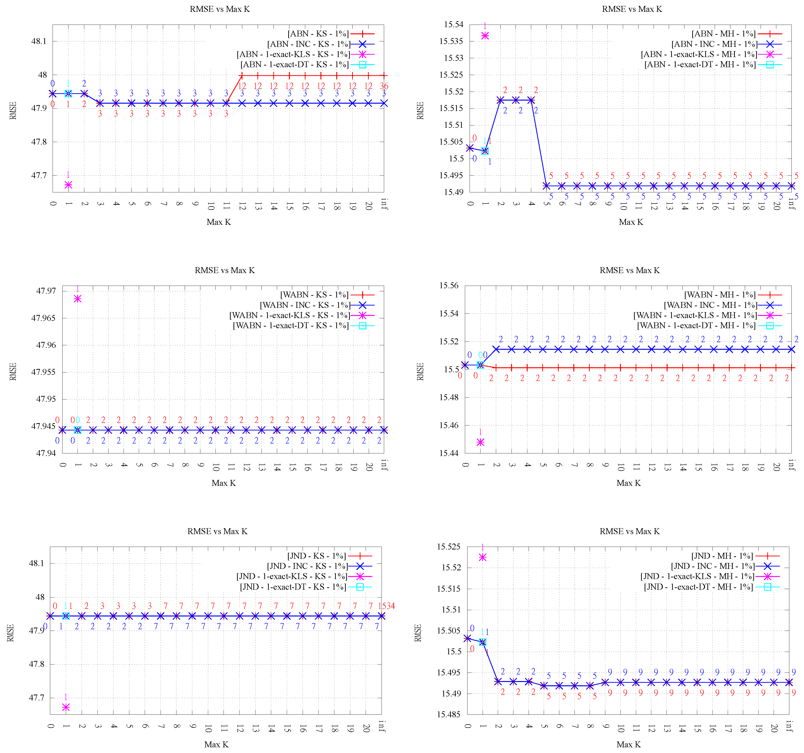
4.2. Quality of Approximation
Despite the clear improvement in the measure values shown in the previous section, the trend in the quality of approximation of the TINs, as measured by the RMSE based on the ground truth points, is less clear. This is rather relevant because this is arguably the most important metric motivating the use of data-dependent triangulations.
Analyzing the results for LOP-0 (a total of 12 evaluations, shown in
Figure 5 and
Figure 6), for low orders (
), and ignoring the particular case of
k = 1-exact (discussed in
Section 4.4), we can see that the RMSE stays roughly constant or decreases in nine cases (four and five, respectively), while it worsens in the other three cases. In all cases, the variation is rather small, something understandable given that the changes in the triangulations for
affect relatively few triangles, and thus have a limited impact on the overall RMSE. The fact that in some cases the RMSE gets worse is interesting, given that, in early work on data-dependent triangulations, it was argued that one of the reasons to optimize angle-related measures like ABN was to improve the approximation quality. It is also interesting to note that the results do not vary much for
; on the contrary, they are slightly worse (RMSE stays equal, decreases or increases in three, four, and five cases, respectively).
Overall, we can conclude that the approximation error in most cases does not get worse or even improves slightly, but not always, and that constraining the order of the triangulations has a positive effect, in comparison with the pure data-dependent approach (i.e., the case ).
The conclusions with respect to the overall behavior of RMSE for LOP-INC are the same as that for LOP-0. The differences in the final RMSE values observed between both algorithms are inherent to the fact that both methods are heuristic. It is important to note that even though the final order of the triangulation may be the same, this does not necessarily imply that the flips performed are the same (in other words, they do not produce necessarily the same triangulations). For that reason, there are cases where we observe different RMSE values for the same value of k. In some cases, the error is better for LOP-INC (for instance, in KS-ABN 3%), while, in some other runs, LOP-0 produced smaller error (for instance, in MH-ABN 1%).
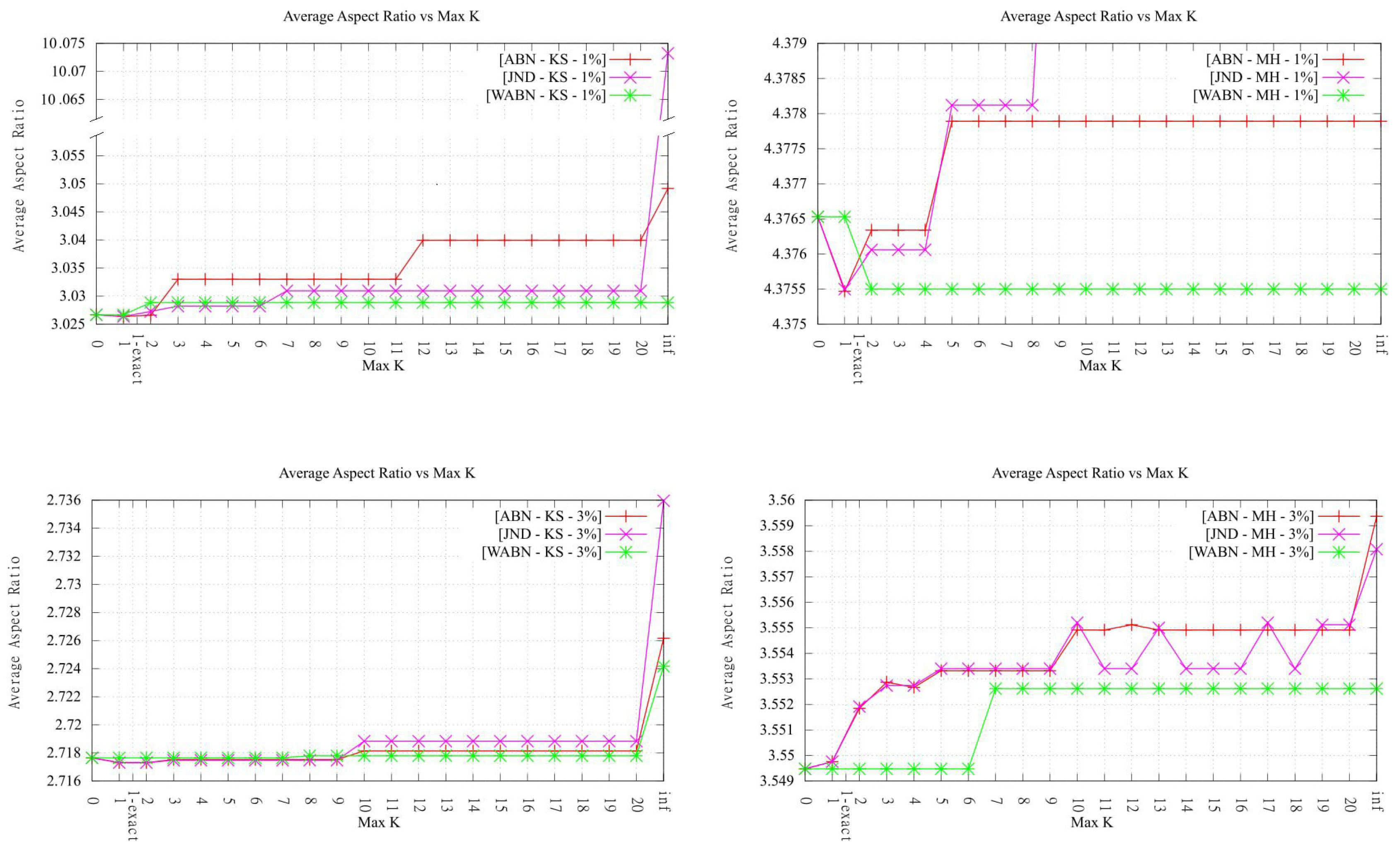
4.3. Presence of Slivers in HODTs
To evaluate if the increase in order resulted in an important increase in the presence of slivers, we measured the
average aspect ratio of the triangles in each final triangulation, as previously done in [
4]. From the results, it can be observed that, except for the exact algorithm from [
14] (1-exact-KLS) analyzed in
Section 4.4, the values remain more or less low (i.e., similar to the ones measured in the original Delaunay triangulation) and lower for lower
k order (maximum and final) values. This indicates that HODTs do not change significantly the shape of the triangles, with respect to the Delaunay triangulation. Most tests for
(except for one, Kinzel Springs JND) also resulted in only a mild increase in aspect ratios. This behavior, which is likely to be rather terrain-dependent, is probably explained in this case by the fact that the average aspect ratio is hard to change significantly by only a few flips.
4.4. Comparison between Heuristic and Exact Algorithm for k = 1
Regarding the performance of the exact algorithm for
from [
14], there are two aspects worth mentioning.
Firstly, the maximum values obtained by both variants of the exact algorithm for
were in all cases equal to the ones obtained by
k-OD LOP (see
Figure 4). In other words, for
, our modified LOP procedures obtained the optimal value in all cases. This is particularly interesting given that all but one case already presented improvements for
.
Secondly, it can be observed that, for the 1-exact-DT, the
average aspect ratio remains equals to the one measured in the heuristic. This is explained by the fact that by prioritizing Delaunay edges (only performing a flip when it actually improves the target value) only a few changes are done to the original DT in order to obtain the best 1-ODT. In
Table 2, it can be observed the differences between the amount of flips performed by 1-exact implementation from [
14] (1-exact-KLS) and the variant (1-exact-DT). Note that the number of flips performed by 1-exact-KLS lead to a higher
average aspect ratio than the one observed for 1-exact-DT.
Thus, the average aspect ratios were significantly worse for the exact algorithm from [
14] (1-exact-KLS), and something similar holds for the RMSE metric in several cases (see
Figure 5 and
Figure 6). As we mentioned before, this is due to the fact that the exact algorithm 1-exact-KLS makes no attempt to preserve the original Delaunay edges, since its only concern is minimizing the maximum value. On the contrary, in
k-OD LOP, the starting triangulation is Delaunay, thus most edges in the final triangulation are Delaunay as well. This results in better overall triangular shape, even though the worst triangles are the same. On the other hand, the variant 1-exact-DT, did not affect the maximum measure value and exhibited low average aspect ratios (see
Table 2). It is worth noting that, in every case, the 1-ODT obtained by 1-exact-DT is the same that the one obtained by the heuristic for
.
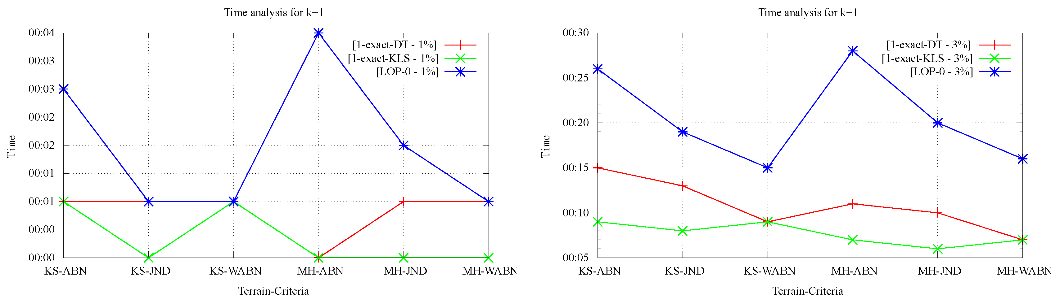
On the positive side, as shown in
Figure 7, the running times of the exact algorithms were in every case lower than that of 1-OD LOP being that difference more significant for the larger data sets. It’s worth noting that, by construction, running time measurements for LOP-INC and LOP-0 for
coincide thus, only the data for LOP-0 is presented in
Figure 7. Regarding the comparison of running times between both 1-exact variants, it can be observed that for 1-exact-DT time measurements are always worse or equal than those observed for 1-exact-KLS. This is explained by the overhead that exists in the 1-exact-DT implementation when verifying whether or not it is worth doing the flip suggested by the result of the 2-SAT solver.
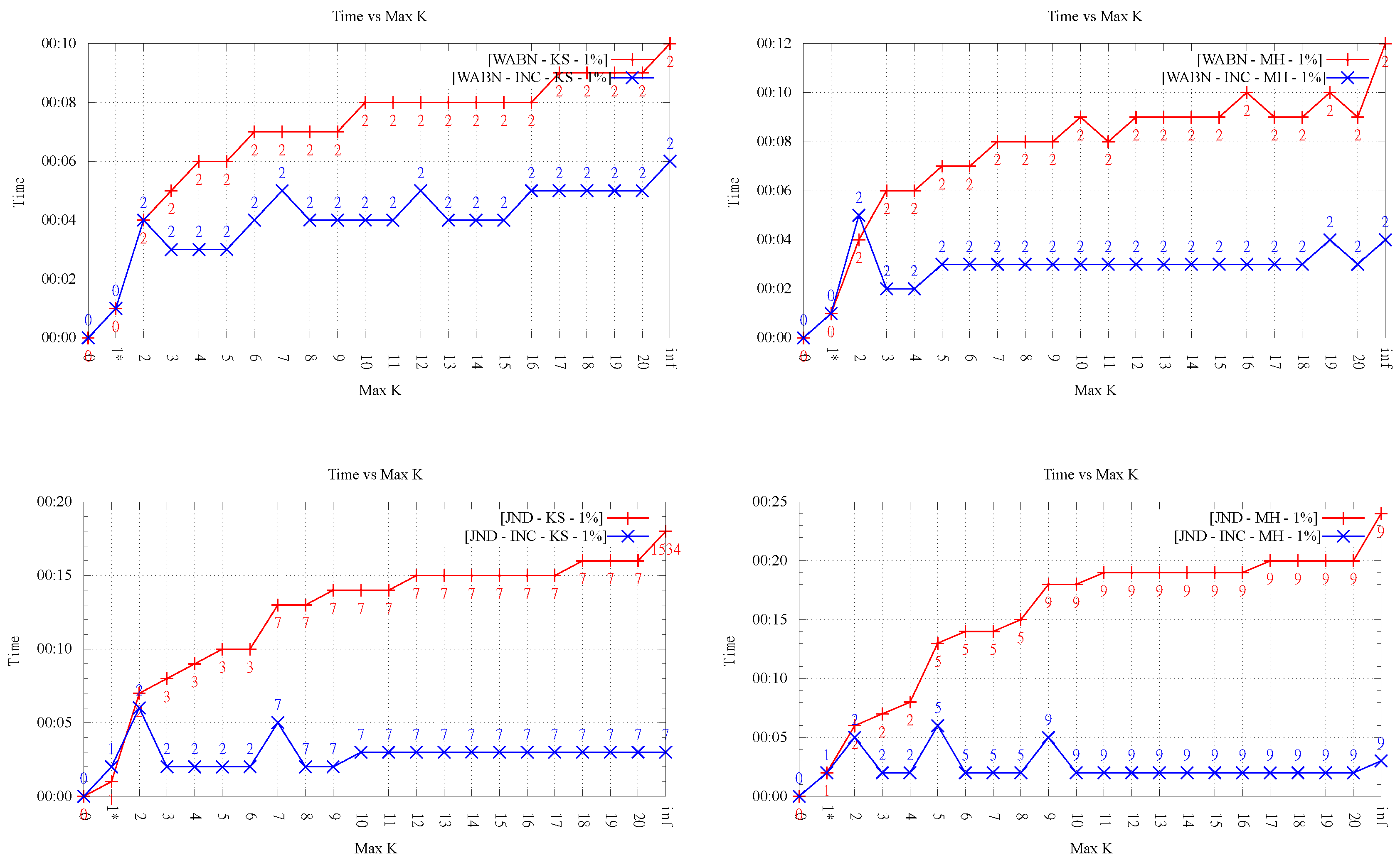
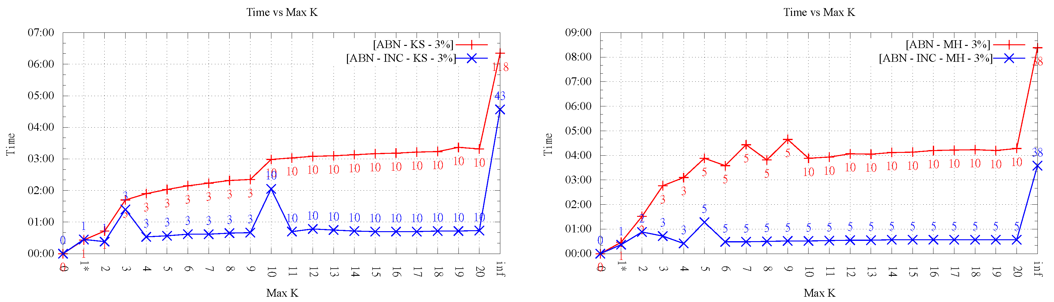
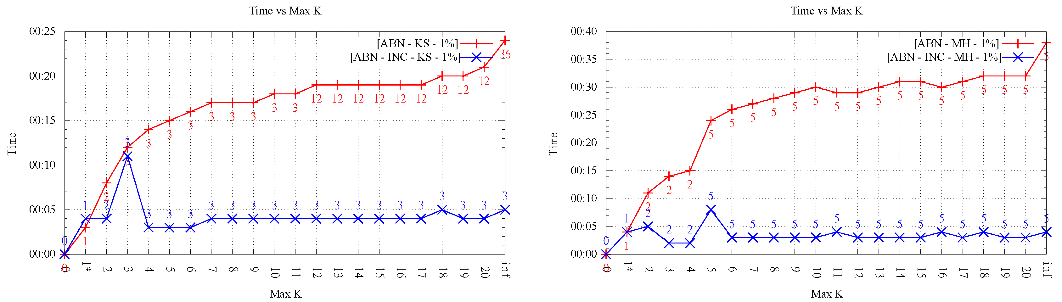
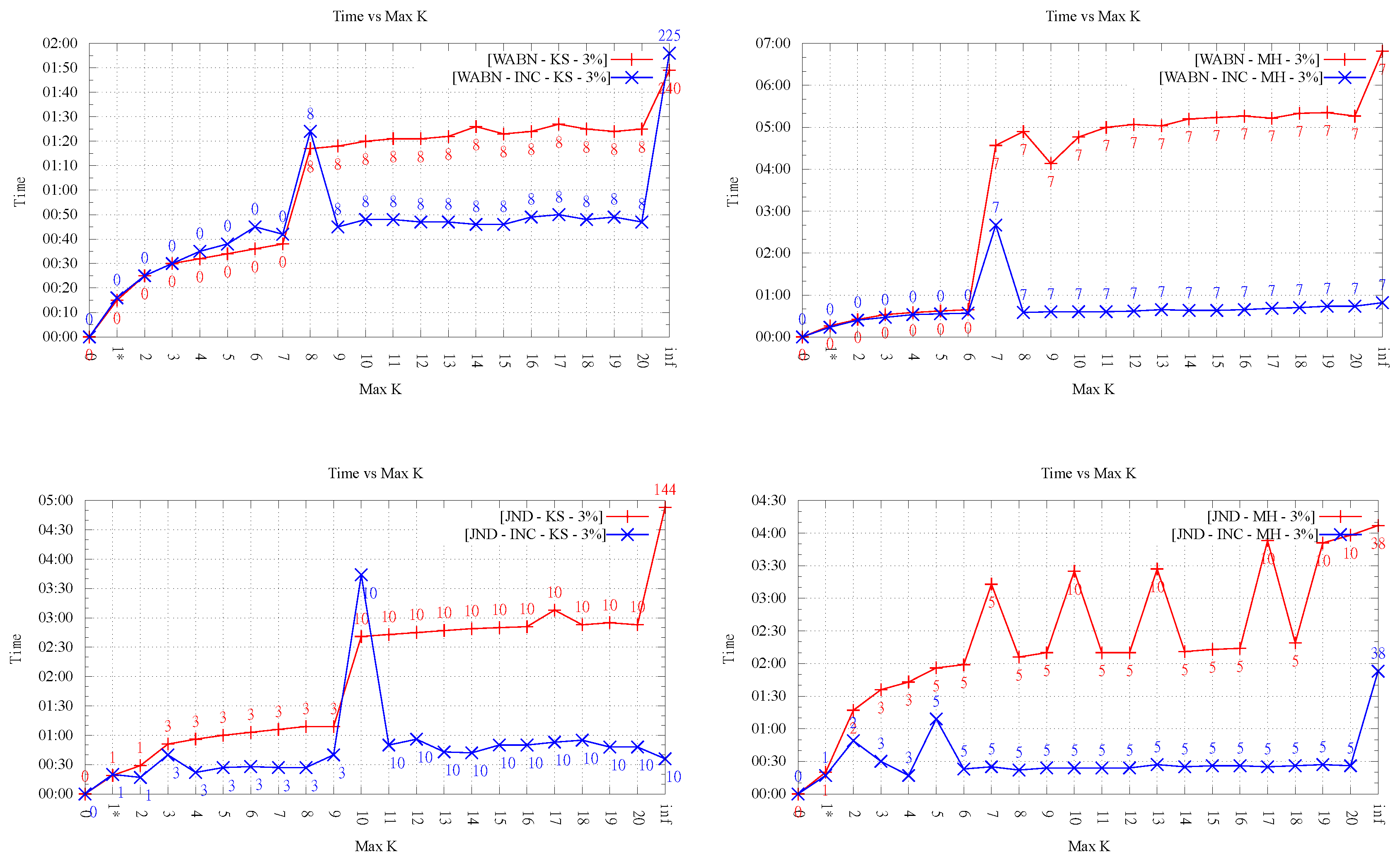
4.5. Running Time for
In this section, we analyze the running time as the order k increases. As mentioned before, our implementation was not optimized, thus it is not the actual time values but the overall behavior that is interesting to observe.
Figure 8 and
Figure 9 show an important growing trend of runtime as a function of
k. Even though the growing trend is very clear, the absence of monotonicity in the plot of LOP-0 is explained, again, by the fact that different orders behave independently and can result in very different flips. It is clear from these experiments that, as
k increases, the search space of order-
k Delaunay triangulations increases considerably, involving higher running times.
Likewise, it is interesting to note that in all cases, order-k (for ) optimization was faster than . This shows that restricting the order gives always faster methods in comparison with the unconstrained LOP method (for both variants), as proposed in the original data-dependent literature.
It can also be observed a clear difference in behavior between the two LOP variants; while, for LOP-0, a growing trend of time is seen as order k increases, LOP-INC exhibits generally much lower values except for some peaks where the flips changing the final order of triangulation are performed. Thus, as expected, the running times registered by the executions of LOP-INC are considerably lower for LOP-0. Indeed, LOP-INC was faster in almost every run, with speed-ups of a factor between 2 and 9 for . This is explained by the fact that, for LOP-INC, the starting point of the k-ODT construction is the -ODT, resulting in less flips per execution and consequently less running time.
4.6. Comparison between ABN, WABN and JND
Although it is not the aim of this paper to determine which data-dependent measure is most suitable, a couple of remarks about them are in order. (In the following analysis, we only refer to the results obtained with of
k-OD LOP-0.) Perhaps the most interesting aspect to evaluate, as a way to compare the quality of the approximations obtained by each criterion, is the behavior between ABN, WABN and JND with respect to the error metrics. Here, we observe that in every case the behavior of WABN was different, presenting in general higher RMSE values. Regarding JND and ABN, their behavior was similar for Kinzel Springs and different for Moorehead SE. Another aspect one can observe is the average aspect ratio of the resulting triangles. In this respect, when comparing ABN and WABN,
Figure 10 shows that in the majority of cases WABN produced a lower average aspect ratio than ABN, as expected.
This behaviour was observed in both variants of the LOP method.
5. Conclusions
This work studied the practical use of higher order Delaunay triangulations as a tool to implement data-dependent triangulations. We consider that the results obtained answer, to a large extent, the questions posed at the introduction, suggesting that HODTs are indeed suitable for data-dependent triangulations.
The most important question was whether HODTs allowed for obtaining a significant improvement in the value of data-dependent criteria. In our experiments, it was shown that, even for low orders, improvements can be significant, even when restricted to very small orders like . In addition, restricting to such small orders has the advantage that the running time overhead, in comparison with using the Delaunay triangulation, is kept under control. In relation to the standard LOP (i.e., )—the most standard way to implement data-dependent triangulations—our experiments suggest that LOP does not give any important benefit over k-OD LOP for low orders. On the contrary, LOP takes longer to run (at least 50% longer for the 1% data set and 35% longer for the 3% data set, in comparison with k-OD LOP for ), and may produce more slivers and higher approximation error.
The average aspect ratio does not seem to get significantly worse for the orders tested. In fact, for very small orders (e.g., ), there is no discernible difference. This is in contrast with the case , for which, as expected, the average aspect ratio got worse in most cases (although the difference in the average was, in general, rather small).
The implementation of the exact method for revealed several interesting aspects. Especially noteworthy is the fact that k-OD LOP always matched the optimal solution. This is encouraging, and shows that even though the theory can suggest that optimizing over may be intractable, in practice simple methods like k-OD LOP may give very acceptable solutions. On the other hand, 1-exact-KLS and 1-exact-DT ran in the majority of cases faster, although for practical use it seems better to use 1-exact-DT, which gives priority to Delaunay edges, due to the notably better RMSE values obtained.
Of the two variants of LOP implemented, LOP-INC showed in general advantages over LOP-0:
a lower final order of triangulations,
fewer flips,
monotonically decreasing values,
and—probably the most important difference—considerably faster.
Thus, from a practical point of view, it seems that, for an exploratory use of HODTs where many values of k want to be tested, LOP-INC is highly preferable.
Regarding the practicality of implementing HODTs, the k-OD LOP method resulted almost as simple as LOP-0, requiring only minimal additions to be able to compute the order of a triangle. The exact algorithm implementation was a bit more complex and required the use of an external library for SAT solving, but still can be considered a practical method, especially given its speed and that for almost all tests resulted in improvements.
Finally, in [
1,
2,
3,
4,
5,
6], it was argued that the improvement of methods based on minimization of curvature often gave improvements in the RMSE. However, in our experiments, this is not entirely clear. The RMSE results obtained for the three data-dependent measures show only a mild improvement in approximation error. Our experiments achieve significant improvements in the maximum ABN, but not always accompanied by improvements in the RMSE. Even though it was never the goal of this work to question the different data-dependent criteria, it does raise the question of whether these data-dependent criteria can improve significantly the approximation error for real terrains, or whether other criteria should be explored further. In any case, it seems that HODTs will be a useful tool to optimize data-dependent criteria in general.
We consider that the main pending issues for future work are: (1) exploring further whether some data-dependent measures, in combination with HODTs, can significantly improve the approximation error in relation to that of the Delaunay triangulation, and (2) making HODTs widely available to users (at least from a practical standpoint). In relation to (1), it is worth noting that the experiments presented in this paper are based on two real terrains, but as such they have the limitation of not covering many other types of terrains for which results may be different. It is therefore another interesting line of future research to extend these experiments to a wider family of terrains, preferably natural, that provide a more comprehensive sample of relevant terrain topographies. At this point, the use of synthetic terrains is also a valid option, as long as the selection and their design is justified in terms of geographic criteria (as opposed to the synthetic terrains used in previous work mentioned in
Section 2). As for (2), this work showed that a general optimization module based on local optimization is relatively easy to program; a good next step would be to make it available off-the-shelf in some of the major GIS, with the option of customizing the optimization criteria. Then, the users could decide by themselves whether HODTs and data-dependent triangulations can offer a better alternative to Delaunay.


