Article

Quantifying Tourist Behavior Patterns by Travel Motifs and Geo-Tagged Photos from Flickr

1
School of Geodesy and Geomatics, Wuhan University, Wuhan 430079, China
2
Institute of Remote Sensing and Geographical Information Systems, Peking University, Beijing 100871, China
3
School of Remote Sensing and Information Engineering, Wuhan University, Wuhan 430079, China
4
Department of Land Surveying and Geo-Informatics, The Hong Kong Polytechnic University, Hung Hom, Kowloon, Hong Kong, China
*
Author to whom correspondence should be addressed.
ISPRS Int. J. Geo-Inf. 2017, 6(11), 345; https://doi.org/10.3390/ijgi6110345
Submission received: 9 September 2017 / Revised: 4 October 2017 / Accepted: 2 November 2017 / Published: 7 November 2017

Abstract

:
With millions of people traveling to unfamiliar cities to spend holidays, travel recommendation becomes necessary to assist tourists in planning their trips more efficiently. Serving as a prerequisite to travel recommender systems, understanding tourist behavior patterns is therefore of great importance. Recently, geo-tagged photos on social media platforms like Flickr have provided a rich data source that captures location histories of tourists and reflects their preferences. This article utilizes geo-tagged photos from Flickr to extract trajectories of tourists and then extends the concept of motifs from topological spaces, to temporal spaces and to semantic spaces, for detecting tourist mobility patterns. By representing trajectories in terms of three distinct types of travel motif and further using them to measure user similarity, typical tourist travel behavior patterns associated with distinct sightseeing tastes/preferences are identified and analyzed for tourism recommendation. Our empirical results confirm that the proposed analytical framework is effective to uncover meaningful tourist behavior patterns.

1. Introduction

Nowadays, millions of people prefer traveling to another city to spend holidays. To navigate in an unfamiliar tourism destination (e.g., city or region), tourists usually visit its famous attractions via the popular travel routes. However, the popularity of attractions and travel routes is time-evolving and depends on many factors, such as seasons, time budgets and personal preferences. Consequently, the latest and most effective recommendations need to be explored for tourists to elevate the satisfaction and experience of their journeys.
In existing tourism studies, travel recommendation for tourists is generally classified into two categories: generic and personalized [1]. The generic travel recommendation follows the paradigm of “trajectories → interesting locations → popular travel sequences → itinerary planning → activities recommendation” [2]. In comparison, a personalized recommender offers locations matching an individual’s preferences, which are learned from the individual’s location history [3]. To achieve the goal, a variety of methods is adopted to acquire people’s travel data, such as surveying tourist’s location histories [4] and automatic location-sensing devices like global positioning systems (GPS) [5]. The cost, scalability and privacy issues, however, hinder the effectiveness of these methods. Promisingly, social media platforms, such as Flickr, Twitter, Facebook, OpenStreetMap, etc., enable users to share their tourism-related information [6,7]. In reality, the fact that users prefer to use social media apps, particularly photo sharing services, during tourism activities has been widely recognized [8,9]. Those photo-sharing services have already led to enormous community-contributed photos with text tags, timestamps and geographic references on the Internet. More importantly, it turns out that the geo-tagged photos can tackle the aforementioned issues in previous methods and provide an effective solution to automatic tourist mobility analysis [10].
As the most popular photo-sharing platform, Flickr has accumulated a large collection of photos with metadata (such as location, time, size, camera type with which each photo was taken) and textual information (such as title, tag, etc.) that partially capture individuals’ travel activities in space and time [11]. These geo-tagged photos have been widely used to re-construct trajectories of tourists and to uncover the underlying tourist behavior patterns [12]. With the assistance of geo-tagged photos from Flickr, significant advances have been achieved for our understanding of tourists’ travel behavior patterns. For instance, Pladino et al. quantified both the global and local attractiveness of several famous tourism destinations using information from geo-tagged photos [13]. Arase et al. identified people’s frequent trip patterns, i.e., typical sequences of visited cities and stay durations, as well as descriptive tags that characterize the trip patterns [14]. They defined six trip themes (i.e., Landmark, Nature, Event, Gourmet, Business, Local) and mined frequent trip patterns on each theme at the city level. Nonetheless, much of the existing research only focuses on the city level of locations for photo trip mining, whereas the scene level is more informative. Hence, Lu et al. extracted popular travel routes from geotagged photos by clustering and took into account a number of factors such as duration of the trip and traveling cost to help the tourist with trip planning [15]. Zheng et al. investigated tourist’s movement patterns in relation to the regions of attractions and the topological characteristics of travel routes visited by different tourists [16]. Sun et al. built a recommendation system that provides users with the optimal travel routes, of which the basic unit is the separate road segment instead of the GPS trajectory segment [17]. Simply put, those exploratory investigations are making Flickr photograph data the most promising data source for tourism study in academic society.
From a methodological perspective, travel patterns and routes taken by tourists between main attractions are conventionally modeled by the Markov chain-based approach [18,19] or collaborative filtering [20,21]. It generally requires the detection of frequent travel sequences to gain a deep insight into the tourists’ travel behaviors. Recently, with the advance of complex network science, a tourist’s location history can be represented as a directed graph where a node is a location and an edge denotes the traveling sequence [22,23]. Popular travel sequences in those graphs can be termed as motifs in analogy to motifs in complex network, which were originally defined as patterns of interconnections occurring in complex networks at numbers that are significantly higher than those in randomized networks [24]. Jackson et al. systematically investigated motifs according to different shapes as feed-forward loop, chain, feedback loop, feedback with two mutual dyads, bi-fan, bi-parallel, fully-connected triad and uplinked mutual dyad [25]. Motifs were further classified as hub-and-spoke, pairs, trees, chains, triads, cycles and stars. It is also noteworthy that Kovanen et al. introduced the framework of temporal motifs to study classes of similar event sequences, where the similarity refers not only to network topology, but also to the temporal order of the events [26]. Stimulated by the aforementioned studies, Schneider et al. adopted the concept of motifs to study human mobility and found that only 17 unique motifs are present in daily mobility, which are sufficient to capture up to 90 percent of the population in surveys and mobile phone datasets for different countries [27]. Those previous studies have confirmed that motifs possess great potential for analyzing travel patterns.
However, generic motifs do not take place semantics into consideration. Conventional tourism recommendation systems heavily rely on popular/frequent travel sequences of a group of tourists [28]. Those sequences consist of a list of ad hoc attractions and cannot reveal the tastes/preferences of different kinds of tourism activities between users [29]. For instance, tourists may travel distinctively in terms of the number and the category of attractions. In a sense, the generic motif can be regarded as the highly abstract form of popular/frequent travel sequences. It models the travel preference between a given number of potential attractions [27]. Nonetheless, the generic motif does not takes spatio-temporal semantic information of the node and the edge of the underlying travel network into consideration [24]. As a result, it fails to model tourists’ travel preferences between different types of attractions (such as natural, cultural attractions, and so on). However, understanding the frequent travel sequence with and without place semantics is both important and has distinct implications for tourism recommendation [30]. For instance, under certain scenarios, tourists have to plan their itinerary by deciding which type of sites to visit with high priority, as well as the duration of their visitation according to their personal preferences and time budgets. The generic motif is only capable of suggesting a popular route between a given number of attractions and cannot address the requirements of the priority and the duration of visiting different kinds of attractions. Therefore, motifs with spatio-temporal semantics are an urgent need for detecting more specific travel behavior patterns to enhance the capability of existing travel recommender systems.
From this point of view, this research focuses on Flickr photos taken in New York and aims to mine tourists’ frequent travel patterns in the city. In Section 2, we extend the concept of network motifs to unveil the spatio-temporal semantics of different travel motifs and quantify user similarity based on topological, temporal and semantic travel motifs to distinguish users with different preferences for assisting travel recommendation. In Section 3, empirical results are described for our understanding of several typical tourists’ travel behavior patterns within the case study area. Section 4 discuss the limits and potentials of the proposed analytic framework. Section 5 highlights our contributions and concludes the paper.

2. Methods

2.1. Tourist Trajectory

Tourists usually visit several sightseeing venues, which are in general popular landmarks, at their tourism destination. In this sense, a tourist trajectory usually consists of a sequence of landmarks with spatial, temporal and semantic information.

2.1.1. Constructing Travel Trajectory

Given a set of n popular landmarks (or “places” in a general sense) L = { l 1 , l 2 , , l n } at a tourism destination, we denote the spatial and the semantic attributes of the i-th landmark as l i . g e o m and l i . t y p e . Under common circumstance, a tourist’s travel behavior is captured and recorded as a set of m points (i.e., geo-tagged and time-stamped photos) as P = { p 1 , p 2 , , p m } in space and time. For each point, its spatial and temporal information is explicitly logged in the form of p j . g e o m and p j . t i m e . As previously mentioned, it is informative to represent the tourist trajectory in terms of a sequence of landmarks ordered by the time that they are visited by the tourist. We therefore associate each point with its corresponding landmark and rewrite a tourist’s travel path T with explicit spatial, temporal and semantic attributes as follows:
T = { ( p 1 . t i m e , l 1 . g e o m , l 1 . t y p e ) , ( p 2 . t i m e , l 2 . g e o m , l 2 . t y p e ) , , ( p m . t i m e , l m . g e o m , l m . t y p e ) }
Note that there exist no duplicate landmarks l i . g e o m in L , and l i . t y p e is the type of landmark containing the geo-tagged photo p i . Since points in P may not match any landmarks in L , the condition will always hold as | | T | | m , where the operator | | | | counts the cardinality (i.e., the number of elements) of the input set.

2.1.2. Differentiating Natives and Tourists

Considering that tourists’ behavior is the scope of this research, photos uploaded by natives should be filtered out of further analysis. To put it simply, it is necessary to distinguish between tourists and natives based on their travel paths in space and time. Under common circumstances, a tourist stays in a tourism destination, for instance a city, within a short-term time period (e.g., one week). It is reasonable to assume that as for a tourist, his/her travel time T . t i m e is usually within the same month or at most two consecutive months, whereas a native can take photos in the target city in almost all months. As a result, travel time of a native is much more randomly distributed than that of a traveler, which leads to a native having a higher temporal entropy from a probabilistic perspective. Based on the above observation, we therefore apply an entropy-based filtering method to differentiate tourists from natives as:
f ( k ) = d a y s ( k , T . t i m e ) k = 1 12 d a y s ( k , T . t i m e )
E = k = 1 12 f ( k ) log f ( k )
where operator d a y s ( k , ) counts the total number of days on which an individual has photo records in the k-th month in the target region. Obviously, the higher the temporal entropy is, the higher the likelihood of the user to be a native. It is noteworthy that a suitable threshold ϵ e is needed to separate the native group and the traveler group. More specifically, an optimal threshold should, on the one hand, be low to make sure that there exist no natives among users with entropy less than the value. On the other hand, the number of users satisfying the threshold condition should be large for producing aggregate travel behavior patterns, which means that an optimal threshold should not be too low.

2.1.3. Segmenting Individual Travel Journey

As denoted in Equation (1), a tourist’s travel trajectory can be represented as a sequence of semantic photos in a concise form as:
P ¯ = { ( p ¯ 1 . t i m e , p ¯ 1 . g e o m , p ¯ 1 . t y p e ) , , ( p ¯ s . t i m e , p ¯ s . g e o m , p ¯ s . t y p e ) }
where ( p ¯ 1 , , p ¯ s ) are the photos falling within a landmark, and if consecutive photos are attached to an identical landmark, we can obtain the tourist’s duration of stay at this landmark and further rewrite the travel path as:
P ¯ = { ( p ¯ 1 . t i m e , p ¯ 1 . g e o m , p ¯ 1 . t y p e , p ¯ 1 . d u r a t i o n ) , , ( p ¯ u . t i m e , p ¯ u . g e o m , p ¯ u . t y p e , p ¯ u . d u r a t i o n ) }
Obviously, the condition meets u s m . Moreover, a tourist’s travel trajectory usually consists of several separate travel journeys, which are not continuous in time. Due to this fact, we therefore develop two steps of criteria to segment each tourist’s travel trajectory into individual travel journeys based on the interval ϵ t between two visited landmarks and the entire length ϵ l of a single journey as:
  • Criterion I: It is intuitive that a tourist seldom takes no photos in ϵ t consecutive days during a trip. If this situation happens, it is highly possible that the tourist pays another visit to the target city. In this sense, we segment tourists’ travel trajectories into distinct journeys if the time interval between two consecutive semantic photos exceeds a predefined ϵ t days. Mathematically, if ( p ¯ i + 1 . t i m e p ¯ i . t i m e ) ϵ t , we break the travel path into different parts.
  • Criterion II: Journeys are abandoned if the total duration of staying at the tourism destination is less than ϵ l minutes. Mathematically, if ( p ¯ e n d . t i m e p ¯ s t a r t . t i m e ) ϵ l , we drop this journey from further analysis.
As a result, each tourist is associated with a set of travel journeys that are organized in the form of distinct landmarks and connections between them. Put more straightforwardly, a journey can be regarded as a directed spatial network that contains implicit spatio-temporal information of tourists’ travel behaviors.
J = { ( p ¯ s t a r t . t i m e , p ¯ s t a r t . g e o m , p ¯ s t a r t . t y p e , p ¯ s t a r t . d u r a t i o n ) , , ( p ¯ e n d . t i m e , p ¯ e n d . g e o m , p ¯ e n d . t y p e , p ¯ e n d . d u r a t i o n ) }
P ¯ = { J 1 , J 2 , , J v }

2.2. Travel Motif

Many systems represented as complex networks consist of various sub-networks, either topological or temporal. If these sub-networks occur more often than in randomized versions of the entire network, these sub-networks are called motifs. Put simply, network motifs are sub-graphs that repeat themselves in a specific network or even among various networks. Each of these sub-graphs, defined by a particular pattern of interactions between vertices, may reflect a framework in which particular functions are achieved efficiently. It is well-received that motifs are of notable importance largely because they may reflect functional properties and provide deep insight into the network’s functional abilities. They have recently gathered much attention as a useful technique for uncovering structural design principles of complex networks.

2.2.1. Topological Travel Motif

In the context of tourism study, topological travel motifs refer to sub-graphs in mobility networks that describe trip patterns without considering specific place semantics. Particularly, Schneider et al. proposed that the “daily network” of visited locations, in which nodes represent the visited locations and directed edges stand for trips between them, can be taken as the travel motif and reveals the underlying individual mobility patterns [27]. In this research, we argue that this generic definition discards important spatio-temporal characteristics of tourists’ travel behaviors and therefore propose two alternative definitions for quantifying topological characteristics of their mobility patterns. Note that differences between Schneider’s and the proposed two motifs are discussed in Section 4.
Definition 1.
Schneider’s topological motif: The daily and the aggregated profiles of a given travel journey J = { p ¯ s t a r t , , p ¯ e n d } are directly described as a topological motif by discarding any additional information about the purpose of the activity, the travel time and the activity duration, as well as the distances and the number of trips between the visited locations. To be concise, we denote this transformation as an operator Λ ( ) . In this sense, Schneider’s topological motif is Λ ( J ) .
Definition 2.
Discrete topological motif: For a given travel journey J = { p ¯ s t a r t , , p ¯ e n d } of length | | J | | = n , its subsequence X = { p ¯ i , , p ¯ j , , p ¯ k } of length | | X | | = m , i.e., X J and i < j < k , can be extracted. Note that there are C n m subsequences of length m, and those visited locations in X are not consecutive in the order of the original sequence in J . For simplicity, discrete topological motif can be formed as Λ ( X ) .
Definition 3.
Consecutive topological motif: For a given travel journey J = { p ¯ s t a r t , , p ¯ e n d } of length | | J | | = n , its consecutive subsequence Y = { p ¯ i , , p ¯ i + m 1 } of length | | Y | | = m , i.e., Y J , can be extracted. Note that there are ( n m + 1 ) subsequences of length m, and those visited locations in Y are consecutive in the order of the original sequence in J . For simplicity, the consecutive topological motif can be formed as Λ ( Y ) .
It is noteworthy that, because randomized versions of the mobility networks are not feasible and not all motifs are significant, in this research, we further filter out motifs that are found on average no more often than ϵ m percent in the datasets. With the predefined operator Λ ( ) , two travel sequences S 1 and S 2 will be assigned to the same motif, i.e., Λ ( S 1 ) = Λ ( S 2 ) , even though their corresponding nodes in S 1 and S 2 stand for different places. Mathematically, if two travel (sub-)networks belong to an identical motif, their adjacency matrices must be the same through certain sets of line and column transformations, and vice versa [27].

2.2.2. Temporal Travel Motif

The topological travel motif demonstrates that tourists travel according to different topological travel patterns given a certain number of locations. Another interesting research question is whether tourists travel following distinctive temporal patterns. For a given topological travel motif with m locations, staying times at different locations are usually not equal to each other. For instance, given a cycle motif with three nodes Λ ( { p ¯ 1 , p ¯ 2 , p ¯ 3 } ) , some tourists spend the most time at the first place and much less time at the other two (i.e., p ¯ 1 . d u r a t i o n > p ¯ 2 . d u r a t i o n and p ¯ 1 . d u r a t i o n > p ¯ 3 . d u r a t i o n ), while other tourists may visit three places in roughly equal time portions (i.e., p ¯ 1 . d u r a t i o n p ¯ 2 . d u r a t i o n p ¯ 3 . d u r a t i o n ).
Based on the above observation, this study introduces temporal travel motifs as an additional dimension of tourists’ travel behaviors. Before classifying a topological travel motif Λ ( S ) of length m into one category of temporal travel motif, it is necessary to transform it into a K-node temporal sequence, where K m . To achieve this goal, we define the operator u n i q ( ) as the set of distinct locations { l o c 1 , l o c 2 , } in the topological motif,
u n i q ( Λ ( S ) ) = { l o c 1 , l o c 2 , }
where:
l o c i = { p ¯ a , p ¯ b , }
l o c i . d u r a t i o n = ( p ¯ a . d u r a t i o n + p ¯ b . d u r a t i o n + ) | | l o c i | |
and locations are ordered according to their first appearances in the travel sequence. Note that under most scenarios, there exists no overlap between two aggregated locations l o c i and l o c j , i.e., l o c i l o c j = { p ¯ a , p ¯ b , } { p ¯ c , p ¯ d , } = . Finally, we transform the topological motif into a temporal sequence T following the rules listed below:
  • If the given topological motif S contains less than K distinct locations (i.e., | | u n i q ( Λ ( S ) ) | | < K ), its corresponding temporal travel sequence is:
    T = { l o c 1 . d u r a t i o n , , l o c | | u n i q ( Λ ( S ) ) | | . d u r a t i o n , 0 , , 0 }
  • If the given topological motif S contains exactly K distinct locations (i.e., | | u n i q ( Λ ( S ) ) | | = K ), its corresponding temporal travel sequence is:
    T = { l o c 1 . d u r a t i o n , , l o c | | u n i q ( Λ ( S ) ) | | . d u r a t i o n }
  • If the given topological motif S contains more than K distinct locations (i.e., | | u n i q ( Λ ( S ) ) | | > K ), its corresponding temporal travel sequence is:
    T = { l o c 1 . d u r a t i o n , , l o c K 1 . d u r a t i o n , l o c K . d u r a t i o n + + l o c | | u n i q ( Λ ( S ) ) | | . d u r a t i o n | | u n i q ( Λ ( S ) ) | | K + 1 }
    which means that the staying time of the K-th location is replaced by the average of staying times from the K-th location to the last location.
Based on the above definition, each topological travel motif is transformed into a K-node temporal sequence (i.e., l o c 1 l o c 2 l o c K ), which is further classified into one type of temporal travel motif that is defined according to the relationship of staying time in K distinct nodes.

2.2.3. Semantic Travel Motif

Since sightseeing preferences vary among tourists, tourists’ visiting orders of different types of attractions (e.g., landmarks in this research) can also differ. Generally speaking, a tourist tends to visit his/her favorite attraction sites first and then go to see other attractions of less interest later. This phenomenon implies that the visiting order of tourism attraction sites enables us to explore tourists’ travel and sightseeing preference, and a group of similar sequences of attractions stands for a cluster of tourists with resembling tastes.
There are two factors that determine the similarity of two travel sequences between landmarks: one is the semantic closeness of the landmarks, and the other is the alignment of different semantic types of landmarks. Formal rules for attaching semantic characteristics to a travel motif are listed below:
  • Regarding the first factor, landmarks are classified into L distinct categories, where landmarks in each category are semantically homogenous on the basis of common sense [31]. In this way, a semantic topological travel motif can be transformed into an L-type semantic-category sequence. For instance, “The Museum of Modern Art → Bryant Park → Times Square” is represented as “Cultural → Business → Natural”. In this sense, a semantic travel sequence C is formally defined as:
    (14) C = { c 1 , c 2 , , c k } (15)       = { l o c 1 . t y p e , l o c 2 . t y p e , , l o c k . t y p e }
    where c i denotes the semantic category of the i-th location.
  • With regard to the alignment of different semantic types of landmarks, the semantic travel motif is generated by the relative value of each category of attractions. Here, we define the value as the average of subscripts of categories that are identical to the target category in a semantic travel sequence and denote it by the operator r a n k ( ) as:
    r a n k ( c ) = r a n k ( c i ) n , if c i = l o c i . t y p e = c and there exists n such locations in C + , if there exists no locations associated with category c
Put straightforwardly, if there exists no such category in the travel sequence, its semantic value is assigned to be infinitely large. As a result, a smaller value of a given category indicates that landmarks pertaining to this category are preferred by tourists. An infinite value means that the priority of visiting the corresponding landmark is minimized.

2.3. Motif-Based Clustering

Given a user’s travel trajectories, the corresponding topological travel motifs, temporal travel motifs and semantic travel motifs are derived. Then, each trajectory is denoted by three types of motifs in terms of a feature vector. Based on the resultant vector, the similarity between two users can be directly measured. The input of the clustering process is the travel trajectories of two users, and the output will be a similarity score indicating how similar these two users are. Note that this proposed clustering framework is not applied to users who visit only one place since a one-node motif does not belong to any of the defined categories of motifs.
To attach auxiliary information to topological travel motifs, we further assign those resultant motifs to λ categories based on their topological morphologies as “chain”, “cycle”, “downlinked mutual dyad”, “uplinked mutual dyad”, and so on. Recall that the temporal and the semantic travel sequences are ordered to reveal tourists’ sightseeing preferences; we also assign them to a couple of categories, γ for temporal motifs and δ for semantic motifs, based on the duration pf stay and the visitation order at each landmark. By doing so, we finally obtain a set of vectors that denote what type of topological, temporal and semantic travel motifs a tourist’s travel journey belongs to, respectively:
W = { w o 1 , w o 2 , , w o λ 1 , w o λ , w t 1 , w t 2 , , w t γ 1 , w t γ , w c 1 , w c 2 , , w c δ 1 , w c δ }
where the length of W is ( λ + γ + δ ) ; each element stands for one category of motifs, and elements that represent motifs the trajectory pertains to are assigned to be one and all others zero. Furthermore, given a user who has n individual travel journeys, his/her travel behavior R is represented by adding up all W s as:
R = W 1 + W 2 + + W n n
In this way, each user is represented by a ( λ + γ + δ ) -element vector. Given users’ vectors, we further adopt the cosine of the angle between two vectors (i.e., “cosine similarity”) as the similarity score of two users a and b :
S i m ( a , b ) = R a · R b | R a | · | R b |

3. Data and Results

Geo-tagged photos analyzed in this research were downloaded from Flickr through its publicly available API, which are provided as part of the Yahoo! Webscope program for use solely under the terms of a signed Yahoo! Data Sharing Agreement [32]. For more details, readers can access this dataset online via https://webscope.sandbox.yahoo.com/catalog.php?datatype=i&did=67.

3.1. Yahoo Flickr Creative Commons 100M Dataset

The Yahoo Flickr Creative Commons 100M (YFCC100m) dataset contains a list of photos and videos that is compiled from data available on Yahoo! Flickr. Each record consists of a photo ID, a jpeg url or video url and some corresponding metadata such as the title, description, camera type and tags. Moreover, about 49 million of the photos are geo-tagged (see Figure 1 as an illustration), which enables us to explore human mobility patterns of the corresponding users in space and time. More specifically, each geo-tagged photo, which is utilized for this research, has the following attributes: photo ID, user ID, date taken, longitude, latitude, accuracy, title, user tags, machine tags, etc.
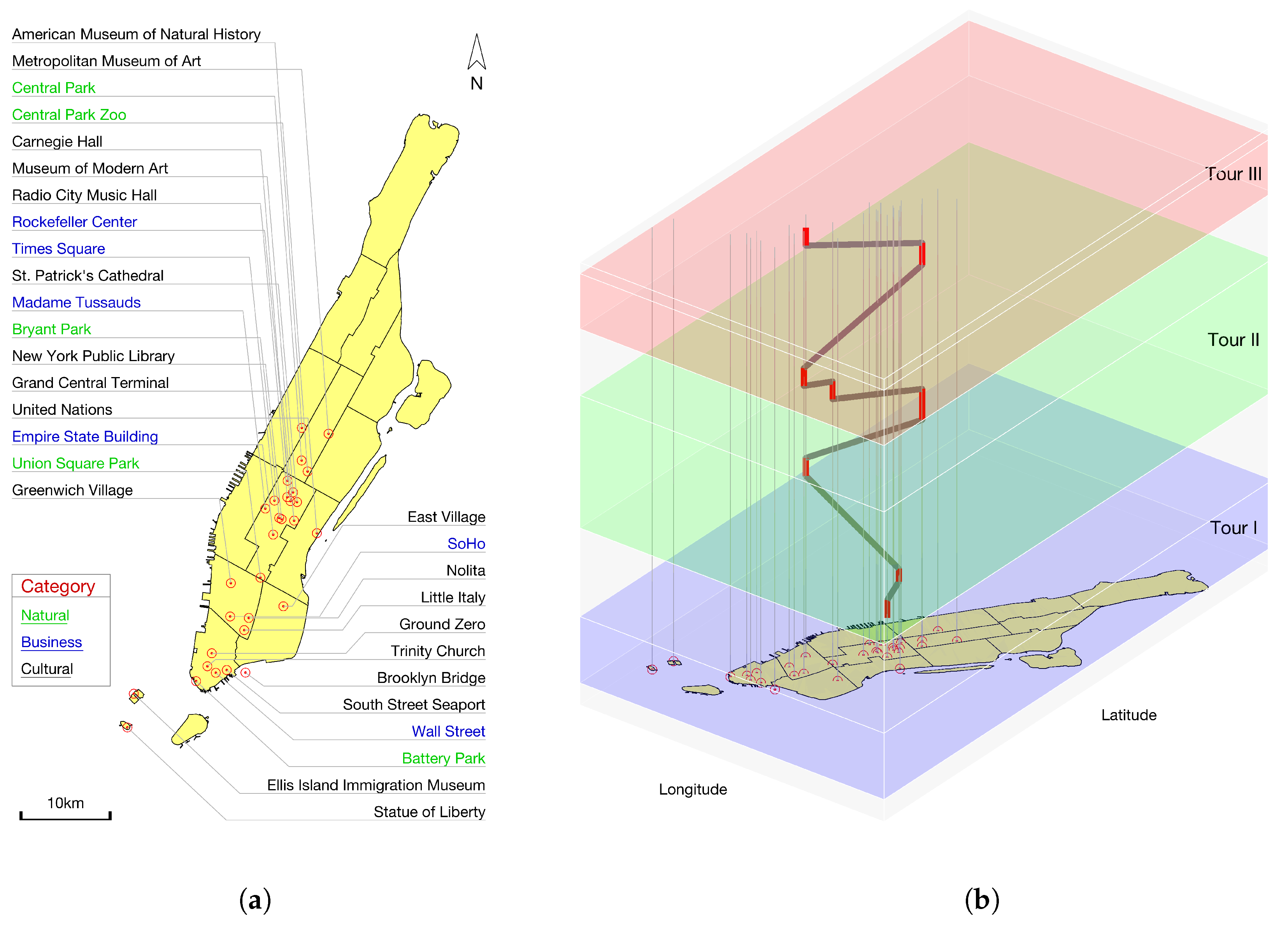
In this research, we concentrate on city-scale tourism mobility and select Manhattan Island of New York City, which is one of the hottest tourism destinations worldwide, as the case study area (see Figure 2a). In order to find users who have visited the top 30 landmarks in Manhattan, we firstly select photos taken in this target region according to their longitude and latitude. Thereafter, the user ID associated with those photos is extracted, and the corresponding complete photo collections of these users are derived. Following the procedures introduced in Section 2.1, we finally obtain 2622 travel trajectory journeys of 2184 tourists for travel motif and mobility pattern analysis. It is noteworthy that we run several trials to extract tourist trajectories, and the optimal parameters are: temporal entropy ϵ e = 0.7 , journey interval ϵ t = 5 , journey duration ϵ l = 10 . Additionally, tourists with less than 10 photos taken within the case study area are excluded as their shared geo-tagged photos are too sparse in space and time to construct reliable travel trajectories.
Positioning those resultant tourists’ geo-tagged photos with respect to the selected 30 landmarks, we can intuitively unveil the popularity of each landmark based on its tourist traffic volume, namely the number of people that have taken photos in the region, as well as its traffic duration, namely the length of time spent by tourists at the landmark. Results indicate that: (1) the top five landmarks that attract more tourists than those of the others are “Central Park” (1306), “Rockefeller Center” (632), “Greenwich Village” (614), “Empire State Building” (494) and “Brooklyn Bridge” (415); (2) the top five landmarks that gain more from the time budget of tourists than the others are “Greenwich Village” ( 2.75 h), “Carnegie Hall” ( 2.71 h), “SoHo” ( 2.63 h), “Little Italy” ( 2.48 h) and “American Museum of Natural History” ( 2.36 h). Interestingly, “Greenwich Village” is the only landmark existing in both types of top five landmarks, indicating that it is a very popular tourism destination within the case study area. Besides, there are a limited number of tourists visiting museums and music halls, but once visiting there, tourists spend much time on them. A typical example is “Carnegie Hall”, which is a well-known concert venue. There are only eight tourists visiting it, but the average time spent there is 2.71 h. A similar situation happens to “SoHo”, which is a grand shopping destination with flagship stores of famous brands. Even though tourists spend a similar length of time in “Carnegie Hall” and “SoHo”, it can be assumed that travelers to these two places should have different tastes. Another interesting observation is that there are only five people traveling to the “Statue of Liberty”, which is a world-famous landmark and thus should have attracted an enormous amount tourists like “Central Park”. The reason why a part of the tourists miss it is that it is only accessible by ferry and not easy to work into trips. Besides, the best position for taking a picture of the “Statue of Liberty” is “Battery Park”, rather than the statue itself. Nevertheless, overall, the number of visitors and time spent in different tourism sites can reflect their popularity and provide tourists with a reference to plan trips when they visit Manhattan Island, New York.

3.2. Typical Travel Motifs in Manhattan

Observing the travel paths between the top 30 landmarks (see Figure 2b as an example), we identify 22 directed edges that are frequent routes preferred by a large number of tourists. A typical feature that these edges have in common is that 10 out of them have “Central Park” as either the “source” node or the “sink” node, which implies that “Central Park” is a central tourism destination, and tourist traffic tends to flow from several other landmarks to it or depart from it to other landmarks. This discovery is consistent with the high outdegree/indegree of “Central Park”. On both a personal and a daily basis, there are three routes (i.e., “Central Park → Metropolitan Museum of Art”, “Rockefeller Center → Central Park”, “Central Park → Rockefeller Center”) that turn out to be popular. Results also show that “Greenwich Village → Central Park” and “Empire State Building → Central Park” in personal trips cover much longer distances than those of “Central Park → American Museum of Natural History” and “Metropolitan Museum of Art → Central Park” in person-day trips. This can be explained as tourists tend to visit “Greenwich Village” (or “Empire State Building”) as the final destination in a day and “Central Park” as the first venue the next day.
In order to find out frequent travel patterns, this study labels a unique sub-network as a motif only if it occurs more often than ϵ m = 5 percent in the dataset. Specifically, for the 2622 derived trajectories in the resulted dataset, the threshold for maintaining a motif is: 2622 × 5 % = 131 , which suggests that a motif should be a pattern that at least 131 tourists follow. Note that we extracted travel motifs under different thresholds, i.e., ϵ m % = 0.01, 0.02, 0.03, 0.04, 0.05, and so on, and selected 0.05 as the optimal threshold in that the resultant motifs covered a significant part of tourists and were easy to interpret. Based on the above principles, 13 motifs are discovered to be capable of describing up to 87.4 percent of all trips in the dataset. For the temporal travel motifs, we concentrate on the first K = 3 distinct landmarks of tourists’ travel journeys for the sake of conciseness. For the semantic travel motifs, we adopt a division of landmarks with L = 3 types of categories termed as {“natural”, “business”, “cultural”}. In the context of this research, the “Natural” category mainly consists of parks, while “Cultural” places includes museums, libraries, historic sites, and so on. The “Business” type represents business districts like “Wall Street” and “Rockefeller Center”. Note that alternative and better accuracy division of categories instead of the one as shown in Figure 2a can be utilized for this analysis. Under those experimental settings, we consequently obtain a collection of typical topological, temporal and semantic travel motifs, respectively.

3.2.1. Characteristics of Topological Travel Motifs

As illustrated in Figure 3a,b, topological travel motifs are ordered by their sizes and their frequencies of occurrences from left to right. Given the predefined threshold ϵ m = 5 , the number of locations that these detected motifs contain ranges from 1–6 for both discrete and consecutive topological motifs. Statistically, most tourists visit only one landmark in the case study area. The next likely motif is a point-to-point pattern (ID = 2), followed by the motif with three locations and two tours (ID = 4). Actually, apart from the one-location motif (ID = 1), motifs with n locations and ( n 1 ) tours account for the largest part of the overall patterns (ID = 2, 4, 9, 16, 26 for the discrete topological motif and ID = 2, 4, 8, 12, 13 for the consecutive topological motif).
From top to bottom, topological travel motifs are categorized into λ = 5 types based on their morphologies as: {“chain”, “cycle”, “downlinked”, “central linked”, “uplinked”}. Note that the one-node motif (ID = 1) is excluded from these categories. As previously mentioned, those “chain” motifs conform to common travel patterns such that tourists visit places one by one like a chain and without turning back. As a comparison, all remaining motifs have n locations and n tours. Nonetheless, these motifs are still different in terms of structure. For instance, “downlinked mutual dyad” refers to a motif such that the “mutual dyad” is visited ahead of the “chain”, while it comes later than the “chain” in “uplinked mutual dyad”. On average, motifs in a “circle” shape (ID = 3, 5) occur more often than the others (such as ID = 6, 7). This kind of motif in a “circle” shape represents tourists who access a set of different places one by one and return to the starting location in the end. There are also tourists who return to the initial location after visiting a single place and then continue to travel to other places like a “chain” (ID = 6). It can be deduced that the single place is located far from the direction, or at least not the close direction of the later “chain” of places. Interestingly, a part of tourists follow the motif (ID = 7) that is a nearly “opposite” pattern to motifs with ID = 6, because they visit a chain of sites until the end and then return to the former site. Despite the sequential difference between ID = 6 and ID = 7, a common feature is that they all have one “central” location, defined as a node with more than two directed edges. The presence of a unique central node ensures that multiple tours along the same directed edge are suppressed. Hence, the edges of the motifs belong to exactly one tour, and all directed edges are visited exactly once. This conclusion is consistent with the common sense that tourists would not repeat a tour several times concerning the time budget. As for the functionality of the central location, the most possible one is accommodation that is just near a major tourism site. It is also observed that a landmark has different types of activities fixed at certain times so that travelers visit it in the morning to see its day-time scenery and return to it to experience another activity that is only available in the evening.
To summarize, tourists’ topological travel motifs demonstrate that their number of visited landmarks during a single journey are largely limited. More importantly, tourists usually visit several landmarks in a fashion as either one by one or with an anchor point. These findings will enable us to develop reliable travel recommendations for tourists in a general sense.

3.2.2. Characteristics of Temporal Travel Motifs

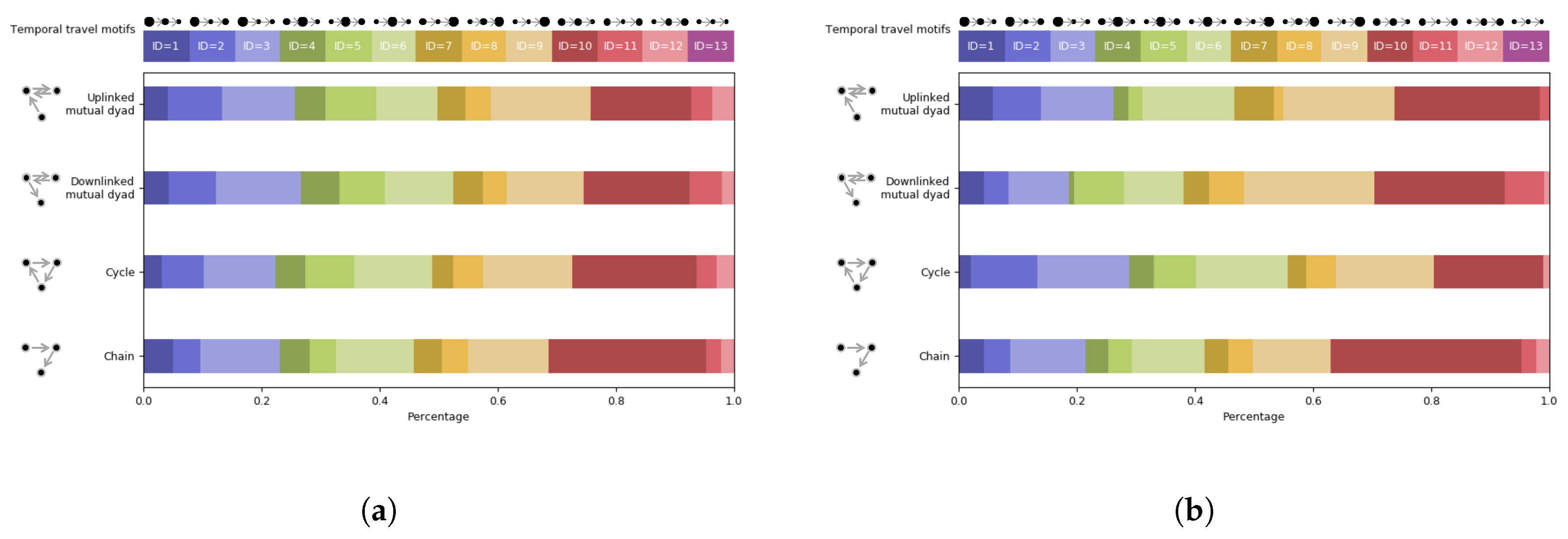
Temporal travel motifs denoted by the first K = 3 landmarks are illustrated in Figure 4a,b. Based on the duration of stay at these three locations, temporal travel motifs are assigned to γ = 13 categories as: { “⚫→ ”, “⚫→ ”, “⚫→ ”, “ →⚫→ ”, “ →⚫→ ”, “ →⚫→ ”, “ ”→ →⚫”, “ →⚫”, “ →⚫”, “ ”, “ ”, “ ”, “ ”} , where the size of the filled circle shows the relative duration of its staying time at each location. Note that we take durations of stay of two landmarks as the same order if they differ in less than 10 min. Besides, the blue series (ID = 1, 2, 3) denote motifs having the first place with the longest staying time, whereas the green series (ID = 4, 5, 6) for the second place, the brown series (ID = 7, 8, 9) for the third place and the other color series (ID = 10, 11, 12, 13) for other patterns.
For consecutive travel sequences, the common characteristic of tourists following “uplinked mutual dyad” and “cycle” is that they stay in the first place for the longest time (see Figure 4a). A slight difference between those two groups is that for “uplinked mutual dyad”, more tourists spend a longer time in the second place than the third place, compared with those pertaining to “cycle”. The third place takes the longest time for “downlinked mutual dyad” travelers, whereas travelers of the “chain” group show no preference for the index of the place with the longest duration. Besides, results show that for discrete travel sequences, the overall temporal travel patterns among those four types of topological motifs are similar (see Figure 4b). That is understandable since nodes in a discrete sequence are not necessarily consecutive, and hence, the relationship of their time durations is random, which results in a similar temporal travel pattern of four types of topological motifs. Apart from the above typical features, it is also obvious that even if tourists follow an identical topological travel motif, their temporal travel motif can be remarkably different. In other words, as a complementary metric, the duration of stay at different landmarks during a travel journey can well uncover tourists’ distinct travel preferences.

3.2.3. Characteristics of Semantic Travel Motifs

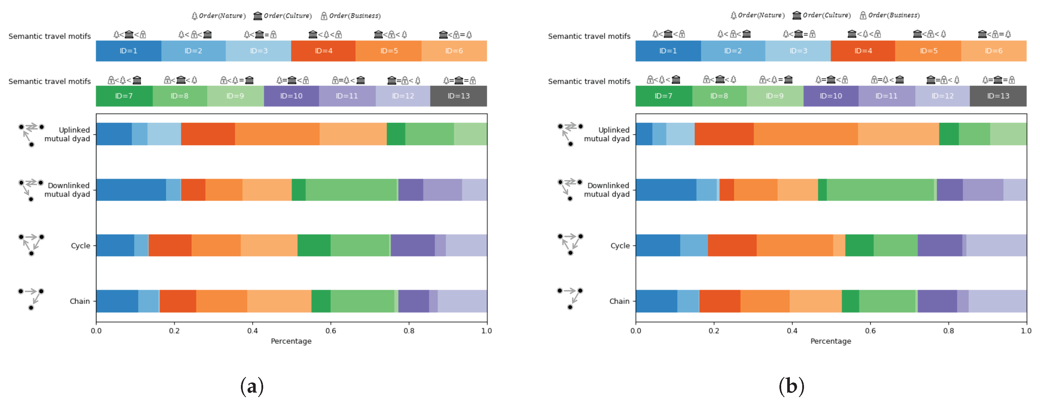
As illustrated in Figure 5a,b, dominant semantic travel motifs are quite different for topological travel motifs associated with distinct structural morphologies (please refer to Figure 3). Recall that landmark semantics are represented in terms of L = 3 types of categories as {“natural”, “business”, “cultural”}. Based on the semantic ranking of each category of landmarks within tourists’ travel sequences, we identify δ = 13 categories of semantic travel motifs as: { “ Ijgi 06 00345 i001”, “ Ijgi 06 00345 i002”, “ Ijgi 06 00345 i003”, “ Ijgi 06 00345 i004”, “ Ijgi 06 00345 i005”, “ Ijgi 06 00345 i006”, “ Ijgi 06 00345 i007”, “ Ijgi 06 00345 i008”, “ Ijgi 06 00345 i009”, “ Ijgi 06 00345 i010”, “ Ijgi 06 00345 i011”, “ Ijgi 06 00345 i012”, “ Ijgi 06 00345 i013”} , where “ Ijgi 06 00345 i014” represents “natural” landmark, “ Ijgi 06 00345 i015” represents “business” landmark, and “ Ijgi 06 00345 i016” represents “cultural” landmark.
For “uplinked mutual dyad”, most people prefer to visit “cultural” attractions first. As a comparison, “business → cultural → natural” dominates the overall semantic travel patterns of tourists pertaining to “downlinked mutual dyad”. For “cycle” and “chain”, even though “cultural” attractions outperform “business” and “natural” slightly in tourists’ first choices, the preference for these three types of attraction is distributed relatively evenly, compared with that under the “mutual dyad” scenarios. In this sense, semantic travel motifs can unveil divergent sightseeing tastes and, thus, are capable of distinguishing different travel interests of tourists.

3.3. Tourists’ Distinct Travel Patterns

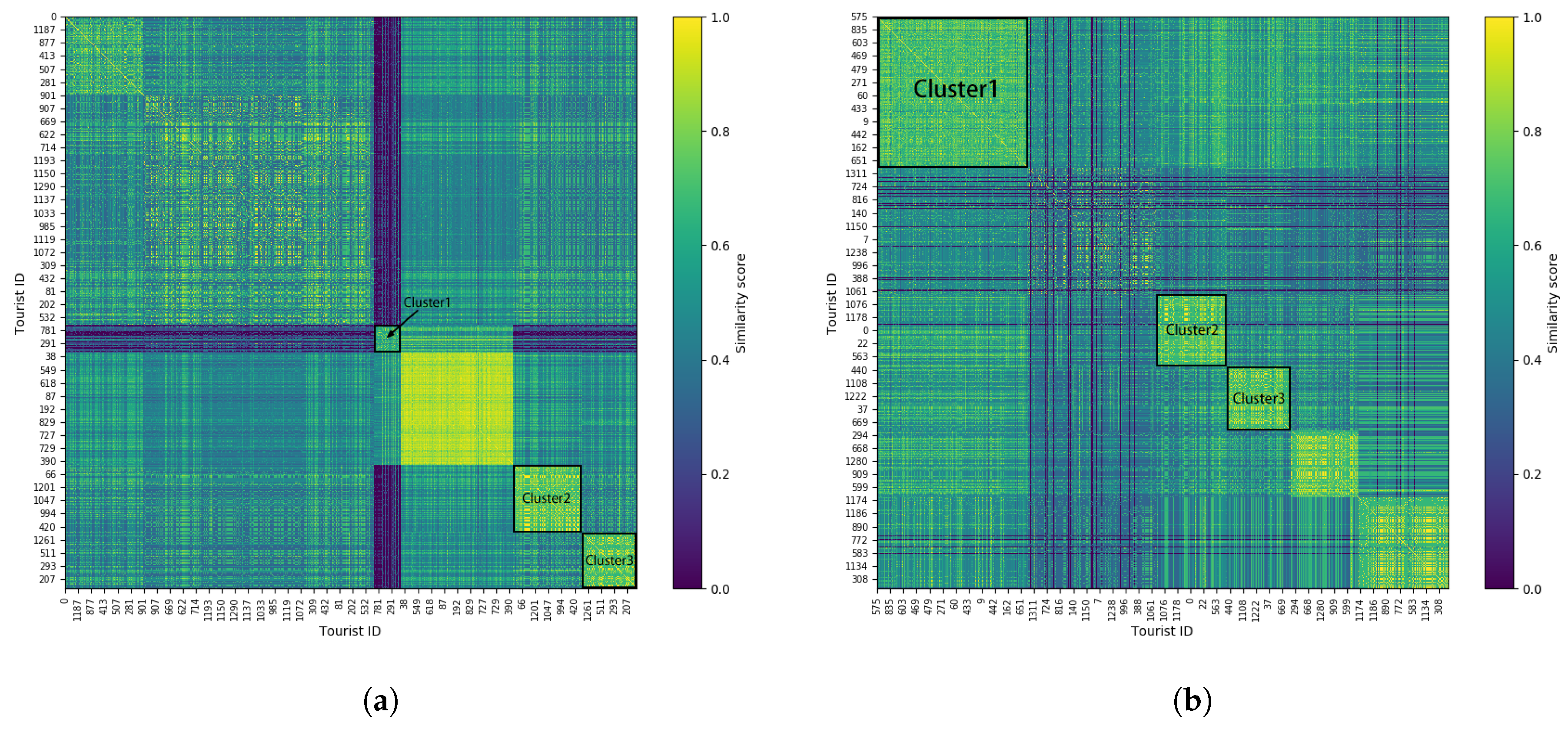
Based on the travel motif-based clustering framework introduced previously in Section 2.3, the similarity scores between each pair of 1312 users that have travel trajectories with at least two nodes are measured. Since topological, temporal and semantic travel motifs are categorized into λ = 5 , γ = 13 and δ = 13 respectively, each tourist is represented by a 31-dimension vector. The resultant similarity matrices are illustrated in Figure 6a,b, after performing hierarchical clustering method. Note that in this research, hierarchical clustering is implemented by using Euclidean distance as the metric for calculating each pair of vectors and the average-link clustering criteria as a function of the pairwise distances of vectors in two clusters [33]. In the similarity matrix, each row represents a similarity vector with 1312 elements, which are the similarity scores with himself/herself and other users. All users’ vectors constitute the similarity matrix (1312 rows × 1312 columns).
According to Equation (19), the similarity matrix is symmetric, and each row (column) stands for a user’s similarity vector. Yellow color denotes high similarity, while dark blue denotes low similarity. For the sake of readability, user ID labels are annotated by skipping every 30 users. There are several noticeable clusters, and for illustration, 12 users in six distinct clusters derived from discrete and consecutive sequences are randomly selected as samples to analyze and understand the underlying travel behavior patterns hereafter.
For discrete sequences as shown in Figure 6a:
  • Cluster 1 denotes tourists who relate to uncommon topological travel motifs, i.e., “cycle”, “downlinked mutual dyad”, “central linked dyad” and “uplinked dyad”. Take Tourist 781 and 291 as examples. Tourist 781 traveled to “Empire State Building → Ground Zero → Brooklyn Bridge → Empire State Building” in a “circle” pattern. Tourist 291 has two trips to New York. The first trip “Time Square → Greenwich Village → Time Square” pertains to the “mutual dyad” topological pattern, and the second trip “Grand Central Terminal → Time Square” is a “chain”. The same characteristic of their trips is that “mutual dyad” exists in both of them.
  • Unlike Cluster 1, Cluster 2 represents tourists following the common “chain” topological travel motif. Furthermore, this group of tourists is more interested in “business” than “cultural” and has the least interest in “natural” attractions. For instance, Tourists 66 and 1201 visited “business → business → cultural → cultural” and “business → cultural”, respectively. They both take “Empire State Building” (a “business” attraction) as the first choice and “cultural” attractions as later targets. Besides, they did not travel to “natural” attractions.
  • Tourists in Cluster 3 follow the “chain” topological pattern like those in Cluster 2, but they have a preference for “cultural” rather than “business”. For example, Tourists 1261 and 207 traveled to “Greenwich Village → Rockefeller Center” and “Time Square → Rockefeller Center → Central Park → Central Park Zoo”, respectively. They both firstly visited a “cultural” attraction followed by a “business” place (i.e., “Rockefeller Center”).
For consecutive sequences as shown in Figure 6b:
  • Cluster 1 contains tourists who like to stay in the first and second place for a similar duration. Taking Tourists 835 and 469 as examples, following “chain” topological travel motifs with three and eight places respectively, they both spent little time in the first and second places and more time in their remaining visitations.
  • Cluster 2 represents tourists who prefer to visit “natural” attractions firstly. Taking Tourists 563 and 0 as examples, Tourist 563 visited “Central Park → Brooklyn Bridge → Rockefeller Center”, and Tourist 0 visited “Central Park → Ground Zero → Greenwich Village → Empire State Building”. They both take the “natural” attraction “Central Park” as the first target.
  • Cluster 3 stands for a group of tourists who are more interested in both “cultural” and “natural” than “business”. For example, Tourist 37 follows a semantic travel motif “cultural → cultural → natural → natural → cultural → natural → cultural”, without “business” attractions visited. Tourist 868 followed the semantic travel motif “natural → cultural → business → natural”, traveling to a “business” attraction after “cultural” and “natural” attractions.
In conclusion, tourists with different travel preferences are separate from each other, and those with similar interests are clustered together, which shows the capability of the proposed framework for unveiling diverse tourists’ travel behavior patterns, which is vital for practical personal travel recommendation.

4. Discussion

As indicated by formal definitions and previous empirical results in Section 2 and Section 3, Schneider’s topological motif, discrete topological motif and consecutive topological motif, as well as their corresponding temporal and semantic motifs, are different from each other. From a theoretical perspective, discrete motif unveil the “relative” priority for visiting different tourism attractions. Put simply, within a set of candidate landmarks, the discrete motif can assist tourists to determine to visit which first based on the collective intelligence of others. However, it cannot provide recommendation to tourists for deciding which landmark to visit immediately next to his/her current landmark. Hence, we developed a consecutive motif to address this “exact” priority problem. Compared with the discrete motif, the consecutive motif produces a continuous travel path between candidate landmarks. It thus enables us to recommend a candidate “next” destination for tourists. Additionally, as previously mentioned, Schneider’s motifs can be regarded as a subset of consecutive motifs.
It is also noteworthy that several improvements can be made in our future works. Among them, the three most important points are listed as follows. (1) Including textual information: This study only utilizes the location and captured time of photos to derive tourists’ mobility patterns. However, text data like tags and titles contain much information about trips. Therefore, a future direction can take text data into consideration for detecting additional contexts of trips, which are of great importance to enrich the knowledge of tourists’ behaviors. (2) Finer classification of attractions: This work classifies landmarks simply into three categories, which are very rough. A finer classification of landmarks will distinguish tourists better. For instance, two tourists sharing an interest in museums are more similar than others who like to visit other cultural places, such as churches. Therefore, constructing a semantic hierarchy with different granularities can be another direction of improvement to this research work. (3) Considering demographics of tourists: People from different countries usually have different preferences in many things, such as eating habits, styles of clothes and genres of art, just to name a few. Similarly, tourists with diverse cultural backgrounds are expected to behave differently in their tourism travel patterns. In this sense, by including the demographic background of tourists, we will be able to deepen our understanding of tourist behavior patterns.

5. Conclusions

Serving as the prerequisite to travel recommender systems, detecting and visualizing tourists’ frequent travel patterns is of great importance for effective travel itinerary planning. With the assistance of geo-tagged photos from Flickr, this research explored tourist behavior patterns based on a novel motif-based clustering framework. Enlightened by previous work on human mobility and network motifs, we extended the concept of travel motifs from topological spaces, to temporal spaces and to semantic spaces and unveiled tourist behavior patterns from different perspectives. In summary, the topological travel motif reveals typical travel patterns (e.g., popular/frequent travel sequence) of tourists between a given number of tourism attractions; the temporal travel motif indicates the time budgets (e.g., the duration of stay) of tourists spent based on the order of visited attractions; and the semantic travel motif differentiates the sightseeing tastes of tourists among different types (e.g., natural, cultural, business, and so on) of tourism attractions.
Our proposed analytic framework will enhance the state of the art tourism studies and recommendation systems in three directions. First, typical topological travel motifs enable tourists to determine the number of attractions to visit and the optimal route. Second, typical temporal travel motifs further enable tourists to determine the visitation duration based on the order of attractions. Third, typical semantic travel motifs enable tourists to determine which type of attraction to visit with high priority. More importantly, this kind of recommendation is different from the state of the art tourism studies and recommendation systems in that it requires no frequent travel sequence covering exactly the same attractions and travel routes. It therefore can remarkably enhance the flexibility of existing tourism recommendation systems to meet more general sightseeing preferences.
Additionally, empirical results derived from Manhattan Island, New York, indicate that tourists tend to travel in space and time with a limited collection of typical topological, temporal and semantic characteristics. These findings confirm that the proposed analytical framework for quantifying user similarity, which consists of representing travel trajectories by motifs and then calculating the closeness of transformed trajectories, provides a promising technique for understanding tourist behavior patterns with explicit spatial, temporal and semantic characteristics. It will enable tourists who want to visit New York to make travel arrangements in a more efficient manner. Last, but not least, concepts and methods introduced by this research can be applied to the study of other mobility datasets and cities and contribute to the development of tourism business in a general sense.

Acknowledgments

The authors gratefully acknowledge the suggestions from the anonymous reviewers. This research is partial funded by the National Natural Science Foundation of China (No. 41601484), the National Key Research and Development Project (No. 2017YFB0503604), the China Postdoctoral Science Foundation (No. 2015M580666), the Open Research Fund of State Key Laboratory of Information Engineering in Surveying, Mapping and Remote Sensing (No. 15S01) and the Fundamental Research Funds of the Central Universities (No. 2042016kf0055).

Author Contributions

C.K. and L.Y. conceived of and designed the experiments. L.Y. performed the experiments. C.K. and L.Y. analyzed the data. L.Y. contributed reagents/materials/analysis tools. C.K., L.Y., Y.L. and L.W. wrote the paper.

Conflicts of Interest

The authors declare no conflict of interest. The founding sponsors had no role in the design of the study; in the collection, analyses, or interpretation of data; in the writing of the manuscript, and in the decision to publish the results.

References

  1. Zheng, Y.; Zhou, X. Computing with Spatial Trajectories, 1st ed.; Springer Science & Business Media: Berlin/Heidelberg, Germany, 2011. [Google Scholar]
  2. Zheng, Y.; Zhang, L.; Xie, X.; Ma, W.Y. Mining Interesting Locations and Travel Sequences from GPS Trajectories. In Proceedings of the 18th International Conference on World Wide Web (WWW ’09), Madrid, Spain, 20–24 April 2009; ACM: New York, NY, USA, 2009; pp. 791–800. [Google Scholar]
  3. Zheng, Y.; Zhang, L.; Ma, Z.; Xie, X.; Ma, W.Y. Recommending Friends and Locations Based on Individual Location History. ACM Trans. Web 2011, 5, 1–44. [Google Scholar] [CrossRef]
  4. Lew, A.A.; McKercher, B. Trip Destinations, Gateways and Itineraries: The Example of Hong Kong. Tour. Manag. 2002, 23, 609–621. [Google Scholar] [CrossRef]
  5. Mckercher, B.; Lau, G. Movement Patterns of Tourists within a Destination. Tour. Geogr. 2008, 10, 355–374. [Google Scholar] [CrossRef]
  6. Wood, S.A.; Guerry, A.D.; Silver, J.M.; Lacayo, M. Using Social Media to Quantify Nature-Based Tourism and Recreation. Sci. Rep. 2013, 3, srep02976. [Google Scholar] [CrossRef] [PubMed]
  7. Kavitha, S.; Jobi, V.; Rajeswari, S. Tourism Recommendation Using Social Media Profiles. In Artificial Intelligence and Evolutionary Computations in Engineering Systems; Springer: Singapore, 2017; pp. 243–253. [Google Scholar]
  8. Liu, Y.; Sui, Z.; Kang, C.; Gao, Y. Uncovering Patterns of Inter-Urban Trip and Spatial Interaction from Social Media Check-In Data. PLoS ONE 2014, 9, e86026. [Google Scholar] [CrossRef] [PubMed]
  9. Yuan, Y.; Medel, M. Characterizing International Travel Behavior from Geotagged Photos: A Case Study of Flickr. PLoS ONE 2016, 11, e0154885. [Google Scholar] [CrossRef] [PubMed]
  10. Popescu, A.; Grefenstette, G.; Moëllic, P.A. Mining tourist information from user-supplied collections. In Proceedings of the 18th ACM Conference on Information and Knowledge Management, Hong Kong, China, 2–6 November 2009; ACM: New York, NY, USA, 2009; pp. 1713–1716. [Google Scholar]
  11. Kennedy, L.; Naaman, M.; Ahern, S.; Nair, R.; Rattenbury, T. How Flickr Helps Us Make Sense of the World: Context and Content in Community-Contributed Media Collections. In Proceedings of the 15th ACM international conference on Multimedia, Augsburg, Germany, 23–28 September 2007; ACM: New York, NY, USA, 2007; pp. 631–640. [Google Scholar]
  12. Zeng, Z.; Zhang, R.; Liu, X.; Guo, X.; Sun, H. Generating Tourism Path from Trajectories and Geo-Photos. Proceedings of the 13th International Conference on Web Information Systems Engineering, Paphos, Cyprus, 28–30 November 2012; Wang, X.S., Cruz, I., Delis, A., Huang, G., Eds.; Springer: Berlin/Heidelberg, German, 2012; pp. 199–212. [Google Scholar]
  13. Paldino, S.; Bojic, I.; Sobolevsky, S.; Ratti, C.; González, M.C. Urban Magnetism through the Lens of Geo-Tagged Photography. EPJ Data Sci. 2015, 4, 5. [Google Scholar] [CrossRef]
  14. Arase, Y.; Xie, X.; Hara, T.; Nishio, S. Mining People’s Trips from Large Scale Geo-Tagged Photos; ACM Multimedia: Mountain View, CA, USA, 2010; pp. 133–142. [Google Scholar]
  15. Lu, X.; Wang, C.; Yang, J.M.; Pang, Y.; Zhang, L. Photo2trip: Generating Travel Routes from Geo-Tagged Photos for Trip Planning. In Proceedings of the 18th ACM International Conference on Multimedia, Firenze, Italy, 25–29 October 2010; ACM: New York, NY, USA, 2010; pp. 143–152. [Google Scholar]
  16. Zheng, Y.T.; Zha, Z.J.; Chua, T.S. Mining Travel Patterns from Geotagged Photos. ACM Trans. Intell. Syst. Technol. 2012, 3, 1–18. [Google Scholar] [CrossRef]
  17. Sun, Y.; Fan, H.; Bakillah, M.; Zipf, A. Road-Based Travel Recommendation Using Geo-Tagged Images. Comput. Environ. Urban Syst. 2015, 53, 110–122. [Google Scholar] [CrossRef]
  18. Vu, H.Q.; Li, G.; Law, R.; Ye, B.H. Exploring the Travel Behaviors of Inbound Tourists to Hong Kong Using Geotagged Photos. Tour. Manag. 2015, 46, 222–232. [Google Scholar] [CrossRef]
  19. Becker, M.; Singer, P.; Lemmerich, F.; Hotho, A.; Helic, D.; Strohmaier, M. Photowalking the City: Comparing Hypotheses About Urban Photo Trails on Flickr; SocInfo: Oxford, UK, 2015; pp. 227–244. [Google Scholar]
  20. Clements, M.; Serdyukov, P.; De Vries, A.P.; Reinders, M.J. Using Flickr Geotags to Predict User Travel Behaviour. In Proceedings of the 33rd International ACM SIGIR Conference on Research and Development in Information Retrieval, Geneva, Switzerland, 19–23 July 2010; ACM: New York, NY, USA, 2010; pp. 851–852. [Google Scholar]
  21. Majid, A.; Chen, L.; Chen, G.; Mirza, H.T.; Hussain, I.; Woodward, J. A Context-Aware Personalized Travel Recommendation System Based on Geotagged Social Media Data Mining. Int. J. Geogr. Inf. Sci. 2013, 27, 662–684. [Google Scholar] [CrossRef]
  22. Barchiesi, D.; Preis, T.; Bishop, S.; Moat, H.S. Modelling Human Mobility Patterns Using Photographic Data Shared Online. R. Soc. Open Sci. 2015, 2, 150046. [Google Scholar] [CrossRef] [PubMed]
  23. Beiró, M.G.; Panisson, A.; Tizzoni, M.; Cattuto, C. Predicting Human Mobility Through the Assimilation of Social Media Traces into Mobility Models. EPJ Data Sci. 2016, 5, 30. [Google Scholar] [CrossRef]
  24. Milo, R.; Shen-Orr, S.; Itzkovitz, S.; Kashtan, N.; Chklovskii, D.; Alon, U. Network Motifs: Simple Building Blocks of Complex Networks. Science 2002, 298, 824–827. [Google Scholar] [CrossRef] [PubMed]
  25. Jackson, M.O. Social and Economic Networks; Princeton University Press: Princeton, NJ, USA, 2008. [Google Scholar]
  26. Kovanen, L.; Karsai, M.; Kaski, K.; Kertész, J.; Saramäki, J. Temporal Motifs in Time-Dependent Networks. J. Stat. Mech. Theory Exp. 2011, 2011, P11005. [Google Scholar] [CrossRef]
  27. Schneider, C.M.; Belik, V.; Couronné, T.; Smoreda, Z.; González, M.C. Unravelling Daily Human Mobility Motifs. J. R. Soc. Interface 2013, 10, 20130246. [Google Scholar] [CrossRef] [PubMed]
  28. Kurashima, T.; Iwata, T.; Irie, G.; Fujimura, K. Travel Route Recommendation Using Geotags in Photo Sharing Sites. In Proceedings of the 19th ACM International Conference on Information and Knowledge Management, Toronto, ON, Canada, 26–30 October 2010; ACM: New York, NY, USA, 2010; pp. 579–588. [Google Scholar]
  29. Kurashima, T.; Iwata, T.; Irie, G.; Fujimura, K. Travel Route Recommendation Using Geotagged Photos. Knowl. Inf. Syst. 2013, 37, 37–60. [Google Scholar] [CrossRef]
  30. Shao, H.; Zhang, Y.; Li, W. Extraction and Analysis of City’s Tourism Districts Based on Social Media Data. Comput. Environ. Urban Syst. 2017, 65, 66–78. [Google Scholar] [CrossRef]
  31. Shi, Y.; Serdyukov, P.; Hanjalic, A.; Larson, M. Personalized Landmark Recommendation Based on Geotags from Photo Sharing Sites. In Proceedings of the 5th International AAAI Conference on Weblogs and Social Media, Barcelona, Spain, 17–21 July 2011; Volume 11, pp. 622–625. [Google Scholar]
  32. Thomee, B.; Shamma, D.A.; Friedland, G.; Elizalde, B.; Ni, K.; Poland, D.; Borth, D.; Li, L.J. YFCC100M: The New Data in Multimedia Research. Commun. ACM 2016, 59, 64–73. [Google Scholar] [CrossRef]
  33. Jain, A.K.; Murty, M.N.; Flynn, P.J. Data Clustering: A Review. ACM Comput. Surv. 1999, 31, 264–323. [Google Scholar] [CrossRef]
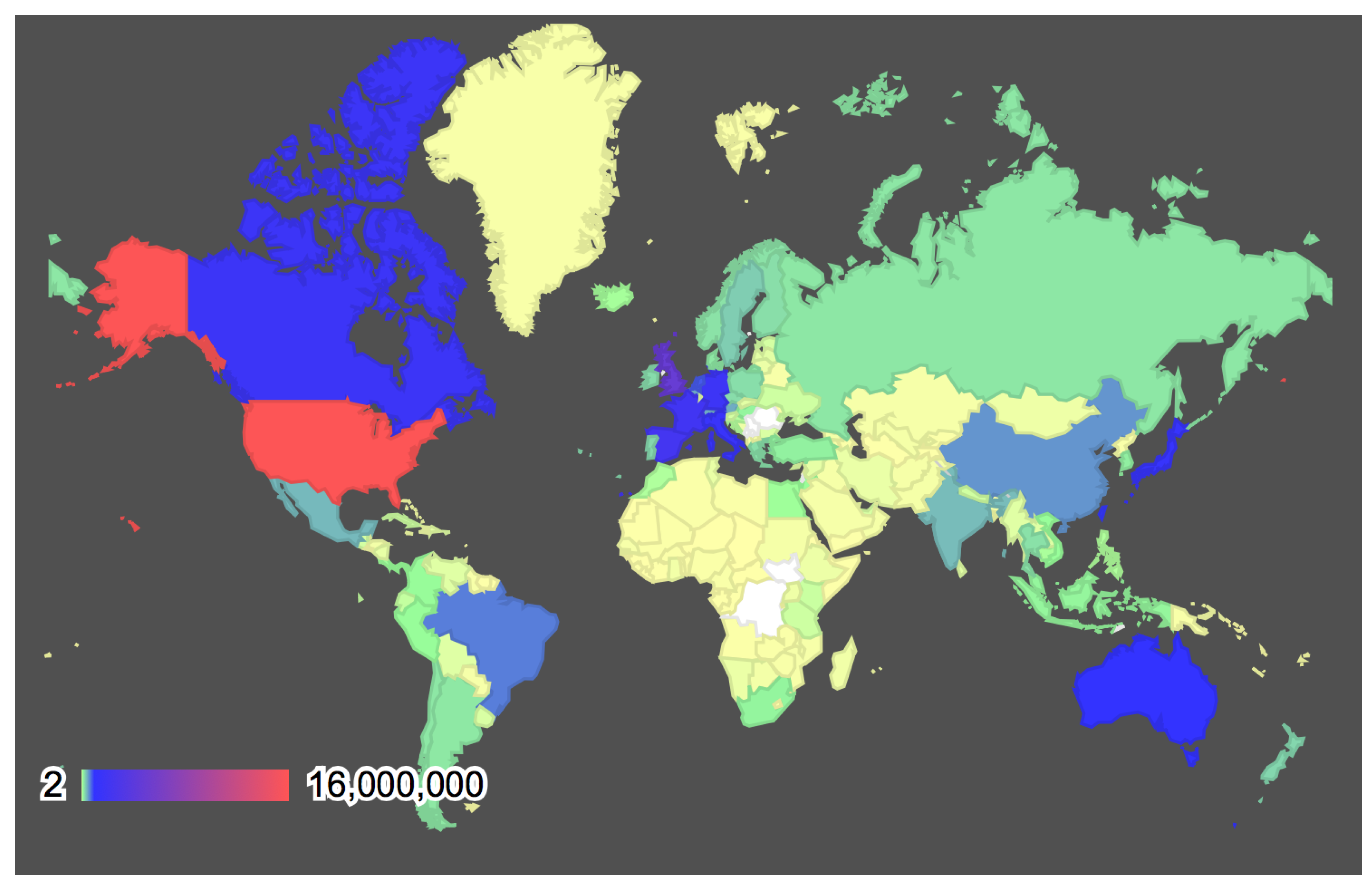
Figure 1. One million photo sample of the 48 million geo-tagged photos from the Yahoo Flickr Creative Commons 100M (YFCC100m) dataset plotted around the globe (image source: The Competence Center Multimedia Analysis and Data Mining (MADM) at the DFKI).
Ijgi 06 00345 g001
Figure 2. (a) Top 30 popular landmarks and (b) an example travel path in Manhattan.
Ijgi 06 00345 g002
Figure 3. Dendrogram of topological travel motifs based on (a) discrete sequence and (b) consecutive sequence. Note that N denotes the number of attractions within the identified motif; the value above each motif indicates the threshold ϵ m % for detecting it as a significant motif; and the “double-linked mutual dyad” motif is excluded for analysis in that its corresponding threshold is lower than 0.05 .
Ijgi 06 00345 g003
Figure 4. Statistical characteristics of temporal travel motifs based on (a) discrete sequence and (b) consecutive sequence.
Ijgi 06 00345 g004
Figure 5. Statistical characteristics of semantic travel motifs based on (a) discrete sequence and (b) consecutive sequence.
Ijgi 06 00345 g005
Figure 6. Travel behavior patterns of distinct tourist groups in terms of (a) discrete sequence and (b) consecutive sequence based motifs. Note that each value in the matrix indicates the similarity between a pair of users based on their topological, temporal and semantic travel motifs.
Ijgi 06 00345 g006