Abstract
The relationship between vegetation, transportation networks, and crime has been under debate. Vegetation has been positively correlated with fear of crime; however, the actual correlation between vegetation and occurrences of crime is uncertain. Transportation networks have also been connected with crime occurrence but their impact on crime tends to vary over different circumstances. By conducting spatial analyses, this study explores the associations between crime and vegetation as well as transportation networks in Kitchener-Waterloo. Further, geographically weighted regression modeling and a dummy urban variable representing the urban center/other urban areas were employed to explore the associations across an urban central-peripheral gradient. Associations were analyzed for crimes against persons and crimes against property for four specific crime types (assaults, vehicle theft, sex offences, and drugs). Results suggest that vegetation has a reverse association with crimes against persons and crimes against property while transportation networks have a positive relationship with these two types of crime. Additionally, vegetation can be a deterrent to vehicle theft crime and drugs, while transportation networks can be a facilitator of drug-related crimes. Besides, these two associations appear stronger in the urban center compared to the urban periphery.
1. Introduction
Crime, known as a perennial, widespread phenomenon, can be classified into two categories, crimes against persons and crimes against property [1]. Crime is a prevalent phenomenon in all societies, accompanied by many costs and, therefore, is of wide concern to residents, police, planners and decision makers. In Canada, there were 5190 incidents per 100,000 people according to Boyce et al. [2], which means that one out of 20 people may be a potential offender.
The cost of crime has always had negative influences on the society and the analysis of crime has consistently been considered as a challenge because crime could be influenced by a large number of factors while their influences may vary in different cities. The research of crime ranges from ecological and psychological to geographical and spatial approaches. These theories of crime based on different approaches can date back to the early nineteenth century [3].
There are three essential elements usually being considered for research on the geography of crime: place, distance, and direction [4]. The place-based theory considers the distribution of crime as the intersection of victims and offenders [1,5]. When time and space are appropriate, motivated perpetrators would commit crimes against suitable targets.
More modern work on crime employing a spatial perspective basically builds on two theories: social disorganization theory and routine activity theory. However, even though both theories can support the explanation of the geography of crime, social disorganization theory tends to be the more well-researched one. According to the routine activity theory, built features and routine activities are two factors influencing crime [5]. Land use can be concerned with specific features as well as unique attractiveness, such as vegetation and transportation networks.
Both vegetation and crime prevention should be considered for urban planning. However, little research has been done to discover the interconnection between vegetation and crime occurrence. Vegetation could be considered as one important factor influencing people’s behaviors while the actual influences remain ambiguous. The correlation between dense vegetation and a higher potential for crime has been well known as vegetation provides the offender concealment [6] and was also positively associated with increased fear of crime [7]. Nevertheless, even though vegetation appears to conceal offenders, more modern research has found the effects of vegetation on crime tend to be mixed and even provide deterrence [8,9,10,11,12]. Kuo and Sullivan [8] suggested that crime appeared to be deterred by high-canopy trees as well as grass. Encouraging use of open space, which has mental restorative effects, appears to control crime.
However, this debate continues, and little research has taken into account the spatial effects in terms of the relationship between crime and vegetation. Moreover, no research has explored this spatial relationship within Canada. Since crime can be considered as a location-based phenomenon, the distribution and situation of crimes may vary depending on the cities’ characteristics. The relationships which exist in other cities and countries cannot be simply referred to in order to explain the situation in Canada. Even though different types of vegetation tend to have various effects on crime, this study considers all green space as vegetation.
There is also debate surrounding the relationship between transportation networks and crime. The first theory linking crime to street use was found by Jacobs [13] and was based on inference. She believed that people on the street could provide informal surveillance, which was known as “the eyes on the street”. As a consequence, she inferred that people would suffer more crimes in areas with few witnesses. However, other researchers have found a positive relationship between crime and high accessibility of road network [14,15,16]. Nevertheless, these studies either used linear models regardless of spatial patterns or employed qualitative methods to provide some suggestions. Even though most researchers realized the spatial association issues during their research, they appeared to consider spatial issues as a nuisance.
Urban characteristics have also been associated with crime. In 1999, Rephann [17] demonstrated that higher crime rates usually emerged in urbanized metropolitan areas in contrast to rural areas. Boggs [18] concluded that the highest crime rates were likely to appear in Central Business Districts (CBDs) within urban areas. However, there is no research that studies the potential different impacts of vegetation and transportation networks on crime at urban central-peripheral gradient. The only study we could find that considered urban-rural gradient for the spatial relationship between crime and vegetation was conducted by Troy et al. [10].
This study investigates the validity of the relationship between crime and variables rooted in routine activity theory, to see whether their relationships can extend beyond specific circumstances, especially for the medium-size city. Secondly, this study addresses the gap in published studies examining the spatial relationship between crime, vegetation, and transportation networks in Canada. Thirdly, the spatial statistical technique is employed in this study instead of the classical statistical techniques in most previous literature. Fourthly, crimes against persons and crimes against property are examined separately with four specific types of crime (assault, sex offenses, drugs, and vehicle theft) tested. Fifthly, the smallest standard geographic unit dissemination area is adopted in contrast to census tracts found in previous literature [11,19], and may provide another insight to illuminate this debate. Finally, the urban central-peripheral gradient is considered to explore the possible spatial non-stationarity existing for the relationship between vegetation, transportation networks, and crime.
We hypothesize that higher vegetation density is related to lower crime density, while higher transportation network density increases crime density. Additionally, vegetation and transportation networks may have a more significant influence on crime in the urban center. We test this hypothesis by conducting spatial regression analyses and inspecting the relationship between crime, vegetation, and transportation networks statistically at the macro-size level. Furthermore, other social-economic or social-demographic variables, which have been known with impacts on crime, were controlled in this study.
2. Literature Review
2.1. Crime Theories Supporting the Spatial Analysis
There are two theories supporting the spatial analysis of criminology: social disorganization theory and routine activity theory [19]. Social disorganization theory refers to those social characteristics related to criminal events, including five factors: demographic, economic, social, family disruption, and urbanization [19,20,21,22,23,24,25]. Because of these factors varying among different neighborhoods, criminal events tend to occur spatially-based. Therefore, social disorganization theory can be considered as an indicator of the incidents of criminal events. However, criminal events may still happen without satisfying these social disorganization factors.
The other theory, routine activity theory, guides the inspection of vegetation and transportation networks in this study. This theory, basically rooted in place theory, emphasizes the combination of offenders, targets, and the absence of guardianship [5,19]. Routine activity theory was first founded by Cohen and Felson [26], who emphasized the importance of the combination of suitable targets and lack of crime suppressors. Place, as one type of medium, providing a direct platform for the connection between people, can influence crime in two ways. One is related to the built features of places, while the other is associated with the routine activities happening in different places [5]. These two ways actually correspond to two causes for criminal events: suitable targets and the absence of guardianship. Guarded or gated communities have strong guardianship, and hence, can be considered defensible space. However, high-rise housing may be believed to be a facility lacking effective monitoring activities because tenants live vertically and public space for residents is limited [27]. Another way for places to affect criminal events are the routine activities happening there. Cohen and Felson [26] argued that the dispersion of activities away from households tends to provide more opportunities for offenders to commit crimes and, hence, boost crime rates. Routine activity theory provides strong explanations in terms of the spatial variety of crimes and the theoretical connection between crimes and places. High rates of crime tend to occur at places sharing some similar facilities or activities, while others do not.
These two theories of crime have also been integrated to understand the geography of crime. Johnstone [28] found that both family and community status could affect aggressive offences. In the study of Smith et al. [29], the number of single-family households, which can be considered a specific land use, accompanied by social characteristics, is related to crime. Single-parent families would be thought as a social demographic factor, and may relate to the concept of guardianship in the neighborhood. This single-parent family factor can be seen as an indicator in routine activity theory [30].
2.2. Crime and Vegetation
Crimes can be correlated with specific geographic features [31]. Vegetation, as a special aspect of the physical environment, can be considered as one factor guided by routine activity theory. There are two basic schools of thought regarding the link between vegetation and crime. The first refers to the tradition to removing vegetation because it conceals and facilitates criminal acts [7,32]. In one study, interviews conducted within 97 Detroit residences demonstrated that densely wooded areas appeared to be more associated with the fear of dangerous situations [33]. In another study, college students rated the attractiveness and the security perception for 180 parking lots and the results presented were that unmaintained, natural vegetation tended to increase people’s fear of crime [34]. Based on extensive on-site interviews, Michael et al. [35] explored how physical features in parks could be used by offenders and found them positively associated with auto burglaries. A variety of evidence has linked the presence of dense vegetation to fear of crime [8]. The reasons why individuals felt more vulnerable in densely forested areas may be explained by the fact that vegetation blocks views [7,34] and provides space for criminals to hide [6].
Common themes of these studies highlighted people’s ability to observe his or her surroundings. If a resident cannot see his or her surroundings clearly, it is more likely that he or she will feel more vulnerable to criminal activities. Perpetrators may also choose these places to conceal their behavior. As a consequence, vegetation could provide cover for criminal events and potentially increase the possibility of crime and certainly the induced fear of crime, but it could only be regarded as one of the factors influencing crime occurrence [8]. Few studies supporting this school of thought examined the relationship between vegetation and crime at a large-scale level.
The other school of thought regarding the relationship between crime and vegetation emphasizes that vegetation can be considered a crime deterrent. Recent studies have found that the presence of trees, grass and shrubs might actually deter criminal activities. As mentioned by Kuo and Sullivan [8], vegetation was considered to inhibit crime through two mechanisms: by providing more surveillance, and by alleviating some of the psychological precursors to violent behavior. As one significant part of urban design, treed outdoor space tends to be widely well-used by youths, adults, and mixed-age groups compared to treeless space. Because of this attractiveness, more eyes on the street were introduced [8]. This finding has also been demonstrated by Donovan and Prestemon [12]. In Donovan and Prestemon’s study [12], the presence of street trees and large trees appeared to suppress criminal events, while smaller trees still remained a positive association with crime. In addition, Kuo [36] suggested that green outdoor space was linked with a stronger social interaction and hence crime might be decreased. Well-maintained vegetation might indicate that an intruder might be easily noticed [8,37]. Another explanation why well-maintained vegetation can reduce crime is referred to in the “Broken Window” theory [38] which states the “authority” and signifying that this community is under supervision by its residents. Vegetation also provides psychological benefits. Since one of the costs of mental fatigue may be an enhanced propensity for potential violence [39], recovery from mental fatigue would definitely help reduce crime occurrence. More modern research has tried to explore the presence of vegetation and crime by using a quantitative method. A strong inverse association between crime rates and tree canopy cover has been suggested, especially for public land [10]. Additionally, Wolfe and Mennis [11] demonstrated that vegetation abundance is associated with lower crime rates for assault, robbery, and burglary in Philadelphia.
Even though researchers have realized that criminal events tend to vary between different places and may present as clusters, most of them favor classical statistical analyses [19] and qualitative methods [10]. Both methods have their limitations. Qualitative methods cannot inspect crimes in a large scale area while classical statistical analyses cannot assess neighborhood effects. For those studies inspecting the association between crime and vegetation, there were only two that have employed spatial analysis [10,11]. As a consequence, this association should be further explored by using spatial regression models that may provide better assessment of spatial patterns regarding the presence of vegetation and crime.
2.3. Crime and Transportation Networks
Connecting street design to crime has been studied for a long time. By clearing slums, Tobias [40] noted that new streets could be built as part of urban planning. Jacobs [13], as the first contemporary urban planner intending to outline the theory to support the relationship between crime and the street, argued that citizens on the street could provide informal surveillance and, hence, became the “eyes of the street”. Crimes in public could be reduced based on her theory by creating a moderate street network. Newman [27] expounded on this idea by introducing the term “territorial subdivision”. He stated that strangers could be better recognized as invaders because the territorial subdivision of streets increased. As a consequence, street networks could contribute to the reduction of crime.
Brantingham and Brantingham [41] noted that people who committed crimes against property usually chose easily knowable spaces, where they could easily find escape routes. However, the complexity of road networks may make this more difficult. The study of crime from Bevis and Nutter [14] revealed the possibility that burglary rates were reduced because the complexity of road networks were increased in criminally attractive areas. They also contended that lower accessibility meant fewer burglaries and that rising crime rates were significantly correlated with the increase of street accessibility, based on their research in Minneapolis, MN, USA. They found that the highest burglary rates happened at houses built on corners [42] while dead-end streets suffered the lowest burglary rates [14].
More modern research suggested that dense road networks would create more opportunities for offenders and targets to meet as well as attracting strangers. Brantingham and Brantingham [43] highlighted the role of paths in determining people’s routine activities. They argued that property offenders liked to commit offences in known spaces. The study of Beavon et al. [15] demonstrated that higher accessibility of road networks and higher levels of traffic flow would contribute to more crimes against property. Jarrell and Howsen [44] argued that highways can enhance the number of transient populations. Therefore, the number of strangers had a positive effect on the occurrence of burglary, larceny, and robbery. Rephann [17] also contended that highway construction can exacerbate crime rates in rural regions by increasing population mobility. However, all of these studies were based on linear models regardless of the spatial correlation. Groff et al. [16] also explored the relationship between crime and street from the micro-level. Their research did not demonstrate a quantitative spatial association. They concluded that traffic levels can be employed as an indicator representing the number of people within the block and hence tends to increase the opportunity for the convergence of offenders and targets.
2.4. Crime in Urban Areas
Urbanization has long been related to the convergence of different types of crime. Rephann [17] noted that urbanization had a strong effect on crime by examining the degree of urbanization as a dummy variable. More recent directional analyses of crime pointed out that offenders prefer urban areas [45]. Even within urban areas, different districts, which might be affected by social factors or physical environment, such as poverty, economic class, and neighborhoods, etc., tend to experience different crime rates. According to Boggs [18], by summarizing previous studies of crime in intra-city distribution, central business districts appear to be connected with the highest crime rates. However, Jacobs [13] inferred that non-residential usage of one district can provide more surveillance and hence deter crime occurrences. Pyle et al. [46] noted that the city center was known for the heaviest concentration of violent crimes and even areas attributed to urban renewal programs presented the highest reporting of crimes. Additionally, Frank et al. [4] emphasized the existence of the convergence of offenders in the downtown area in Prince George.
The spatially non-stationarity appears to have an influence on crime distribution. However, the question in terms of whether this spatially non-stationarity exists for the relationship between vegetation, transportation networks, and crime appears to be forgotten by scholars. The only study inspecting the relationship between crime and vegetation at urban-rural gradient was provided by Troy et al. [10]. They employed geographically weighted regression models for all of Baltimore county and found the spatially non-stationarity exists for vegetation. A positive relationship between crime and vegetation was found for some isolated areas, such as areas around harbor facilities, while the vegetation in remaining areas either had a negative association or did not have a statistical association with crime. There was a gap between literature that inspected the spatial relationship between vegetation, transportation networks, and crime at the urban central-peripheral gradient.
3. Crime in the Kitchener-Waterloo Region: Study Area and Data
3.1. Study Area
Kitchener and Waterloo are twin cities located in the south-central area of Ontario, Canada. These two cities are often jointly referred to as “Kitchener-Waterloo” or “KW”, although they have different city governments. Many public services in Kitchener-Waterloo are provided by regional services, such as police and public transit. At the time of the 2011 census, the population of Waterloo was 98,780 while the population of Kitchener was 219,153. The City of Waterloo covers 64.10 square kilometers and the City of Kitchener covers 136.86 square kilometers.
More than half of the study area is dominated by non-forested land cover, known as built-up areas or impervious surfaces. The forested portion of the study area is composed of mixed forest and cropland [47]. Ottawa Street, Highland Road, King Street, and University Avenue, known as arterial roads among this region, provide intercity connections. Highway 85, Highway 7 and Highway 8 are three highways in this region, and are important parts of the city’s transportation system.
This region has a strong knowledge- and service-based economy supported by a large quantity of high-tech companies and three post-secondary institutions. However, crime is a significant issue in this region, influencing people’s daily lives. Both violent crime rates and property crime rates in Waterloo Region were higher than the average crime rates for Ontario from 2010 through 2013 [48]. The total crime rate in Waterloo Region in 2013 was 4366 per 100,000 people compared to only 2941 per 100,000 people in Toronto, the provincial capital of Ontario [49]. Specifically, the violent crime rate per 100,000 people was 847, the property crime rate was 2897, while other criminal code offences numbered 592, and the rate for drug offences was 316.
Figure 1 below presents the distribution of criminal events in Kitchener-Waterloo Region in 2013. The legend presents different levels of crime density, ranging from 0 to 0.0271. The calculation of crime density was based on crime counts and land area, for which crime count was divided by land area in each dissemination area. Regional core areas were places with more convergence between offenders and targets. However, whether spatial clusters contributed to the occurrence of crimes should be examined further.
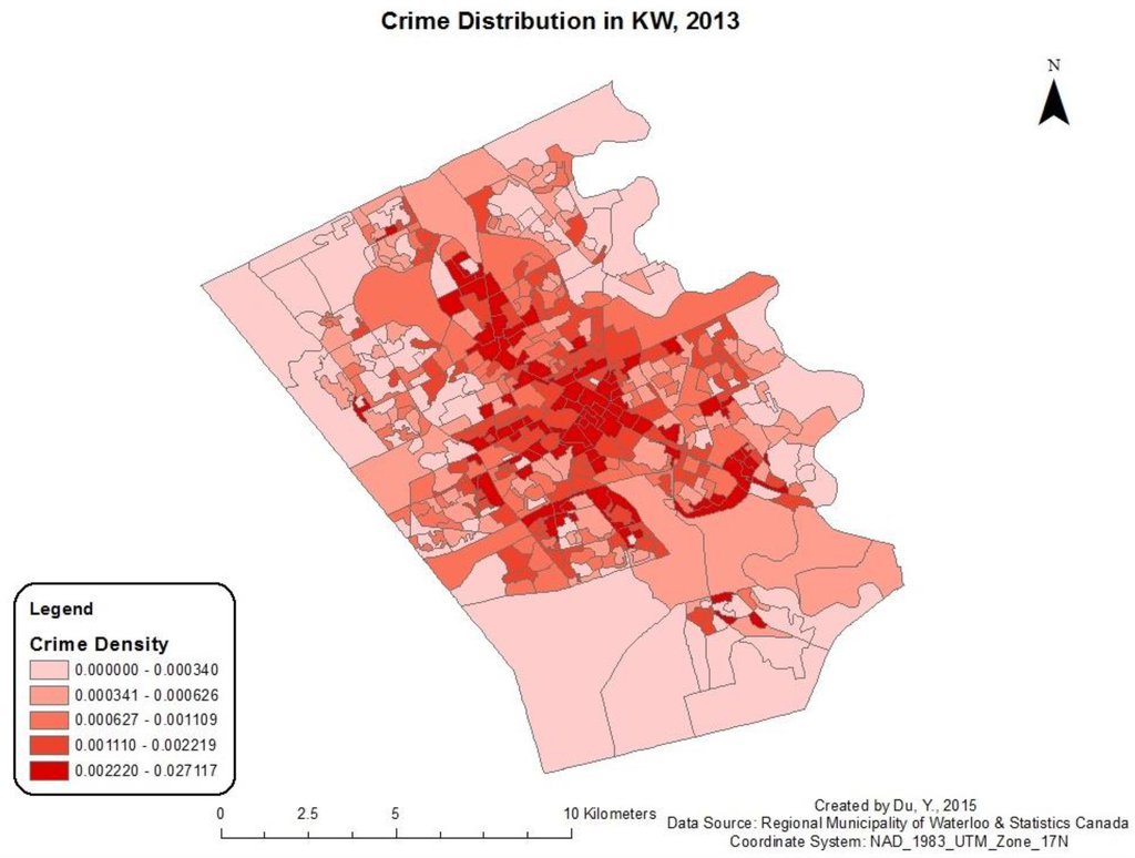
Figure 1.
Crime distribution in the Kitchener-Waterloo region, 2013.
3.2. Crime Data
The crime report was downloaded from the website of the Waterloo Regional Police Services [48]. This report was shared by WRPS as open data and it included all crime call records for the year 2013. This dataset contains each call with detailed information, including date, time, location, first call type, final definition, and coordinates, etc. For each record, a final definition of crime type, as well as coordinates provided, was the most important attribute to obtaining valuable information for this study. These records also covered all types of crimes, such as assault, graffiti, threats and property damage, etc. Because of all of the information provided, each crime point could be geocoded and classified. Each crime record, therefore, was presented as a point after the whole dataset was geocoded.
3.3. Socio-Demographic and Socio-Economic Data
Two datasets, categorized as income and population, were obtained from Statistics Canada’s 2011 census data, distributed by the Geospatial Center at the University of Waterloo. These datasets are the latest datasets provided for socio-demographic and socio-economic information, since the year 2011, the latest census year in Canada. The two datasets were both obtained at dissemination area levels following new rules set up in 2011. The partition of dissemination areas in Canada led by the federal government had changed from 2006 to 2011, but it remained the same from 2011 until 2015. As a consequence, these datasets can be joined easily for further analyses. Additionally, the dissemination area is the smallest standard geographic area in Canada with a population of 400 to 700 people, but the size of each dissemination area varies among urban areas. Densely populated dissemination areas usually have smaller sizes than sparsely populated dissemination areas. Hence, data at the dissemination area level may provide another insight at the “micro” level compared to data at the census tract level.
3.4. Land Use Data
Vegetation data was derived from satellite imagery. One image from Landsat-5 TM was collected on 17 May 2009 at path 18, row 30 and downloaded from the U.S. Geological Survey (USGS). Six bands of 30-m resolution were used for land use classification. The coordinate system used was WGS84 and the projection was UTM Zone 17N. The RADARSAT-2 image employed was one scene of a single look complex (SLC) collected on 19 April 2009 in the ascending direction with fine quad polarization, retrieved from the Canadian Space Agency. Temporal change can affect land cover while dense vegetation can be distinguished in the season selected by this study. The image from the RADARSAT-2 is at 8-m resolution with full polarization (HH, HV, VH, and VV). The Random Forest Classifier (RFC) [50,51] was adopted to generate the classification map by integrating variables generated by Landsat and RADARSAT-2 images with quad polarization. The Random Forest Classifier can be considered a combination of tree classifiers with one pixel classified by choosing the class with the most votes from all tree predictors in the forest [50]. Developed from decision tree classifiers [52], RFC is also nonparametric and can adapt to nonlinear relations, which is more suitable in the urban context [53]. The total number of variables put into the RFC reached 90, which was composed of bands and calculated textures. Additionally, in order to integrate Landsat images with RADARSAT images, the Landsat image was resampled to 8-m resolution and hence the final classification result was encoded as an 8-m resolution image. A total of 500 hundred random sample points were elected in order to examine the accuracy of results. The overall accuracy for the land cover classification reached 86.8% while the average accuracy for vegetation was even higher. The producer’s accuracy for vegetation was 94.5% and the user’s accuracy for vegetation was 92.3%. The high accuracy of vegetation data enhanced the reliability of this study. Also, the resolution of this land use map can distinguish intermediate and large greenspaces so that areas with enough green cover can be taken into account.
Transportation network data were obtained for 2013 from the Geospatial Center at the University of Waterloo and originally provided by the Regional Municipality of Waterloo. All of the road systems within the Kitchener-Waterloo Region were included in this dataset, containing expressways/highways, arterial roads, collectors, local streets, and private streets, etc. Among 9359 segments in this dataset, 8428 of them were public roadways. The length of each segment was also provided as one attribute. This dataset could be further applied to calculate transportation network density.
4. Inspecting the Spatial Issues: Methodology
4.1. Preprocessing
Before running different statistical models, a series of preprocessing steps had to be conducted to obtain those calculable variables, either dependent or independent variables. We sought to acquire various socio-economic and socio-demographic variables associated with crime. Previous studies have shown that poverty has the greatest explanatory power for crime occurrence [54], and single-parent families has been connected with neighborhood, because single-parent families may provide less guardianship and thus can be positively associate with crimes [29,55]. Additionally, population density was examined by Cahill and Mulligan [56] and single-family households were tested by Troy et al. [10]. Three of six explanatory variables selected were based on social disorganization theory, one integrated both social disorganization and routine activity theory, and the remaining two variables were potential impacts rooted in routine activity theory. Poverty density was measured based on each dissemination area, for which the population with income in the bottom decile was divided by the land area of each dissemination area. According to Statistics Canada [57], the low-income line used in Canada fluctuated from 9% to 16% over the past 34 years. As a consequence, the population with income in the bottom decile was chosen as the population in poverty, while its use was still somewhat arbitrary. Population density was also included, as the ratio of the total population to land area within each dissemination area. In addition, single-parent family density was calculated as the ratio of the number of single-parent families to land area within each dissemination area, and one family household density was calculated as the ratio of the number of one family households to land area within each dissemination area.
Instead of using percentage of land area covered by the tree canopy [10] or NDVI [11] to represent vegetation, vegetation density was employed in this study. Vegetation density was derived from the land use/land cover classification map. The classification result had to be transferred to vector data first since the original classification result was raster data. By transferring raster data to vector data, each pixel was transferred to one point, which meant one point represented 8 × 8 m2. The whole pixel had to be classified as one class only, either vegetation, water or impervious area, etc. so that the single tree canopy cannot be distinguished in this study. The vegetation used in this study targeted on a large portion of green space, which can be garden, forest, grassland, or even green farmland being distinguished at the 8 × 8 m2 level. In addition, since each pixel was a square, some pixels may be divided by the boundary of two areas. For this situation, the pixel can only belong to one area based on the location of its centroid point. The vegetation class used here kept the high accuracy for the large proportion green space. By selecting the vegetation class only, vegetation area could be calculated. Then, the ratio of vegetation area to land area within each dissemination area could be used as vegetation density.
Transportation network density was measured as the ratio of the total length of road networks to land area within each dissemination area. The calculation of transportation network density was based on the definition from the World Bank in terms of road density indicators. However, intersect tools had to be applied first since some roadways may traverse several areas while only road segments within one area could be counted for that specific area.
Different crime densities were also calculated separately. Crime density was considered as the variable instead of crime count or crime rate, since the size of spatial units should be considered to represent the severity in different locations. Because each crime record was a point, the total number of crimes could be counted and divided by the land area of each dissemination area in order to obtain the crime density. Crime densities were acquired for different types: crimes against property, crimes against persons, assaults, sex offences, vehicle thefts, and drugs. Crimes against persons used in this study included 9 different offence types: assault, liquor offences, criminal harassment/stalking, sex offence, homicide, disturbance, offensive weapon, robbery, and unwanted contact. The classification of robbery appears to be disputable, while it was classified as crimes against persons based on [1]. Crimes against property contained four different types: break and enter, theft, motor vehicle theft, and property damage. Even though there were still some other crimes omitted, this classification included those most common crime types. Table 1 below presents the summary of calculations of variables and Table 2 illustrates the statistical summary of each independent and dependent variable.

Table 1.
Dependent and independent variables.
Table 2.
Descriptive statistics of dependent and independent variables.
Multi-collinearity should also be examined ahead of running regressions since some correlations might cause concerns for collinearity [19]. Table 3 below represents the correlation matrix for independent variables used in regression analyses.
Table 3.
Correlations for independent variables.
Since the correlation coefficient between population density and single-family household density is greater than 0.8, which is considered as a common threshold for concern [19], single-family household density should be omitted for the following regression analyses.
4.2. Analytical Procedure
Independent and dependent variables were subjected to a series of analyses in order to understand the spatial relationship between each type of crime and each explanatory variable. Ordinary least squares (OLS) regression has been widely employed to inspect crime distribution and its relationships with other explanatory variables. As noted above, this model has also been used for inspecting the relationship between vegetation, transportation networks, and crime. However, the estimation based on OLS regression might be problematic because this model is built on some assumptions: there is no correlation between the errors and explanatory variables and there is no autocorrelation between the errors [58]. Under actual circumstances, these assumptions might be violated so that OLS is not the best-fit model to present the spatial relationship. Spatial lag and spatial error models are two spatial regression models that have taken into account the spatial autocorrelation in order to make sure the estimation is unbiased. However, the selection in terms of which model is the best fit for this study had to follow Lagrange multiplier tests [59] by comparing the standard LM-Error and LM-Lag test statistics, and potentially Robust LM-Error and Robust LM-Lag test statistics. In this study, LM-Lag was more significant than LM-Error and hence spatial lag models were adopted for further analyses. Additionally, pseudo R-squared, Akaike’s information criterion with a correction (AICc), log-likelihood were all examined and compared to ensure the best-fit model.
The spatial lag model considers the spatial dependence by using a form of a mixed regressive spatial autoregressive specifications [60,61]. The equation presents as follows:
In this study, represents different crime densities. Besides, for each dissemination area, represents a constant, represents population density, represents poverty density, represents single parent family density, represents vegetation density and represents transportation network density. Moran’s I statistics was used to test for spatial clustering in the regression residuals and if the high autocorrelation was revealed, this model was not suitable for this study.
The next issue that had to be addressed related to the neighbor weights matrix, which can determine that how many areas can be considered as neighbors in order to account for the influences of spatial autocorrelation. In contrast to the study of Troy et al. [10] selecting a fixed distance band to define neighbors, a fixed number of neighbors was selected in this study. Since the dissemination area is the smallest spatial unit for statistics in Canada, dissemination areas might be densely concentrated in the city center in contrast to sparsely distributed dissemination areas in urban peripheral and rural areas. If the fixed distance band was used, every dissemination area in the downtown might be concerned as neighbors to one specified dissemination area while there are few neighbors for another dissemination area in the urban periphery. In addition, some dissemination areas are really large in the urban periphery and if a queen weights matrix was used, their neighbors would cover a very big area. It is inappropriate to use a distance-based weight matrix in this study and as such, the spatial weight matrix was specified by the rook method with 1st contiguity.
Furthermore, the urban central-peripheral gradient was tested by adding one dummy variable, which represented the difference between urban center areas and other urban areas. The distribution of dissemination areas was not exactly matched with the official plan in terms of the urban center [62] because the dissemination area was defined by the population. As a consequence, some areas that intersected with urban center areas were still selected to represent the urban center areas in this study. Therefore, 11 dissemination areas were selected in total, as shown in Figure 2. These selected urban center areas would be assigned with value 1 while the remaining areas were assigned with value 0. According to the official land use plan from the City of Waterloo [63] and the City of Kitchener [64], these areas were mostly designated as commercial land use areas. This dummy variable could be employed to distinguish the different impacts along the urban central-peripheral gradient.
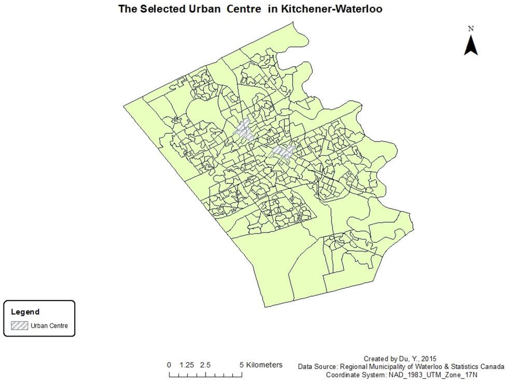
Figure 2.
The Selected Urban Center in Kitchener-Waterloo.
Additionally, a geographically weighted regression model was also applied to study and visualize the spatial non-stationarity for the relations between vegetation, transportation networks, and crime. Unlike those two spatial regression models mentioned above, the geographically weighted regression model is a local-based model. A geographically weighted regression model is a technique for exploring the phenomenon when regression coefficients do not remain stationary over space [65,66,67]. Geographically weighted regressions would be applied to both vegetation and transportation networks. In this study, adaptive kernel type and AICc bandwidth methods were accepted in this study based on the comparison of results.
5. Interpretation of the Relationships between Vegetation, Transportation Network, and Crime: Results
Moran’s I statistics revealed that spatial autocorrelation did exist for residuals obtained from OLS regression and had been reduced by using the spatial lag model (Figure 3 and Figure 4).
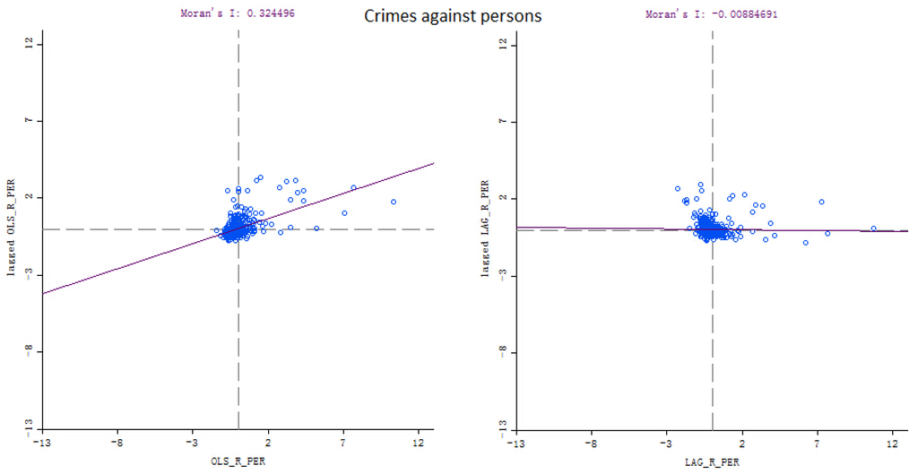
Figure 3.
Moran’s I tests for crimes against persons (OLS: left; Spatial lag: right).
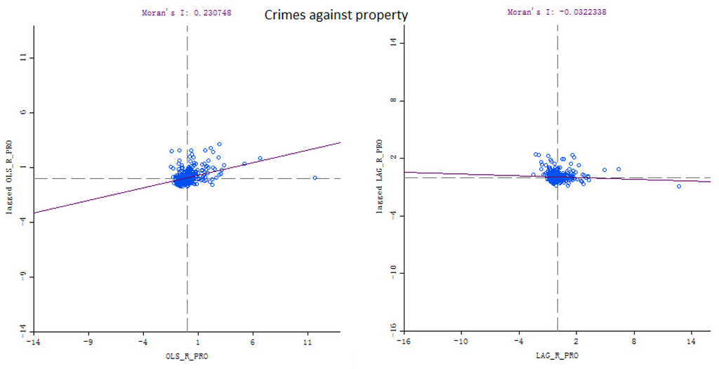
Figure 4.
Moran’s I tests for crimes against property (OLS: left; Spatial lag: right).
For crimes against persons, the value of Moran’s I based on OLS’s residuals was 0.32 and its p-value based on 199 permutations was 0.005, which means the spatial autocorrelation for residuals is highly significant. However, the value of Moran’s I based on the spatial lag model’s residuals could be reduced to −0.009 while its p-value based on 199 permutations was greater than 0.1, which demonstrated that the spatial autocorrelation had been eliminated and was no longer a significant issue. The same situation occurred for crimes against property in that the value of Moran’s I was reduced by using the spatial lag model from 0.23 to −0.03. By testing the spatial autocorrelation for residuals, it could be found that spatial autocorrelation does exist so that the OLS regression model may not be suitable for this study. Residuals’ spatial autocorrelation could be significantly reduced by using the spatial lag model according to Figure 3 for crimes against persons and Figure 4 for crimes against property. Hence, spatial lag models can provide better explanations by taking into account the spatial pattern.
OLS regression models were first employed and then spatial lag models were explored for both crimes against persons and crimes against property. Table 4 presents detailed information for the spatial relationship and the significance of those variables.
Table 4.
Spatial regression results for crimes against persons and crimes against property.
By using OLS regression, only 8.02% of occurrences could be explained for crimes against persons while only 10.31% of occurrences could be explained for crimes against property. The value of R-squared could be significantly enhanced by using spatial lag models for both crimes against persons and crimes against property. The value of pseudo R-squared reached 34.23% for crimes against persons and 26.16% for crimes against property. The higher log-likelihood value represents the better model fit and this value has been increased by using the spatial lag model. In spatial lag models, the magnitudes of coefficients are lower than those in OLS models for both vegetation density and transportation network density. For crimes against persons, the magnitude of vegetation density coefficient decreased from −0.0001 to −7.4863 × 10⁻⁵ while the magnitude of transportation network density coefficient increased from 0.0028 to 0.0036. For crimes against property, the magnitude of vegetation density coefficient dropped from −0.0002 to −0.0001 and the magnitude of transportation network density coefficient also decreased (0.0037 vs. 0.0034). A p-value less than 0.01 represents the 99% confidence level while a p-value less than 0.1 only represents the 90% confidence level. For both types of crime, vegetation density remains significant at the 99% confidence level and negatively correlates with these two types of crime, while transportation network density can only retain significance at the 90% confidence level when using the spatial lag model for crimes against property, but is positively associated with both crimes. For other control variables, only single-parent family density can retain significance at the 90% confidence level for crimes against persons and the 95% confidence level for crimes against property. This means that single-parent family density can boost criminal events while population density is not a significant variable for both crimes against persons and crimes against property. Different from the studies from Shaw and McKay [20], Wolfe and Mennis [11], poverty is also not a significant term influencing the distribution of crimes in the Kitchener-Waterloo Region since it retains significance at less than the 90% confidence level for both crimes against persons and crimes against property.
Four specific types of crime were also examined by using the spatial lag model and the diagnostics results are presented in Table 5. The models of assaults and drugs have the greatest explanatory power with the values of pseudo R-squared around 0.30. However, only 15.70% of variation in the vehicle theft density and 13.04% of variation in the sex offence density can be explained by these independent variables in this study.
Table 5.
Spatial regression results for assaults, vehicle thefts, sex offences, and drugs.
These spatial lag model results demonstrate that the spatial lag term is significant for each specific type of crime. However, vegetation density and transportation network density tend to have various impacts on these four types of crime. Transportation network density is significantly and positively correlated with drugs while it is not a significant explanatory variable for assaults, vehicle thefts and sex offences. Vegetation density is significant at the 99% confidence level for vehicle thefts and significant at the 95% confidence level for assaults and drugs. Additionally, vegetation density is not a significant variable for sex offences. The relationship between vegetation density and crime remains negative. The greatest magnitude of vegetation density coefficient appears for drugs while the transportation network density also has the greatest impact on drugs. As for other socio-economic and socio-demographic control variables, single-parent family density retains significance for assaults and vehicle thefts while population density is only significant for sex offences (p < 0.1).
The urban dummy variable was also added in the model to examine the differences between urban center and urban periphery. Table 6 and Table 7 present the spatial regression results for crimes against persons, crimes against property, and four specific types of crime.
Table 6.
Spatial regression results for crimes against persons and crimes against property at the urban central-peripheral gradient.
Table 7.
Spatial regression results for assaults, vehicle thefts, sex offences, and drugs along the urban central-peripheral gradient.
By adding this urban dummy variable, the spatial lag model can provide better explanations for either crimes against persons or crimes against property. The value of pseudo R-squared for crimes against persons was enhanced to 0.4120 and the value for crimes against property reached 0.3179. In addition, the value of log likelihood for crimes against persons and crime against property was increased to 3701.33 and 3506.98, respectively, demonstrating that this added urban dummy variable can improve model fit. The spatial lag term remains significant at the 99% confidence level for both models and this added urban dummy variable also remains significant at the 99% confidence level. The significance of transportation network density for crimes against person decreases to the 90% confidence level while it is not even significant at the 90% confidence level for crimes against property. Additionally, the magnitude of the transportation network density coefficient decreases for both crimes against persons and crimes against property. The significance of vegetation density remains at the same confidence level while the magnitude also decreases slightly for both crimes against persons and crimes against property. The magnitudes of the other coefficients were also reduced since the urban dummy variable is known as a significant component of the explanation of crime distribution in this study.
All of these crime distributions except the sex offences distribution can be better explained by adding this urban dummy variable. The value of pseudo R-squared was enhanced to 36.34%, 25.67%, and 34.92% for assaults, vehicle thefts, and drugs, respectively. The value of log likelihood was also improved for assaults, vehicle thefts, and drugs separately, representing the better model fit. The urban dummy variable remains significant (p < 0.01) for all types of crime except for sex offences. Transportation network density is only significant for drugs (p < 0.1), and vegetation density is significant for assaults (p < 0.01), vehicle thefts (p < 0.01) and drugs (p < 0.05). Different from models without an urban dummy variable, population density is significant for assaults, vehicle thefts, and sex offences, while single-parent family density is no longer significant. This spatial lag model with an urban dummy variable was considered as the final model in this study.
The geographically weighted regression model was then employed in this study and independent variables used in this model included poverty density, population density, single-parent family density, vegetation density and transportation network density. The urban dummy variable was not added to the geographically weighted regression models because it had already taken into account the urban center features and hence may influence the results and introduce bias into the coefficient’s distribution. The results of the geographically weighted regression model had smaller AICc values compared to results obtained from OLS regression model for both crimes against persons and crimes against property. Smaller AICc values represent an improvement from 0.0802 to 0.2635 and from 0.1094 to 0.2730 for crimes against persons and crimes against property, respectively. Coefficients of vegetation density and transportation network density obtained from the geographically weighted regression could be seen to provide some insights into the spatial non-stationarity of these explanatory variables. Figure 5 presents the spatial variation of transportation network density’s impact on crimes against persons and Figure 6 presents the different impacts of vegetation density on crimes against persons.
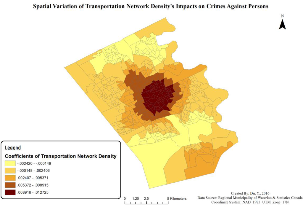
Figure 5.
Transportation network density’s impact on crimes against persons.
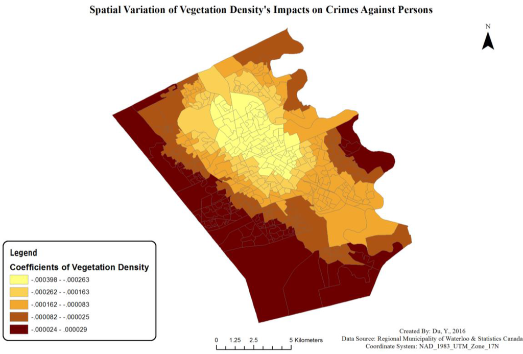
Figure 6.
Vegetation density’s impact on crimes against persons.
The greatest positive relationship between crime and transportation network density tends to occur in uptown Waterloo and downtown Kitchener. Urban central areas selected fall within the boundary representing the highest coefficients. The coefficients of transportation network densities remain positive for almost the whole region while the values of coefficients in peripheral areas appear to be smaller.
Unlike Figure 5, areas drawn in brighter colors represent stronger negative relationships between crime and vegetation density. Vegetation appears to provide more deterrence in the urban center than in the urban periphery. Those selected dissemination areas represented for urban centers also fall within the inner circle associated with the smallest coefficient values, which, in fact, reveal stronger deterrence. Additionally, this negative relationship between vegetation density and crimes against persons remains for almost the whole study region.
Figure 7 and Figure 8 depict the impacts of transportation network density and vegetation density on crimes against property. Their impact on crimes against property appear to be different from their impact on crimes against persons, but there are still some common characteristics.
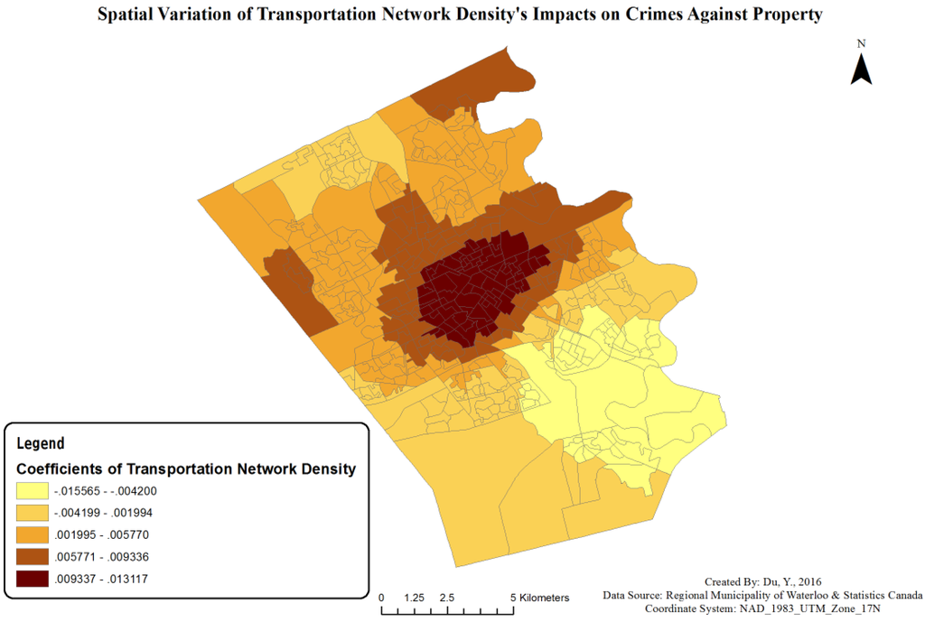
Figure 7.
Transportation network density’s impact on crimes against property.
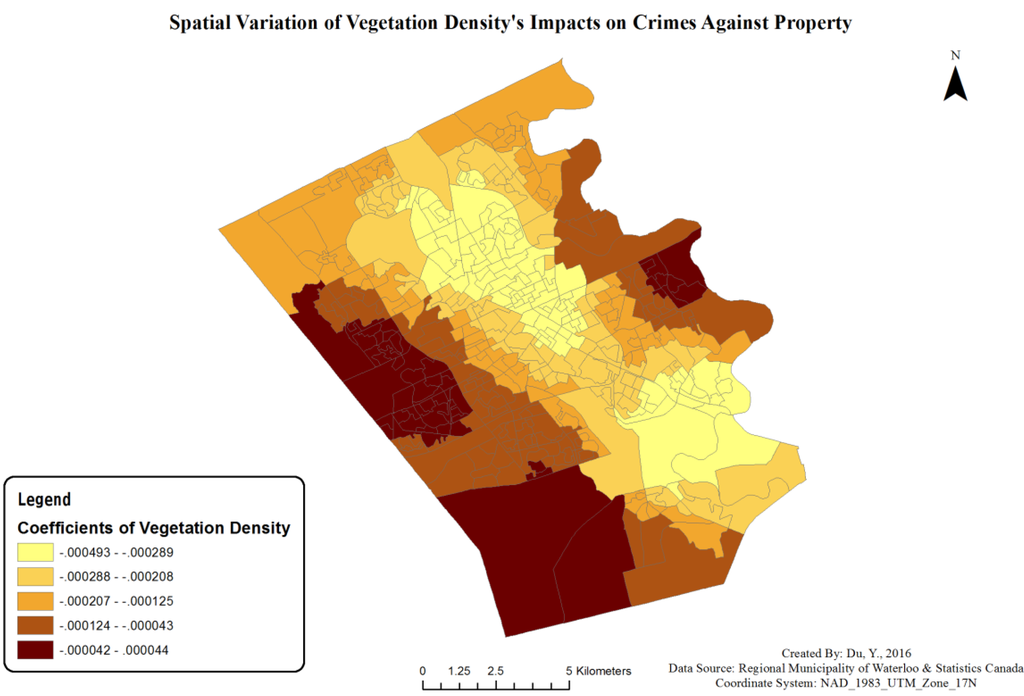
Figure 8.
Vegetation density’s impact on crimes against property.
The general trend depicted in Figure 7 is similar to Figure 5. Some peripheral areas seem to have a greater positive relationship between transportation network density and crime. However, the coefficients of transportation network density in the urban central areas still fall within the highest gradient or the second highest gradient. The coefficients also remain positive among most of the region.
Figure 8 portrays vegetation within the urban center that still has the strongest deterrence to crimes against property. Additionally, another area along with the arterial road also tends to have a greater magnitude of the coefficient. However, vegetation density retains a negative relationship with crimes against property among the whole region.
6. Discussion
The results of this case study suggest an inverse relationship between vegetation and crime, while the relationship between transportation networks and crime retains positive. After controlling other socio-economic and socio-demographic variables, vegetation density still retains a significant negative relationship with both crimes against persons and crimes against property. Meanwhile, transportation network density consistently contributes to occurrences of crimes against persons and crimes against property. Even though different types of tree cover may have various influences on crime, which were not tested in this study, the overall contribution of vegetation to the society appears to be positive based on this study. Vegetation can be a deterrence to criminal events. This result also matches the studies from Wolfe and Mennis [11] and Troy et al. [10]. In addition, even though transportation networks can attract more eyes on the street, it also provides the convergence between offenders and criminal targets. Additionally, transient strangers attracted by transportation networks improve the potential for crime. Transportation networks may have both positive and negative influences on crime in that they tend to have stronger impact on increasing criminal events. Furthermore, both vegetation and transportation networks appear to have a stronger impact on crimes against property. The reason why vegetation has a stronger deterrence for crimes against property may be explained by the “Broken Window” theory, which states that well-maintained green space presents authority, and, hence, crimes against property such as breaking and entering, and vehicle theft, will be reduced. However, transportation networks seem to have a stronger relationship with crimes against persons, and they are not significant for crimes against property. This conclusion may be different from the conclusion supported by Brantingham and Brantingham [43], who found that criminals who targeted property always committed crimes in areas with a completed road network so that they could find ways to easily escape. It may also violate the standpoint of Jarrell and Howsen [44], i.e., that strangers in an area can have significant impact on crimes against property and few influences on crimes against persons. In another words, crimes against property can be more influenced by vegetation and crimes against persons can be more influenced by transportation networks. The spatial lag term is significant for both models. It indicates that spatial cluster does exist and impacts on crime occurrence, making it possible for offenders to easily move from one block to another. The spatial influence may also be explained by reputations of specific areas or referred to ranges of routine activities of perpetrators.
Four specific crime types have also been examined by using spatial lag models. There is no significant relationship between vegetation, transportation networks, and sex offence in this study, and it is probably due to low rates of sex offences happening in this area. Vegetation density has a significant relationship with assaults, vehicle theft and drugs and it may still be associated with the influence of well-maintained green spaces. Additionally, a large proportion of green space tends to attract more people outside and thus provides more surveillance. Transportation network density appears to have a significant positive relationship with assault, but its significance was reduced by adding an urban dummy variable. However, transportation networks impact significantly on the occurrence of drug-relevant crimes. The relationship is consistent with the findings of Weisheit et al. [68], who found that drug trafficking was facilitated by highway improvements. Even though the size of the Kitchener-Waterloo Region tends to be a medium-size region with a relatively low poverty rate, the relationship between vegetation and crime still remains the same as other cities, like Philadelphia [11] and Portland [12], while the relationship between transportation network and crime is the same as other studies in British Columbia, Canada [15].
Spatial analyses, by adding urban dummy variables in spatial regression models, and geographically weighted regression analyses, indicate that urban factors are associated with higher crime density. However, transportation networks still have a stronger positive impact on crimes compared to this urban factor. Based on those visualized results, the impacts of vegetation and transportation networks tend to vary over space. Vegetation appears to be more important in the urban center because it can provide more deterrence than it can provide in the urban periphery. However, vegetation still retains a negative relationship with crime in the urban periphery and this conclusion may be different from the study of Troy et al. [10], in which some positive relationships between vegetation and crime were found in rural areas. Additionally, transportation networks in the urban center can attract more criminals. Perpetrators may still choose the urban center to commit crimes because higher accessibility produced by dense transportation networks can potentially provide perpetrators convenience. Also, land use in the urban center, such as commercial land use [31], may also lead to the difference between the urban center and the urban periphery. In addition, transportation network density and vegetation density have the greatest magnitude not only in the urban center but also in the areas around the arterial roads, which are designated as arterial commercial corridors [63,64]. However, the different impact of commercial and residential land use needs to be further inspected.
There are limitations in this study that could affect its accuracies and conclusions. First, not all variables were considered in this study because of data limitation. Since Statistics Canada’s collection of data in 2011 was totally different from that done in 2006, not all socio-economic datasets in 2011 could be obtained at the dissemination area level. As a consequence, other socio-economic variables such as education and ethnicity cannot be considered in this study even though these variables have proven associations with crime. The impact of these omitted variables may have a significant influence on the results. Also, human mobility has not been considered in this study because of the lack of data pertaining to residents’ activity. A recent study by Mburu and Helbich [69] suggests that the ambient population considering human mobility can improve the analysis of crime. Not only place-based analysis could be conducted for analyzing crime but also direction-based analysis may help explain the occurrence of crime. Furthermore, with limited variables being included, the overall R-squared values were relatively low.
Additionally, these data sources were obtained from different years and this may introduce bias into this study. Even though the majority of land use remained the same during these years, there are still some potential differences for vegetation cover between 2009 and 2013. Moreover, the socio-economic and socio-demographic situations change over time. However, the datasets from 2011 are the latest census datasets that could be obtained. Furthermore, the date of the Landsat imagery employed in this study may also influence the reliability of results since some plant species had not turned green in May, and, hence, that vegetation might have been misclassified.
The classification accuracy of land use maps is another limitation. Since the resolution of the final integrated image was 8 m × 8 m, some areas with trees may not be classified as vegetation. There is no appropriate library land use classification dataset available for the Kitchener-Waterloo Region and the classification map used was the best resource we could obtain. In addition, without the support from high-resolution imagery, vegetation cannot be better classified according to its type and, therefore, further inspection cannot be conducted based on this land use classification map. The calculation of vegetation density based on pixel counting may reduce the accuracy. Some pixels divided by the boundary line had to be counted as a whole for one specific dissemination area only.
The modifiable area unit problem (MAUP) might be another issue. The datasets applied in this study were all at the dissemination area level, which is the smallest statistic spatial unit in Canada. However, other studies may be based on different spatial units. Troy et al. [10] conducted their research based on the census block, which is the smallest spatial unit in US, while Wolfe and Mennis [11] processed their study based on census tracts. The conclusions based on different spatial units may be totally different, while no research has inspected this influence on exploring the relationship between crime and vegetation. We have provided further insight based on this spatial unit, extending previous studies.
7. Conclusions
The findings from this research based on Kitchener-Waterloo provide strong evidence for the relationship between vegetation, transportation networks and crime in a number of ways. First, vegetation retains negative association with both crimes against persons and crimes against property while transportation networks retain a positive relationship with crimes against persons and crime against property. Second, this result holds for both crimes against persons and crimes against property, but vegetation tends to have stronger impacts on crimes against property and transportation networks tends to have stronger impacts on crimes against persons. Third, spatial autocorrelation has been counted and these two spatial relationships remain the same. Fourth, vegetation can be considered a deterrence for assaults, vehicle thefts and drugs, while transportation networks can be a facilitator for drugs. Fifth, urban character affects the spread of crime while urban centers tend to attract more crime. Finally, both vegetation and transportation networks may have a stronger impact in the urban center than in the urban periphery.
These findings address the gap in the literature in terms of the association between vegetation and crime in Canada. However, because of different urban characteristics in different cities, the analyses based on other cities may provide opposite findings and conclusions. The analysis of crime is complicated and should be explored further. Additionally, the relationship between crime and transportation networks can be understood based on neighborhood influences. This study can provide suggestions for better policies for governments and communities.
Acknowledgments
This research was supported by Grant RGPIN-2014-06359 from NSERC and was made possible because of the generous supporter, Jonathan Li, by providing the original datasets. We are also grateful for the help from Weikai Tan and Renfang Liao to generate the classification imagery together.
Author Contributions
Yikang Du is the corresponding author who theoretically proposed and demonstrated the relationship mentioned in this paper and drafted the whole paper; Jane Law contributed greatly to improving the assessment and the manuscript.
Conflicts of Interest
The authors declare no conflict of interest.
References
- Sharpe, B. Geographies of criminal victimization in canada. Can. Geogr. 2000, 44, 418–428. [Google Scholar] [CrossRef]
- Boyce, J.; Cotter, A.; Perreault, S. Police-Reported Crime Statistics in Canada, 2013; Statistics Canada: Ottawa, ON, Canada, 2014. [Google Scholar]
- Andresen, M.A. Crime measures and the spatial analysis of criminal activity. Br. J. Criminol. 2006, 46, 258–285. [Google Scholar] [CrossRef]
- Frank, R.; Andresen, M.A.; Brantingham, P.L. Visualizing the directional bias in property crime incidents for five canadian municipalities. Can. Geogr. 2013, 57, 31–42. [Google Scholar] [CrossRef]
- Anselin, L.; Cohen, J.; Cook, D.; Gorr, W.; Tita, G. Spatial analyses of crime. Crim. Justice 2000, 4, 213–262. [Google Scholar]
- Nasar, J.L.; Fisher, B. ‘Hot spots’ of fear and crime: A multi-method investigation. J. Environ. Psychol. 1993, 13, 187–206. [Google Scholar] [CrossRef]
- Michael, S.E.; Hull, R.B. Effects of Vegetation on Crime in Urban Parks; Virginia Polytechnic and State University: Blacksburg, VA, USA, 1994. [Google Scholar]
- Kuo, F.E.; Sullivan, W.C. Environment and crime in the inner city does vegetation reduce crime? Environ. Behav. 2001, 33, 343–367. [Google Scholar] [CrossRef]
- Snelgrove, A.G.; Michael, J.H.; Waliczek, T.M.; Zajicek, J.M. Urban greening and criminal behavior: A geographic information system perspective. Hort Technol. 2004, 14, 48–51. [Google Scholar]
- Troy, A.; Grove, J.M.; O’Neil-Dunne, J. The relationship between tree canopy and crime rates across an urban–rural gradient in the greater baltimore region. Landsc. Urban Plan. 2012, 106, 262–270. [Google Scholar] [CrossRef]
- Wolfe, M.K.; Mennis, J. Does vegetation encourage or suppress urban crime? Evidence from Philadelphia, pa. Landsc. Urban Plan. 2012, 1082, 112–122. [Google Scholar] [CrossRef]
- Donovan, G.H.; Prestemon, J.P. The effect of trees on crime in Portland, Oregon. Environ. Behav. 2012, 44, 3–30. [Google Scholar] [CrossRef]
- Jacobs, J. The Death and Life of Great American Cities; Vintage: New York, NY, USA, 1961. [Google Scholar]
- Bevis, C.; Nutter, J.B. Changing street layouts to reduce residential burglary. In The Annual Meeting of the American Society Of Criminology; Minnesota Crime Prevention Center: Atlanta, GA, USA, 1977; pp. 1–35. [Google Scholar]
- Beavon, D.J.; Brantingham, P.L.; Brantingham, P.J. The influence of street networks on the patterning of property offenses. Crime Prev. Stud. 1994, 2, 115–148. [Google Scholar]
- Groff, E.R.; Weisburd, D.; Yang, S.M. Is it important to examine crime trends at a local “micro” level? A longitudinal analysis of street to street variability in crime trajectories. J. Quant. Criminol. 2010, 26, 7–32. [Google Scholar] [CrossRef]
- Rephann, T.J. Links between rural development and crime. Pap. Reg. Sci. 1999, 78, 365–386. [Google Scholar] [CrossRef]
- Boggs, S.L. Urban crime patterns. Am. Sociol. Rev. 1965, 30, 899–908. [Google Scholar] [CrossRef] [PubMed]
- Andresen, M.A. A spatial analysis of crime in Vancouver, British Columbia: A synthesis of social disorganization and routine activity theory. Can. Geogr. 2006, 50, 487–502. [Google Scholar] [CrossRef]
- Shaw, C.R.; McKay, H.D. Juvenile Delinquency and Urban Areas: A Study of Rates of Delinquency in Relation to Differential Characteristics of Local Communities in American Cities; University of Chicago Press: Chicago, IL, USA, 1942. [Google Scholar]
- Sampson, R.J.; Groves, W.B. Community structure and crime: Testing social-disorganization theory. Am. J. Sociol. 1989, 774–802. [Google Scholar] [CrossRef]
- Coleman, J.S.; Coleman, J.S. Foundations of Social Theory; Harvard University Press: Cambridge, MA, USA, 1994. [Google Scholar]
- Tseloni, A.; Osborn, D.R.; Trickett, A.; Pease, K. Modelling property crime using the british crime survey. What have we learnt? Br. J. Criminol. 2002, 42, 109–128. [Google Scholar] [CrossRef]
- Wilson, W.J. When Work Disappears: The World of the New Urban Poor; Vintage: New York, NY, USA, 2011. [Google Scholar]
- Pattillo, M. Black Picket Fences: Privilege and Peril among the Black Middle Class; University of Chicago Press: Chicago, IL, USA, 2013. [Google Scholar]
- Cohen, L.E.; Felson, M. Social change and crime rate trends: A routine activity approach. Am. Sociol. Rev. 1979, 588–608. [Google Scholar] [CrossRef]
- Newman, O. Defensible Space; Macmillan: New York, NY, USA, 1972. [Google Scholar]
- Johnstone, J.W. Social class, social areas and delinquency. Sociol. Soc. Res. 1978, 63, 49–72. [Google Scholar]
- Smith, W.R.; Frazee, S.G.; Davison, E.L. Furthering the integration of routine activity and social disorganization theories: Small units of analysis and the study of street robbery as a diffusion process. Criminology 2000, 38, 489–524. [Google Scholar] [CrossRef]
- Bursik, R.J., Jr.; Grasmick, H.G. Neighborhoods & Crime; Lexington Books: Lanham, MD, USA, 1999. [Google Scholar]
- Chen, D.; Weeks, J.R.; Kaiser, J.V., Jr. Remote sensing and spatial statistics as tools in crime analysis. Geogr. Inf. Syst. Crime Anal. 2005. [Google Scholar] [CrossRef]
- Weisel, D.L. Addressing Community Decay and Crime: Alternative Approaches and Explanations; The Urban Institute: Washington, DC, USA, 1994. [Google Scholar]
- Talbot, J.F.; Kaplan, R. Needs and fears: The response to trees and nature in the inner city. J. Arboric. 1984, 10, 222–228. [Google Scholar]
- Shaffer, G.S.; Anderson, L.M. Perceptions of the security and attractiveness of urban parking lots. J. Environ. Psychol. 1985, 5, 311–323. [Google Scholar] [CrossRef]
- Michael, S.E.; Hull, R.B.; Zahm, D.L. Environmental factors influencing auto burglary a case study. Environ. Behav. 2001, 33, 368–388. [Google Scholar] [CrossRef]
- Kuo, F.E. The role of arboriculture in a healthy social ecology. J. Arboric. 2003, 29, 148–155. [Google Scholar]
- Coleman, A. Utopia on Trial: Vision and Reality in Planned Housing; Longwood Pr Ltd.: London, UK, 1985. [Google Scholar]
- Wilson, J.Q.; Kelling, G.L. Broken windows. Atl. Mon. 1982, 249, 29–38. [Google Scholar]
- Kaplan, S. Mental Fatigue and the Designed Environment; Public Environments: Ottawa, ON, Canada, 1987. [Google Scholar]
- Tobias, J.J. Urban Crime in Victorian England; Schocken: New York, NY, USA, 1972. [Google Scholar]
- Brantingham, P.L.; Brantingham, P.J. Nodes, paths and edges: Considerations on the complexity of crime and the physical environment. J. Environ. Psychol. 1993, 13, 3–28. [Google Scholar] [CrossRef]
- Taylor, M.; Nee, C. Role of cues in simulated residential burglary-a preliminary investigation. Bir. J. Criminol. 1988, 28, 396–401. [Google Scholar]
- Brantingham, P.L.; Brantingham, P.J. Criminality of place. Eur. J. Crim. Policy Res. 1995, 3, 5–26. [Google Scholar] [CrossRef]
- Jarrell, S.; Howsen, R.M. Transient crowding and crime. Am. J. Econ. Sociol. 1990, 49, 483–494. [Google Scholar] [CrossRef]
- Costello, A.; Wiles, P. Gis and the journey to crime: An analysis of patterns in south yorkshire. In Mapping and Analysing Crime Data: Lessons from Research and Practice; CRC Press: Boca Raton, FL, USA, 2001; pp. 27–60. [Google Scholar]
- Pyle, G.F.; Hanten, E.W.; Williams, P.G.; Pearson, A.; Doyle, J.G. The Spatial Dynamics of Crime; University of Chicago, Department of Geography: Chicago, IL, USA, 1974. [Google Scholar]
- Natural Resources Canada. Land Cover, Circa 2000-Vector (lcc2000-v)—040p—Kitchener, Ontario; Natural Resources Canada: Ottawa, ON, Canada, 2009. [Google Scholar]
- Service, W.R.P. Waterloo Regional Police Service (WRPS) Annual Report 2013; Waterloo Regional Police Service: Waterloo, ON, Canada, 2014. [Google Scholar]
- Statistics Canada. Table 4 Police-Reported Crime Rate, by Census Metropolitan Area, 2013; Statistics Canada: Ottawa, ON, Canada, 2014. [Google Scholar]
- Breiman, L. Random forests. Mach. Learn. 2001, 45, 5–32. [Google Scholar] [CrossRef]
- Pal, M. Random forest classifier for remote sensing classification. Int. J. Remote Sens. 2005, 26, 217–222. [Google Scholar] [CrossRef]
- Friedl, M.A.; Brodley, C.E. Decision tree classification of land cover from remotely sensed data. Remote Sens. Environ. 1997, 61, 399–409. [Google Scholar] [CrossRef]
- Paola, J.D.; Schowengerdt, R.A. A review and analysis of backpropagation neural networks for classification of remotely-sensed multi-spectral imagery. Int. J. Remote Sens. 1995, 16, 3033–3058. [Google Scholar] [CrossRef]
- Harries, K. The ecology of homicide and assault: Baltimore city and county, 1989–1991. Stud. Crime Crime Prev. 1995, 4, 44–60. [Google Scholar]
- Bottoms, A.; Wiles, P. Crime and housing policy: A framework for crime prevention analysis. In Communities and Crime Reduction; HMSO: London, UK, 1988; pp. 84–98. [Google Scholar]
- Cahill, M.E.; Mulligan, G.F. The determinants of crime in tucson, arizona1. Urban Geogr. 2003, 24, 582–610. [Google Scholar] [CrossRef]
- Canada, S. Low Income in Canada—A Multi-Line and Multi-Index Perspective. Available online: http://www.statcan.gc.ca/pub/75f0002m/2012001/summary-sommaire-eng.htm (accessed on 15 August 2015).
- Dismuke, C.; Lindrooth, R. Ordinary least squares. In Methods and Designs for Outcomes Research; ASHP: Bethesda, MD, USA, 2006; pp. 93–104. [Google Scholar]
- Anselin, L. Exploring Spatial Data With Geoda: A Workbook. Available online: http://www.unc.edu/~emch/gisph/geodaworkbook.pdf (accessed on 15 August 2015).
- Anselin, L.; Hudak, S. Spatial econometrics in practice: A review of software options. Reg. Sci. Urban Econ. 1992, 22, 509–536. [Google Scholar] [CrossRef]
- Ward, M.D.; Gleditsch, K.S. Spatial Regression Models; Sage: London, UK, 2008. [Google Scholar]
- Waterloo, R.O. Regional Official Plan. Available online: http://www.regionofwaterloo.ca/en/regionalGovernment/PreviousROP.asp (accessed on 15 August 2015).
- City of Waterloo. The City of Waterloo Official Plan Land Use Plan Schedule ‘a’; City of Waterloo: Waterloo, ON, Canada, 2013. [Google Scholar]
- City of Kitchener. City of Kitchener Municipal Plan Map 7 Downtown Land Use Districts; City of Kitchener: Kitchener, ON, Canada, 2006. [Google Scholar]
- Brunsdon, C. Geographically weighted regression: A natural evolution of the expansion method for spatial data analysis. Environ. Plan. A 1998, 30, 1905–1927. [Google Scholar] [CrossRef]
- Brunsdon, C.; Fotheringham, S.; Charlton, M. Geographically weighted regression. J. R. Stat. Soc. Ser. D 1998, 47, 431–443. [Google Scholar] [CrossRef]
- Bernasco, W.; Elffers, H. Statistical analysis of spatial crime data. In Handbook of Quantitative Criminology; Piquero, A.R., Weisburd, D., Eds.; Springer: New York, NY, USA, 2010; pp. 699–724. [Google Scholar]
- Weisheit, R.A.; Falcone, D.N.; Wells, L.E. Rural Crime and Rural Policing; US Department of Justice, Office of Justice Programs, National Institute of Justice: Washington, DC, USA, 1994.
- Mburu, L.W.; Helbich, M. Crime risk estimation with a commuter-harmonized ambient population. Ann. Am. Assoc. Geogr. 2016, 106, 804–818. [Google Scholar] [CrossRef]
© 2016 by the authors; licensee MDPI, Basel, Switzerland. This article is an open access article distributed under the terms and conditions of the Creative Commons Attribution (CC-BY) license (http://creativecommons.org/licenses/by/4.0/).