Article

Land Surface Water Mapping Using Multi-Scale Level Sets and a Visual Saliency Model from SAR Images

1
State Key Laboratory of Information Engineering in Surveying, Mapping and Remote Sensing, Wuhan University, Wuhan 430079, China
2
National Disaster Reduction Center of China, NO.6 GuangBaiDongLu, Chaoyang District, Beijing 100124, China
*
Author to whom correspondence should be addressed.
These authors contributed equally to this work.
ISPRS Int. J. Geo-Inf. 2016, 5(5), 58; https://doi.org/10.3390/ijgi5050058
Submission received: 5 January 2016 / Revised: 25 March 2016 / Accepted: 18 April 2016 / Published: 5 May 2016
(This article belongs to the Special Issue Advances and Innovations in Land Use/Cover Mapping)

Abstract

:
Land surface water mapping is one of the most basic classification tasks to distinguish water bodies from dry land surfaces. In this paper, a water mapping method was proposed based on multi-scale level sets and a visual saliency model (MLSVS), to overcome the lack of an operational solution for automatically, rapidly and reliably extracting water from large-area and fine spatial resolution Synthetic Aperture Radar (SAR) images. This paper has two main contributions, as follows: (1) The method integrated the advantages of both level sets and the visual saliency model. First, the visual saliency map was applied to detect the suspected water regions (SWR), and then the level set method only needed to be applied to the SWR regions to accurately extract the water bodies, thereby yielding a simultaneous reduction in time cost and increase in accuracy; (2) In order to make the classical Itti model more suitable for extracting water in SAR imagery, an improved texture weighted with the Itti model (TW-Itti) is employed to detect those suspected water regions, which take into account texture features generated by the Gray Level Co-occurrence Matrix (GLCM) algorithm, Furthermore, a novel calculation method for center-surround differences was merged into this model. The proposed method was tested on both Radarsat-2 and TerraSAR-X images, and experiments demonstrated the effectiveness of the proposed method, the overall accuracy of water mapping is 98.48% and the Kappa coefficient is 0.856.

1. Introduction

Water resources are an irreplaceable strategic resource for human survival. Land surface water (LSW) is an important part of the water cycle. LSW mapping, using remote sensing techniques, plays an important role in wetland monitoring, flood monitoring, flood disaster assessment, surface water area estimation, and water resources management. Although multi-spectral optical images have been found to be effective when the sky is clear, there are some limitations in overcast weather conditions. However, due to their capabilities of large-area coverage, cloud penetration and all-weather acquisition, the SAR image data could compensate for the weakness in optical images in such conditions for LSW mapping [1]. This paper proposes a fast and reliable land surface water mapping method of large-area and high-resolution SAR images. Only calm water was considered including calm rivers and lakes, not including puddles and paddy fields.
Water classification is a particular case of SAR image classification, with only two classes to assign; it is widely used in applications such as wetland monitoring, flood monitoring, surface water area estimation and so on. However, due to the presence of coherent speckle, which can be modeled as strong, multiplicative noise, segmentation of SAR images is generally acknowledged as a difficult problem [2]. Up to now, many segmentation algorithms have been proposed ,such as the threshold method [3], edge detection method [4,5], region-based method [6], and fuzzy-based method [7]. In addition, in the recent research, Markov random fields (MRFs) and active contour models (ACMs) are two of the most useful methods for SAR image segmentation. As concerns the MRF segmentation method, Deng et al. [8] proposed a novel Markov random field (MRF) model to generate accurate unsupervised sea and ice segmentation results. Stéphane and Grégoire [9] developed a vector hidden Markov chain (HMC) model that was adapted to a multi-scale description to segment oil slick from sea SAR images. Gan et al. [10] and Wang et al. [11] proposed an unsupervised SAR image segmentation method based on Triplet Markov Fields, respectively. After that, A Reversible Jump Markov Chain Monte Carlo scheme is designed to simulate the SAR image segmentation model [12]. As concerns the active contour models method, Huang et al. [13] used a partial differential equation (PDE)-based level set method for oil slick segmentation in SAR images. Silveira and Heleno [14] adopted a mixture of lognormal densities for SAR image segmentation between water and land, and results demonstrated the good performance of their proposed method. Moreover, a novel level set segmentation method that uses a heterogeneous clutter model is proposed to overcome the problem of strong speckle and texture in fine spatial resolution SAR images [15]. Yin and Yang [16] investigates the application of a level set method for the automated multiphase segmentation of multiband and polarimetric synthetic aperture radar (SAR) images.
However, these segmentation methods cannot be used directly for water segmentation in SAR images because of the following reasons: (1) Most of these segmentation methods are not designed for water segmentation in SAR images, as water features in SAR images are not considered; moreover, there are also some problems in the existing segmentation methods. For example, the edge detection technique is plagued by difficulties that include discontinuous boundary points and a pseudo-boundary in the homogeneous region, which cause significant difficulties in subsequent processing. The region-growing approach is user-dependent during the growing and merging of neighboring small regions, while segmentation methods based on the thresholding of grey levels are often inappropriate for SAR images because of the presence of speckle noise. The MRF method has a large computational cost and hence is not widely used in practice, especially for large-area images; (2) The geometric ACMs, known as level sets [17], have the advantage of being independent from parameterization and are able to automatically change topology. In the level set method, a curve is embedded as a zero level set of a higher dimensional surface. Next, the entire surface is evolved to minimize a metric defined by the curvature and image gradient, i.e., the speed terms of the level set will reduce to zero when reaching the object boundary. Although level set methods present a good performance in SAR image segmentation, there are still some problems. The curve in level sets is usually evolved on the whole SAR image, so objects other than the water body are also extracted. In particular, the segmentation results for large-area images at a high spatial resolution often yield a wide variety of very small-scale image objects (i.e., “salt and pepper” effects); (3) Objects with a low radar cross section similar to calm water, such as roads, airstrips, radar shadows, or paddy fields, may affect the results of water extraction.
Water regions are salient objects in SAR images because these regions often occupy a large area and appear as the darkest grey value; therefore, human eyes usually focus their initial attention on water regions. Selective visual attention is a mechanism by which we can rapidly direct our gaze towards objects of interest in our visual environment, and ignore some information that is not important [18]. This mechanism reduces the calculation time during information processing. Thus, the introduction of this mechanism into the processing of remote sensing images could significantly improve its efficiency. Recently, Itti et al. [19] proposed a classical model of selective visual attention, and this model can be used to search for salient objects in complex scenes. Since then, many objects detection methods have been developed using this model. For example, Itti et al. [20] applied this model to a wide range of target detection tasks, using synthetic and natural stimuli. Walther et al. [21] proposed a method for detecting multiple objects in cluttered scenes based on a bottom-up visual attention model. Li et al. [22] proposed a wavelet transform saliency model for generating a saliency map to detect natural objects. Gao et al. [23] presented a novel detection model based on a visual attention mechanism to detect ships in remote sensing images. Li and Itti [24] integrated saliency features acquired by a visual salience model, and with gist features, to detect objects, such as ships, buildings and airplanes in remote sensing images. However, these models are aimed at analyzing images of nature or at extracting ships, airplanes, etc. from optical satellite images, and they are not designed for SAR images which make it difficult to apply them directly.
The main purpose of this paper is to propose a fast and accurate land surface water mapping method, and most important is that it can solve some complex situation, such as shadow, farmland confusion, etc. The remainder of this paper is structured as follows. In Section 2, our method is formulated and applied to SAR image water extraction. Firstly, a TW-Itti model is proposed. Secondly, we describe the adaptive multi-scale level set method based on Gamma model. Thirdly, a post-processing method is described. Some experimental results are shown in Section 3, before we conclude the paper in Section 4.

2. Proposed Method

Given the above problems, a novel water segmentation method was proposed based on the integration of multi-scale level sets and a visual salience model, as follows, (1) To improve the accuracy and efficiency of water extraction, the classic Itti model is first introduced to detect the SWR. After that, the level set method can be applied only to these regions, and at the same time, the visual salience map can be used for initializing the zero level set function. Thus, we can detect water regions rapidly using Itti model and we can accurately segment water from those regions using level sets; (2) The classical Itti model is not designed for SAR water images, thus, an improved visual saliency attention model was presented. First, we replace the color images in the Itti model with textured images, which are generated using the gray-level co-occurrence matrix (GLCM) algorithm. Based on the grey values of the water body, a weight coefficient is introduced to calculate the center-surround differences; (3) In order to better avoid “salt and pepper” effects, multi-scale technology is introduced in the level sets method. A multi-scale level set method was proposed by Sui et al. [25], the difference with our approach being that we use OTSU algorithms [26] to adaptively define the initial level set function; (4) To detect objects that may be confused with calm water, a post-processing method was proposed based on object-oriented geometrical features.
In this section, the framework of our rapid water extraction method for SAR imagery was presented, as shown in Figure 1.
The principal steps of our method are as follows.
Step 1: Generate a visual salience map using the improved Itti model.
Step 2: Decompose the original image and visual saliency map into L scales by the bilinear interpolation algorithm. Let K = L.
Step 3: SWR regions are obtained: segment the saliency map into binary images at each scale using the OTSU method, and then objects in these binary images can be marked using the connecting area algorithm. Next, SWR regions (black rectangles in the SAR image shown in Figure 1) can be obtained by calculating the maximum external rectangle of each marked object.
Step 4: Use the OTSU algorithms to initialize the level set function at scale L. Obtain the scale K segmentation results using the level set method with the Gamma model.
Step 5: K = K − 1. If K ≥ 0, return to Step 4, until the final segmentation result is obtained.
Step 6: Post-processing: the weighting of the smoothness within the shape is applied to the final binary image to distinguish paddy fields from rivers or lakes (see Section 2.3).

2.1. Improved TW-Itti Model

The model proposed in this paper draws its inspiration from the bottom-up attention model proposed by Itti et al. [20] (see the left part of Figure 1). Our contribution is focused mainly on the extraction of early visual features. Instead of using color information, the textures generated by the GLCM are applied to obtain the feature maps. Since we used single-polarized and single-band SAR images, no colors can be acquired; thus, we fused the texture feature to generate color images. The benefit of doing this is to enhance the visibility of the water body and the background. Moreover, in view of the dark grey value of water, a new calculation method for center-surround differences is presented. Center-surround is implemented in the model as the difference between fine and coarse scales, The center is a pixel at scale c { 2 , 3 , 4 } , and the surround is the corresponding pixel at scale s = c + δ , with δ { 3 , 4 } . The across-scale difference between two maps, denoted “ ” below, is obtained by interpolation to the finer scale and point-by-point subtraction. The input is provided as a static gray image, and nine spatial scales are generated using dyadic Gaussian pyramids, which progressively low-pass filter and subsample the input image. I is used to create a Gaussian pyramid I(σ), where σ∈(0…8) is the scale. The center-surround differences (   defined previously) between a“center” fine scale c and a “surround” coarser scale s yield the feature maps.
The first set of feature maps is concerned with intensity contrast, which, in mammals, is detected by neurons sensitive either to dark centers on bright surrounds or to bright centers on dark surrounds. Here, both types of sensitivities are simultaneously computed (using a rectification) in a set of six maps I ( c , s ) .
I ( c , s ) = | I ( c ) I ( s ) | ,   c { 2 , 3 , 4 } , s = c + σ , σ { 3 , 4 }
Considering the dark grey value of water, a weight coefficient is introduced to calculate the center-surround differences, mainly to maintain the low reflective value of water. Thus, Equation (1) can be rewritten as below:
I ( c , s ) = | ω · I ( c ) I ( s ) |
where ω is the weight coefficient and ω [ 0 , 1 ] .
A second set of maps is similarly constructed for the texture channels. A texture image T is generated using GLCM and principal components analysis (PCA) algorithm. Here, T is comprised of five conventional textures, i.e., energy, correlation, inertia, entropy and inverse difference moment).The window size is 7 × 7, the distance value is 1 pixel and there are 16 grey levels. After acquiring these textures, the PCA method is used to obtain the first principal component that represents texture image T. The texture feature maps T(c,s) can be represented as follows:
T ( c , s ) = | T ( c ) T ( s ) |
The GLCM-based features, proposed by Haralick et al. [27], have been used widely in texture segmentation. They are defined for the neighborhood of an input image and represented by using the second order joint condition probability density pij, which is the relative frequency at which two image pixels are related. The construction of the GLCM depends on three parameters, i.e., the relative distance ( d ), the window size ( w ), and the orientation ( θ ) between pixels in a pair. In this paper, the distanced is set to one pixel, the window size is set to 7 × 7 pixels, while the orientation is equal to the average value of four directions ( 0 ° ,   45 ° ,   90 ° and 135 ° ). Next, we extract five features from the GLCM, as follows:
Energy:
A S M = i j P ( i , j ) 2
Correlation:
C O N = [ i j ( ( i j ) p ( i , j ) u x u y ) ] / σ x σ y
Inertia:
I N T = i j ( i j ) 2 p ( i , j )
Entropy:
E N T = i j p ( i , j ) log p ( i , j )
Inverse Difference Moment
I D M = i j 1 1 + ( i j ) 2 p ( i , j )
where u x ,   u y ,   σ x ,   σ y are the means and standard deviations of the marginal distribution associated with P ( i , j ) / R , and R is a normalizing constant.
After acquiring these five texture features, they are fused using PCA where the principal components are then used for segmentation purposes. Finally, the fuzzy-C means algorithm is performed with the first three principal components during image segmentation.
The third set of maps is the local orientation   O , here O is obtained from I using oriented Gabor pyramids   O ( σ , θ ) , where σ ( 0 8 ) represents the scale and θ { 0 ° , 45 ° , 90 ° , 135 ° } is the preferred orientation. The orientation feature maps,   O ( c , s , θ ) , are encoded as a group, with a local orientation contrast between the center and surround scales, as follows:
O ( c , s , θ ) = | O ( c , θ ) O ( s , θ ) |
In total, 36 feature maps were computed: six for intensity, six for texture, and 24 for orientation. After processing of across-scale combinations, normalization and linear combinations with six for intensity, six for texture, and 24 for orientation. As mentioned in [20], the improved salience map is generated.
After obtaining the saliency map, suspected water regions can be found by using the Otsu method. The Otsu algorithm is a nonparametric and unsupervised method of automatic threshold selection for image segmentation, and it is a classical method for optical image segmentation. However, due to the strong speckle noise of SAR images, especially for fine spatial resolution SAR images, Otsu method could be invalidated. Thus, it was applied to the visual saliency map, which has no speckle noise, and it is used to segment the visual saliency map and obtain the suspected water regions. At the same time, we can also use this segmentation result of the visual saliency map to initialize the zero level set function, supposing the segmentation result of the visual saliency map is t ( x ) .The details for using the visual saliency map to initialize the zero level set function can be seen in the last part of Section 2.2.

2.2. Adaptive Multi-Scale Level Set Method Based on the Gamma Model

In order to remove the influence of speckle and preserve important structural information, a multi-scale level set algorithm is introduced. We acquire multi-scale images at several scales by decomposing the SAR image using the block averaging algorithm. Because the Gamma model can well represent the distribution of SAR images if the speckle is fully developed and spatially uncorrelated, and the radar backscatter of the region is constant, it is employed to define the energy functional of the level set function for the original SAR image. Even if there is correlation between neighboring pixels, or the radar backscatter features texture, the Gamma distribution can still be used as an approximation by adjusting the number of looks L. For scale images decomposed by the block averaging algorithm, the probability density function (PDF) of the pixel intensity can be also given by a Gamma distribution. For a given image u ( x ) , u ˜ ( x ) is the decomposed image generated by block averaging algorithm. If   u ( x ) is modeled by a Gamma distribution as   u ( x ) ~ Γ ( μ , L ) , then u ˜ ( x ) ~ Γ ( μ , 4 L ) . After using the threshold level set initialization method at the coarsest scale, the initial segmentation result, which is marked by a label, is generated. This label is used not only for the level set initialization at finer scales but also as an additional constraint to guide contour evolution. Consequently, the finest scale image is extracted as the final result.
Chan and Vese [17] proposed a model that implemented the Mumford–Shah functional via the level set function for the purpose of bimodal segmentation. The segmentation is performed using an active contour model without boundaries. Let Ω be a bounded open subset of R 2 , with Ω being its boundary. Let u 0 ( x , y ) : Ω ¯ R be a given image, and C be a curve in the image domain Ω . Segmentation is achieved via the evolution of curve C , which is the basic idea of the active contour model. In the level set method, C Ω is represented by the zero level set of a Lipschitz function ϕ : Ω R , and we replace the unknown variable C with the unknown variable   ϕ .
In this paper, assume that the image is partitioned into two classes Ω 1 and Ω 2 , which are separated by a curve C , and that classes Ω 1 and Ω 2 are modeled using the probability density functions (pdfs) P 1 and P 2 , respectively.
The partition is obtained by minimizing the following energy function:
F ( C , p 1 , p 2 ) = μ L e n g t h ( C ) λ 1 Ω ( log p 1 d x ) λ 2 Ω ( log p 2 d x )
A gamma model was used for high resolution SAR image segmentation. Suppose u SAR ( x , y )   is a SAR image, we model the image in each region Ri by a Gamma distribution of mean intensity ui and number of looks L:
P ( u SAR ( x , y ) ) = L L u i Γ ( L ) ( u SAR ( x , y ) u i ) L 1 e L u SAR ( x , y ) u i
Using the Heaviside function H, and the one-dimensional Dirac function δ0, which are defined, respectively, by
H ( z ) = { 1 if   z 0 0 if   z < 0   and   δ ( z ) = d H ( z ) d z
The segmentation is performed via the evolution of ϕ by minimizing the following energy function:
F ( , p 1 , p 2 ) = μ H ( ) d x λ 1 H ( ) log p 1 d x λ 2 ( 1 H ( ) ) log p 2 d x
where μ , λ 1 , λ 2 are non-negative weighted parameters. Function represents class   Ω 1   for > 0 , and Ω 2   for   < 0 .
The evolution of   ϕ is governed by the following partial differential motion equation:
ϕ t = δ ε ( ϕ ) [ μ   div ( ϕ | ϕ | ) + v + λ 1 log p 1 ( y | θ ^ 1 ) + λ 2 log p 2 ( y | θ ^ 2 ) ]
where δ ε ( ϕ )   is a regularized version of the Dirac function.
Next, we aim to estimate the Gamma parameters θ = {μi}. Using maximum likelihood estimation θ * = arg max θ log p ( y | θ ) . Assuming that the samples y j , j = 1 , , N in each region are independent and identically distributed, the log likelihood is log p ( y | θ ) = log j = 1 N p ( y j | θ ) = j = 1 N log p ( y j | θ ) . Taking the derivative of log p ( y | θ ) with respect to θ and setting them equal to zero, μ i = j = 1 N i y j / N i was obtained, where N i is the pixel number in Ω i .
As we know that the segmentation result of the visual saliency map is t ( x ) , then we simply initialize the level set function ϕ as follows:
ϕ = t ( x )
The main step of the level sets method is as follows (also see the details for Step 4 of our method):
(1)
Initialize the level set function using Equation (15);
(2)
Evolve the level set function ϕ according to Equations (13) and (14);
(3)
Check whether the evolution is stationary. If not, return to Step 2.

2.3. Post-Processing: Using Object-Oriented Geometrical Feature

Water objects in SAR images are continuous regions with low light, and some objects with a low radar cross-section similar to calm water, such as urban roads, airstrips, building shadows or paddy fields, may influence the results of water extraction.
Compared with a large water area, urban roads, airstrips and building shadows are not significant, thus, these areas are ignored after we acquire the SWR regions using the visual salience model. However, some paddy fields remain as salient objects because of their occupation of large areas. In this study, geometrical features are used for post-processing to distinguish paddy fields from water bodies. First, a fast pixel labeling method is applied to search for connected areas in binary images (more details can be found in [28]). Then, the attributes of each object can be acquired, such as the area, perimeter and number of objects. In SAR images, the geometrical features of paddy fields usually appear as regular rectangles, whereas, water bodies such as rivers and lakes, mostly appear as irregular geometrical shape. Thus, inspired by the user guide of eCognition software (Definiens AG, Munich, Germany) [29], the weighting of smoothness (WS) within the shape was introduced to distinguish paddy fields from water bodies, as shown in Equation (16).
W S = Area of Minimum Enclosing Rectangle Area of the object
We obtained good segmentation results using the proposed method, and most paddy fields had geometrical shapes such are as shown in Figure 2a. However, after the evolution of the level sets, some paddy fields were connected each other, such as the shape shown in Figure 2b. Figure 2c shows the object shape of a river and Figure 2d shows the object shape of a lake. The red dashed rectangles are the minimum enclosing rectangles for each object. During image segmentation, the ratio of the minimum enclosing rectangle’s area and the object’s area is used to make the segmentation object’s shape more regular, and the value of the ratio is very close to 1, so the object’s shape is very close to a rectangle. The ratio values for Figure 2a–d are 1.344, 2.143, 6.524 and 2.5869, respectively. Thus, based on the experience value (3000 objects with 15 images were tested), we assume that an object is “water class”, if the value of smoothness weighting in an object is greater than 2, and all others water classes can be removed during post-processing.

3. Experimental Data Set

SAR amplitude images (Radarsat2 and TerraSAR-X) of river basin regions in China were used in the experiment, detailed descriptions of the experiment data can be seen in Table 1.
(1)
Study Area of Huai River: Huai River catchment around eastern China is taken as one of the study areas. The Radarsat 2 images (VV polarization) at a spatial resolution of 3 m were acquired on 7 December 2009. A Google map image of 0.5m resolution with the same region and same season is used as the true water class image, then manual water extraction in this google image is used for reference to check the accuracy of the water extraction process.
(2)
Study Area of Hanjiang and Changjiang River: Hanjiang River is the largest branch of Changjiang River, and they are located in Wuhan City, Hubei Province, China. The TerraSAR-X images (VV polarization) at a spatial resolution of 1 m were acquired on 9 October 2008. A vector map of the same region supported by Map Institute of Hubei Province is used for reference to check the accuracy of the water extraction process.

4. Results and Discussion

The following three methods were compared to evaluate the performance of the proposed method.
ALG1: A MRF segmentation method proposed by Picco and Placio [30].
ALG2: A method for the separation of land and water in SAR images which was proposed by Silveira and Heleno [14].
ALG3: A multi-scale level set method for SAR image segmentation which was proposed by Sui et al. [25].
Note that all of our images were tested without a filter when using the proposed method and the scale level was 2. The value of the smooth index WS = 2, i.e., if the value of the object smoothing index was less than 2, this object could be removed. The weight coefficient of the center-surround differences ω is equal to 0.1.

4.1. Experiment on Radarsat-2 Image

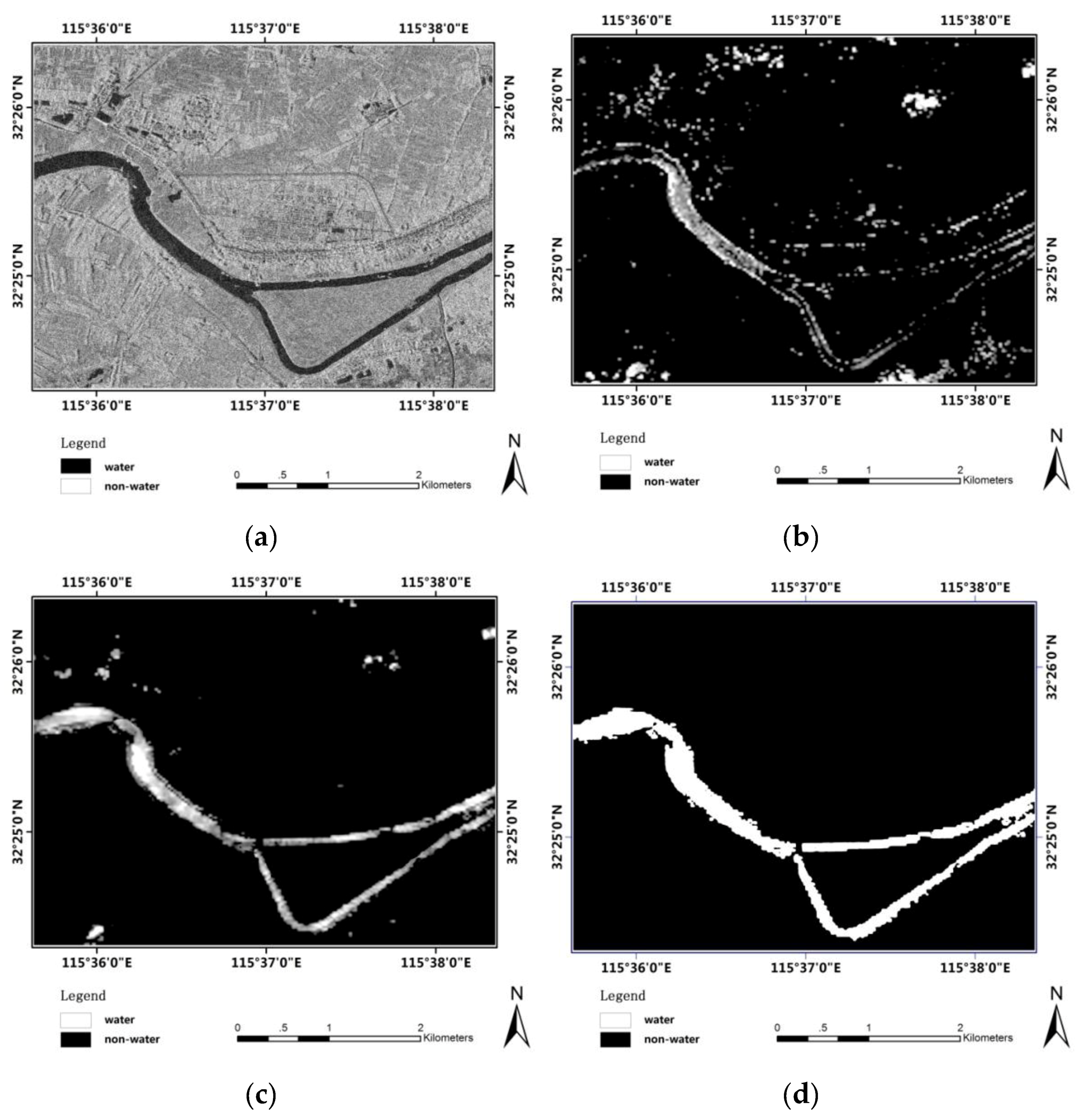
Figure 3 compares the salience maps generated using the Itti model and our model. This shows clearly that our model readily distinguished areas of water. Figure 3a shows the Huai River in eastern China, which was acquired by Radarsat-2 in 2009 in descending VV polarization mode, with a resolution of 3 m and a size of 3024 × 2263 pixels. Figure 3b,c shows the saliency map generated using Itti model and our TW-Itti model, respectively. The experiment validates our model performance much better than the Itti model. In Figure 3b, except for water body, other features are also incorrectly considered to be salient, which made the water body discontinuous. Figure 3d shows the Otsu segmentation result after the post-processing of Figure 3c. It can be seen from Figure 3d that segmentation using the saliency map can acquire main outlines, however, missing edge details. It can be seen that the edges are jagged and irregular. As such, we need to apply the level set method to refine the edge and make it smooth.
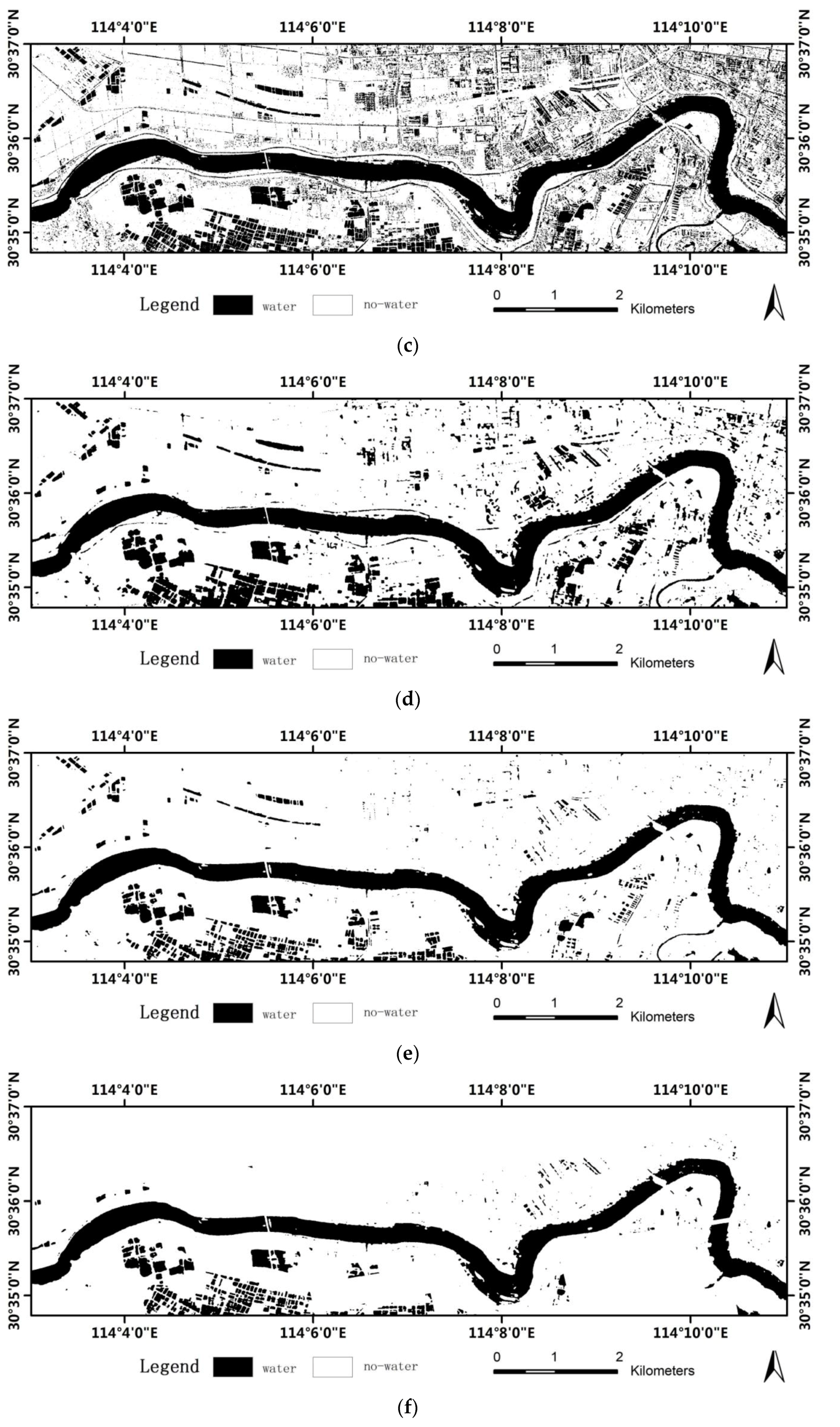
Figure 4 shows the water extraction results for the Huai River. Figure 4a is the SWR generated by the saliency map (see Figure 3d) after post-processing. In general, the actual positions of boundaries within a SAR scene are unknown. Thus, the segmentation quality measures were modified to allow a comparison of the automatic segmentation approaches and manual segmentation, as shown in Figure 4b. Figure 4c–f shows segmentation results by ALG1, ALG2, ALG3 and our method, respectively. Figure 4g shows the post-processing results of the proposed method. The experiment validates that our method (see Figure 4g) performs best in distinguishing water and preventing speckle. Detailed comparisons of accuracy and efficiency are given in Table 1.

4.2. Experiment on TerraSAR-X Imagery

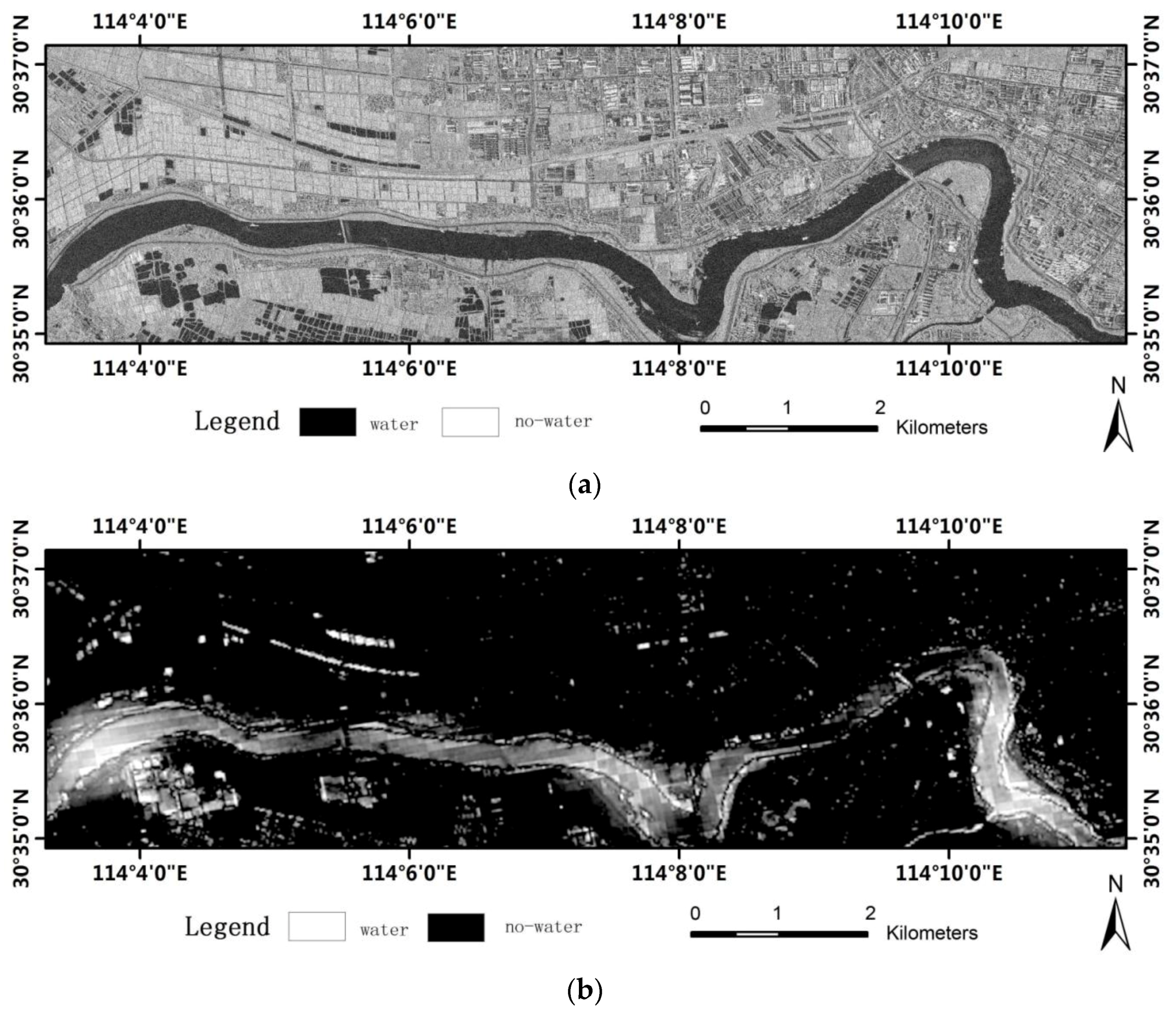
Figure 5 shows a comparative saliency map using a TerraSAR-X image. Figure 5a shows the Hanjiang River in central China, which was acquired by TSX-1 in 2008 in a descending VV polarization mode, with a resolution of 1 m and a size of 7153 × 1948 pixels. After comparing Figure 5b,c, the same conclusions about the model improvements in Radarsat-2 were applicable.
Figure 6 shows the water extraction results for the Hanjiang River. Figure 6a shows the SWR generated using the saliency map (see Figure 5c). Figure 6b is the manual segmentation result. Figure 6c–f show segmentation result by ALG1, ALG2, ALG3 and our method, respectively. Figure 6g shows the post-processing result of the proposed method. The experiment also validates that our method can achieve the best segment result. The speckle noise is very strong in this image, and we can see that there are many very small-scale objects (i.e., “salt and pepper” effects) in Figure 6c,d, and there are many other features misrepresented as water. Figure 6e is much better than the previous methods, however, compared with Figure 6f, there are still some noise effects. Detailed comparisons of accuracy and efficiency are given in Table 1.

4.3. Applications to Large-Area SAR Images

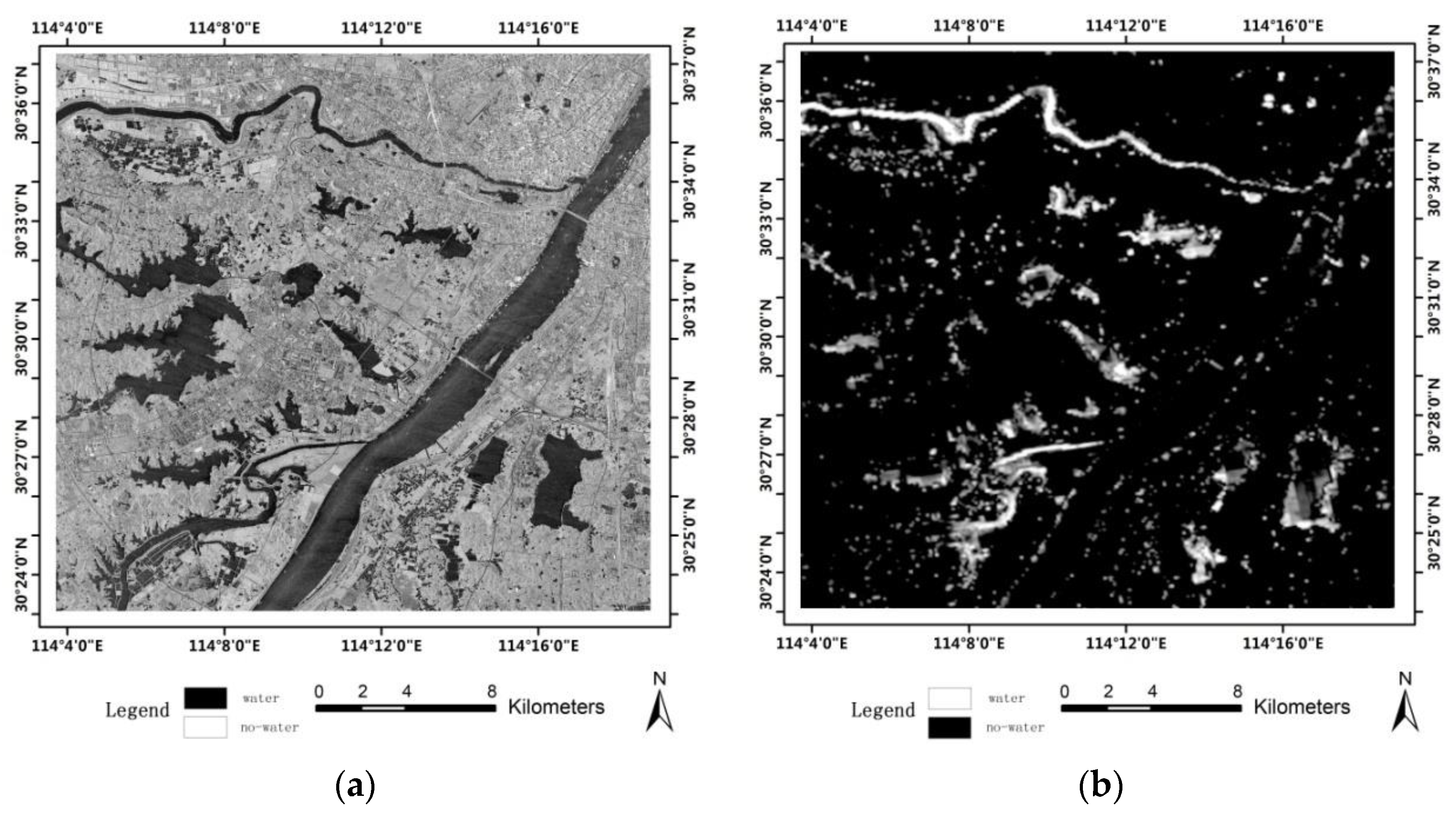
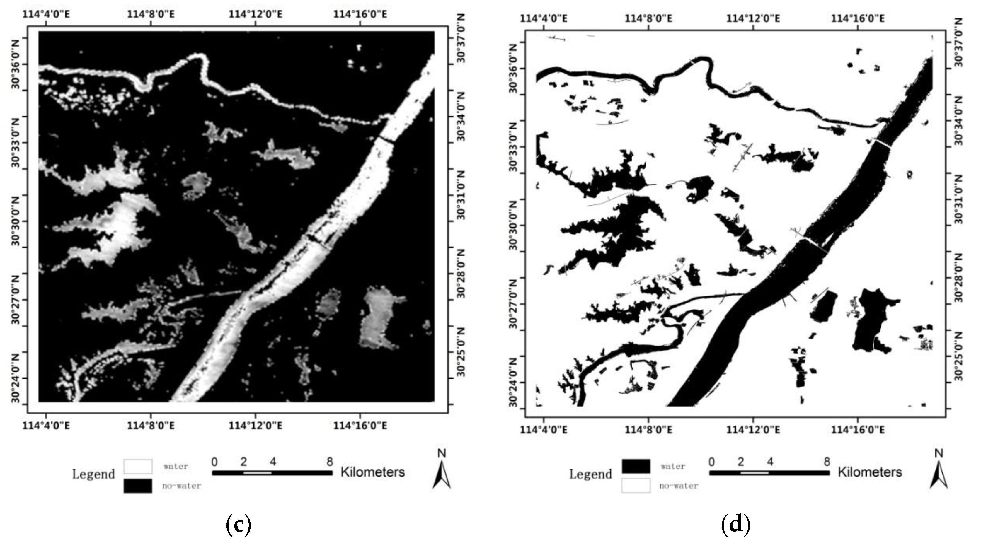
To demonstrate the speed and reliability of our method, we tested the proposed method using real large-area SAR images. The Changjiang River basin, which is one of the main river basins in China, was selected for this experiment. Figure 7 shows the water extraction results for the Changjiang River. Figure 7a shows the original SAR image with an image size of 15540 ×14550 pixels. Figure 7b shows the saliency map generated by Itti model. Figure 7c is the salience map generated using the TW-Itti model and Figure 7d shows the water segmentation result using our method. The time required to generate this image was 1209.463s.

4.4. Accuracy Analysis and Discussion

In order to perform quantitative analysis, overall accuracy (short for OA) and Kappa coefficient are adopted as the accuracy assessment tools in this paper. Assuming that the size of an original SAR image is   M × N , we denote the label image as X ' , whose size is also M × N . Correspondingly, R represents the label image from manual extraction (it also indicates an ideal water extraction) for the same original SAR image. The error image is therefore defined as E = X R .
O A = 1 l M × N × 100 %
where l denotes the number of non-zero pixels in E.
Kappa coefficient can be described as below:
K a p p a = ( M × N ) i r x i i ( x i + x + i ) ( M × N ) 2 ( x i + x + i )
where r is the row numbers of the confusion matrix, x i i is the value of principal diagonal, x i + and x + i are the sum value of row i and column i, respectively.
Table 2 compares the overall accuracy and Kappa coefficient of the above methods.
Based on the qualitative analysis (Experiments 1 and 2) and the quantitative analysis (Table 1), the following conclusions can be reached:
(1)
Compared with the classical Itti model, the improved visual saliency model provides better enhancement of water information and it suppresses other surface features (See Figure 2c,d for Experiment 1and Figure 4b,c for Experiment 2).
(2)
Compared with the state-of-the-art methods (ALG1, ALG2 and ALG3), the method of integration using the multi-scale technique and visual saliency model produced better accuracy.
(3)
In all cases, our method frequently produced superior results and it produced the most accurate results in the shortest time (see Figure 4g for Experiment 1, Figure 6g for Experiment 2 and the bold line in Table 1).
Moreover, in order to better evaluate the performance of the proposed method, the error matrix of the results for ALG1, ALG2, ALG3 and our method were calculated for validation; in this paper, we only take the dataset of Radarsat-2 (Experiment 1) as an example. An error matrix is a very effective way to assess accuracy in that the accuracies of each category are plainly described along with the errors of omission and commission present in the classification. The error matrixes of Experiment 1 are shown in Table 3, Table 4, Table 5 and Table 6.
Overall accuracies for ALG1, ALG2, ALG3 are 79.22% and 92.39%, 91.38%, and the Kappa coefficients are 0.262, 0.53 and 0.511. Individual class accuracies were highly variable, ranging from 20.27% to 99.51%. For our method, overall accuracy is 98.48% and the Kappa coefficient is 0.856. Moreover, individual class accuracies are all very high, above 80%. This proves that our classifier is accurate and robust.

5. Conclusions

The main purpose of this study was to devise a water mapping method that improves accuracy by using a visual attention-based method for multi-scale level sets, particularly in areas with roads, airstrips, radar shadows and paddy fields, which are often major causes of low classification accuracy. Experiments demonstrated that our method significantly improved accuracy in areas where shadow and other dark surfaces were the main sources of classification errors. Our method was aimed at calm water bodies and, therefore, did not consider dynamic water bodies, such as flood water with high wind. In future work, we will focus more on other types of water bodies, looking at, for instance, flood-induced backscatter changes in SAR data [31] and so on.
Although experiments have testified that our method gets satisfactory results, much work remains to be done. The multi-scale analysis framework is a new component in the level set method. In future work, multi-region level sets method can be merged with multi-scale analysis, and, as such, more land features can be considered. Moreover, we will develop our method to be used in full polarized SAR images for acquiring more accurate classification.

Acknowledgments

This work was supported by National Key Fundamental Research Plan of China (973) (No.2012CB719906), major projects of high resolution earth observation system (No. 03-Y20A10-9001-15/16) and National Natural Fund of China (NSFC) (No.41101414).

Author Contributions

Chuan Xu conceived, designed and performed the experiments; Haigang Sui analyzed the data and wrote the paper; Feng Xu provided and analyzed the data.

Conflicts of Interest

The authors declare no conflict of interest.

Abbreviations

The following abbreviations are used in this manuscript:
SARSynthetic Aperture Radar
MLSVSmulti-scale level sets and visual saliency
SWRsuspected water regions
GLCMGray Level Co-occurrence Matrix
LSWLand Surface Water

References

  1. Thomas, H.; Sandro, M.; Andre, T.; Achim, R.; Manfred, B. Extraction of water and flood areas from SAR data. In Proceedings of the 7th European Conference on Synthetic Aperture Radar (EUSAR), Friedrichshafen, Germany, 2–5 June 2008; pp. 1–4.
  2. Lee, J.S.; Iurkevich, I. Segmentation of SAR Image. IEEE Trans. Geosci. Remote Sens. 1989, 27, 981–990. [Google Scholar] [CrossRef]
  3. Sahoo, P.K.; Soltani, S.; Wong, A.K.C. A survey of thresholding techniques. Comput. Vis. Graph. Image Process. 1988, 41, 233–260. [Google Scholar] [CrossRef]
  4. Fiortoft, R.; Lopes, A.; Marthon, P. An optimal multi edge detector for SAR image segmentation. IEEE Trans. Geosci. Remote Sens. 1998, 36, 793–802. [Google Scholar] [CrossRef]
  5. Oliver, C.; Connell, I.M.; White, R.G. Optimum edge detection in SAR. SPIE Satell. Remote Sens. 1995, 2584, 152–163. [Google Scholar] [CrossRef]
  6. Cook, R.; Connell, I.M.; Oliver, C.J. MUM Segmentation for SAR Images. Proc. SPIE 1994, 2316, 92–103. [Google Scholar]
  7. Udupa, J.K.; Samarasekera, S. Fuzzy connectedness and object definition: Theory, algorithms, and applications in image segmentation. Graph. Models Image Process. 1996, 58, 246–261. [Google Scholar] [CrossRef]
  8. Deng, H.; Clausi, D. Unsupervised segmentation of synthetic aperture radar sea ice imagery using a novel Markov random field model. IEEE Trans. Geosci. Remote Sens. 2005, 43, 528–538. [Google Scholar] [CrossRef]
  9. Stéphane, D.; Grégoire, M. Unsupervised multiscale oil slick segmentation from SAR images using a vector HMC model. Pattern Recognit. 2007, 40, 1135–1147. [Google Scholar]
  10. Gan, L.; Wu, Y.; Wang, F.; Zhang, P.; Zhang, Q. Unsupervised SAR image segmentation based on triplet Markov fields with graph cuts. IEEE Geosci. Remote Sens. Lett. 2014, 11, 853–857. [Google Scholar] [CrossRef]
  11. Wang, F.; Wu, Y.; Zhang, Q.; Zhao, W.; Li, M.; Liao, G.S. Unsupervised SAR image segmentation using higher order neighborhood-based triplet Markov fields model. IEEE Trans. Geosci. Remote Sens. 2014, 52, 5193–5205. [Google Scholar] [CrossRef]
  12. Wang, Y.; Li, Y.; Zhao, Q.H. Segmentation of high-resolution SAR image with unknown number of classes based on regular tessellation and RJMCMC algorithm. Int. J. Remote Sens. 2015, 36, 1290–1306. [Google Scholar] [CrossRef]
  13. Huang, B.; Li, H.; Huang, X. A level set method for oil slick segmentation in SAR images. Int. J. Remote Sens. 2005, 26, 1145–1156. [Google Scholar] [CrossRef]
  14. Silveira, M.; Heleno, S. Separation between water and land in SAR images using region-based level sets. IEEE Geosci. Remote Sens. Lett. 2009, 6, 471–475. [Google Scholar] [CrossRef]
  15. Zou, P.F.; Li, Z.; Tian, B.S.; Guo, L.J. A level set method for segmentation of high-resolution polarimetric SAR images using a heterogeneous clutter model. Remote Sens. Lett. 2015, 6, 548–557. [Google Scholar] [CrossRef]
  16. Yin, J.J.; Yang, J. A modified level set approach for segmentation of multiband polarimetric SAR images. IEEE Trans. Geosci. Remote Sens. 2015, 52, 7222–7232. [Google Scholar]
  17. Chan, T.; Vese, L. Active contours without edges. IEEE Trans. Image Process. 2001, 10, 266–277. [Google Scholar] [CrossRef] [PubMed]
  18. Itti, L. Modeling primate visual attention. In Computational Neuroscience: A Comprehensive Approach; Feng, J., Ed.; CRC Press: Boca Raton, FL, USA, 2003; pp. 635–655. [Google Scholar]
  19. Itti, L.; Koch, C.; Niebur, E. Model of saliency-based visual attention for rapid scene analysis. IEEE Trans. Pattern Anal. Mach. Intell. 1998, 20, 1254–1259. [Google Scholar] [CrossRef]
  20. Itti, L.; Gold, C.; Koch, C. Visual attention and target detection in cluttered natural scenes. Opt. Eng. 2001, 40, 1784–1793. [Google Scholar]
  21. Walther, D.; Rutishauser, U.; Koch, C. Selective visual attention enables learning and recognition of multiple objects in cluttered scenes. Comput. Vis. Image Underst. 2005, 100, 41–63. [Google Scholar] [CrossRef]
  22. Li, Z.Q.; Fang, T.; Huo, H. A saliency model based on wavelet transform and visual attention. SCIENCE CHINA Inf. Sci. 2010, 53, 738–751. [Google Scholar] [CrossRef]
  23. Gao, L.N.; Bi, F.K.; Yang, J. Visual attention based model for target detection in large-field images. J. Syst. Eng. Electron. 2011, 22, 150–156. [Google Scholar] [CrossRef]
  24. Li, Z.C.; Itti, L. Saliency and gist features for target detection in satellite images. IEEE Trans. Image Process. 2011, 20, 2017–2029. [Google Scholar] [PubMed]
  25. Sui, H.G.; Xu, C.; Liu, J.Y.; Sun, K.M.; Wen, C.F. A novel multi-scale level set method for SAR image segmentation based on a statistical model. Int. J. Remote Sens. 2012, 33, 5600–5614. [Google Scholar] [CrossRef]
  26. Otsu, N. A threshold selection method from gray-level histogram. IEEE Trans. Syst. Man Cybern. 1979, 9, 62–66. [Google Scholar]
  27. Haralick, R.M.; Shanmugam, K.; Dinstein, I. Textural features for image classification. IEEE Trans. Syst. Man Cybern. 1973, 3, 610–621. [Google Scholar] [CrossRef]
  28. He, L.F.; Chao, Y.Y.; Suzuki, K.J. A run-based two-scan labeling algorithm. IEEE Trans. Image Process. 2008, 17, 749–756. [Google Scholar] [PubMed]
  29. User Guide of eCognition in Chinese. Available online: http://vdisk.weibo.com/s/zt_sYprKIffXK (accessed on 12 October 2015).
  30. Picco, M.; Palacio, G. Unsupervised classification of SAR images using markov random fields and g I 0 Model. IEEE Geosci. Remote Sens. Lett. 2011, 8, 350–353. [Google Scholar] [CrossRef]
  31. Martinis, S.; Twele, A.; Voigt, S. Unsupervised extraction of flood-induced backscatter changes in SAR data using Markov image modeling on irregular graphs. IEEE Trans. Geosci. Remote Sens. 2011, 49, 251–263. [Google Scholar] [CrossRef]
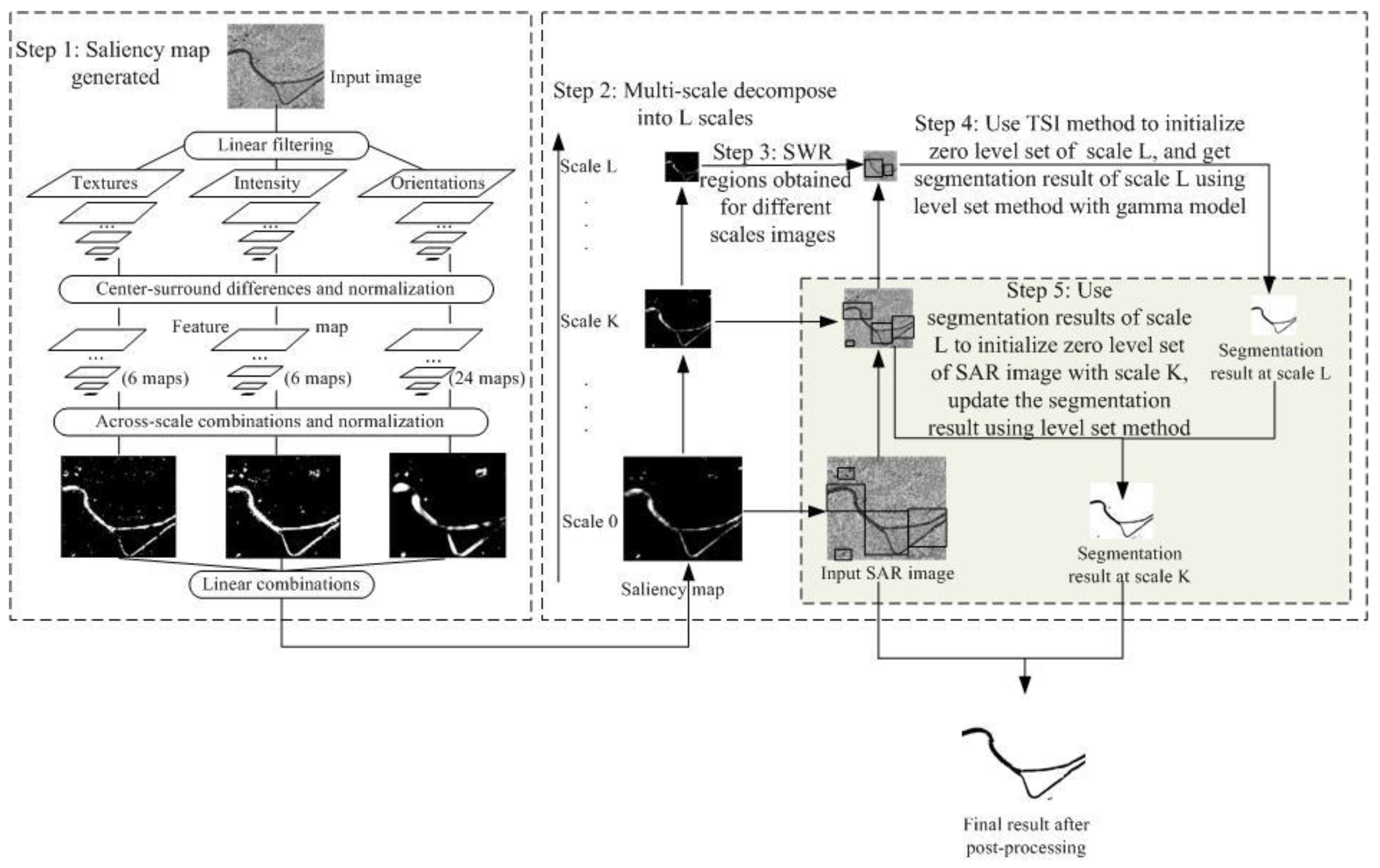
Figure 1. The basic principle of the proposed method. (Step1, saliency map generated from original image; Step 2, Decomposed the saliency map into L scales; Step3, Obtained SWR regions in different scales; Step4, Segmented the water in SWR regions; Step5, refine the segmented result; Step6, post-processing to acquire accurate water body.)
Ijgi 05 00058 g001
Figure 2. The demonstration of the weighting of smoothness within the objects. (a) Single paddy field; (b) connected paddy fields; (c) river; (d) lake.
Ijgi 05 00058 g002
Figure 3. Saliency map comparison (Huai River). (a) Original imagery; (b) Salience map generated by Itti model; (c) Salience map generated by our TW-Itti model; (d) Otsu segmentation result after post-processing of image (c).
Ijgi 05 00058 g003
Figure 4. Segmentation results (Huai River). (a) SWR region generated by Figure 3d; (b) Manual segmentation; (ce) LSW map obtained using ALG1, ALG2 and ALG3,respectively; (f) LSW map obtainedusing proposed method; (g) LSW map obtained after post-processing.
Ijgi 05 00058 g004aIjgi 05 00058 g004b
Figure 5. Saliency map comparison (Hanjiang River). (a) Original imagery; (b) Salience map generated by Itti model; (c) Salience map generated by our model.
Ijgi 05 00058 g005aIjgi 05 00058 g005b
Figure 6. Segmentation results (Hanjiang River). (a) SWR region generated by Figure 4d; (b) Manual segmentation; (ce) LSW map obtained using ALG1, ALG2 and ALG3,respectively; (f) LSW map obtained using our method; (g) LSW map obtained after post-processing.
Ijgi 05 00058 g006aIjgi 05 00058 g006bIjgi 05 00058 g006c
Figure 7. Salience map comparison and segmentation result (Changjiang River). (a) original SAR image; (b) the saliency map generated by Itti model; (c) the saliency map generated by TW-Itti model; (d) LSW map obtained using our method.
Ijgi 05 00058 g007aIjgi 05 00058 g007b
Table 1. Experimental data of different water bodies.
Name of water bodiesHuai RiverHanjiang RiverChangjiang River
SensorRadarsat 2 (VV polarization)TerraSAR-X (VV polarization)TerraSAR-X (VV polarization)
Orbitdescendingascendingascending
ModeUlra-FineSpotlightSpotlight
Date7 December 20099 October 20089 October 2008
Resolution3 m1 m1 m
Image Size (pixels)3024 × 22637153 × 194815540 × 14550
Table 2. Overall Accuracy and Kappa Coefficient Comparison.
MethodOverall Accuracy (%)Kappa Coefficient
Experiment on Radarsat-2 imagery
ALG179.220.262
ALG292.390.530
ALG391.380.511
Proposed Method98.480.856
Experiment on TerraSAR-X imagery
ALG181.800.434
ALG288.710.577
ALG394.170.731
Proposed Method98.420.913
Table 3. Error matrix of the ALG1 classified image (Dataset 1).
ClassReference Data
WaterNon-WaterTotal
Water35152313830031734526
Non-water3878950699975108786
Total39031264530006843312
Overall accuracy = 79.22% Kappa coefficient = 0.262
Producer accuracy
Water=351523/390312=90.06%
Non-water=5069997/6453000=78.57%
User accuracy
Water=351523/1734526=20.27%
Non-water=5069997/5108786=99.24%
Table 4. Error matrix of the ALG2 classified image (Dataset 1).
ClassReference Data
WaterNon-WaterTotal
Water340153470767810920
Non-water5015959822336032392
Total39031264530006843312
Overall accuracy = 92.39% Kappa coefficient = 0.53
Producer accuracy
Water=340153/390312=87.15%
Non-water=5982233/6453000=92.7%
User accuracy
Water=340153/810920=41.95%
Non-water=5982233/6032392=99.17%
Table 5. Error matrix of the ALG3 classified image (Dataset 1).
ClassReference Data
WaterNon-WaterTotal
Water361014560267921281
Non-water2929858927335922031
Total39031264530006843312
Overall accuracy = 91.38% Kappa coefficient = 0.511
Producer accuracy
Water=361014/390312=92.49%
Non-water=5892733/6453000=91.32%
User accuracy
Water=361014/921281=39.19%
Non-water=5892733/5922031=99.51%
Table 6. Error matrix of the proposed method classified image (Dataset 1).
ClassReference Data
WaterNon-WaterTotal
Water32967143053390312
Non-water6064164099476453000
Total39031264530006843312
Overall accuracy = 98.48% Kappa coefficient = 0.856
Producer accuracy
Water=329671/390312=84.46%
Non-water=5069997/6453000=99.33%
User accuracy
Water=329671/390312=88.45%
Non-water=6409947/6453000=99.06%