A Hybrid Method for Interpolating Missing Data in Heterogeneous Spatio-Temporal Datasets

Abstract

Space-time interpolation is widely used to estimate missing or unobserved values in a dataset integrating both spatial and temporal records. Although space-time interpolation plays a key role in space-time modeling, existing methods were mainly developed for space-time processes that exhibit stationarity in space and time. It is still challenging to model heterogeneity of space-time data in the interpolation model. To overcome this limitation, in this study, a novel space-time interpolation method considering both spatial and temporal heterogeneity is developed for estimating missing data in space-time datasets. The interpolation operation is first implemented in spatial and temporal dimensions. Heterogeneous covariance functions are constructed to obtain the best linear unbiased estimates in spatial and temporal dimensions. Spatial and temporal correlations are then considered to combine the interpolation results in spatial and temporal dimensions to estimate the missing data. The proposed method is tested on annual average temperature and precipitation data in China (1984–2009). Experimental results show that, for these datasets, the proposed method outperforms three state-of-the-art methods—e.g., spatio-temporal kriging, spatio-temporal inverse distance weighting, and point estimation model of biased hospitals-based area disease estimation methods.

1. Introduction

Evolving patterns of geographical phenomena are usually modeled as spatio-temporal processes depicted by space-time data. Nearly all instrumental space-time data are influenced by missing data [1,2]. Before data analysis, missing data must be well handled. To treat missing data, two common approaches are available. One is to exclude periods with missing values from data analysis, and the other is to ignore the missing data based on the tacit assumption that the data represent one continuous series [3,4]. However, these approaches may disregard useful information and bias the analysis results [2]. To overcome these limitations, a number of interpolation methods have been proposed to estimate missing observations in space-time data. Most of these methods assume that the interpolation of space-time data can be reducible to a sequence of spatial interpolations [5]. However, applying spatial interpolation methods to space-time data usually leads to the loss of valuable information in the temporal dimension [6]. On that account, space-time interpolation methods that consider both spatial and temporal dimensions have been paid more attention and have been widely used in geoscience [7,8,9].

Currently, a series of space-time interpolation methods have been developed based on spatial interpolation methods—i.e., space-time inverse distance weighting methods, space-time kriging methods, and regression-based methods [10,11,12]. Although space-time interpolation plays a key role in space-time modeling, existing methods mainly assume that space-time processes exhibit stationarity in space and time. However, the second order stationarity (mean and variance of a process are all constants), even the first order stationarity (mean of a process is constant) is usually not satisfied in practice [13,14,15]. Owing to the heterogeneity of space-time data, the accuracy of the interpolation results obtained by existing methods is still unsatisfactory. Therefore, a space-time interpolation method considering both spatial and temporal heterogeneity is developed for treating missing data. First, heterogeneous covariance functions are constructed for both spatial and temporal dimensions, and the best linear unbiased estimates in spatial and temporal dimensions are obtained. Spatial and temporal correlations are then considered to combine the interpolation results in spatial and temporal dimensions to estimate the missing data. The effectiveness and advantage of the proposed method are empirically evaluated in terms of an annual temperature and precipitation dataset spanning 1984 to 2009 in China.

The remainder of this paper is organized as follows. In Section 2, the related works of spatio-temporal interpolation are reviewed, and a new strategy is developed. In Section 3, the proposed space-time interpolation method is represented. In Section 4, two experimental datasets are selected to demonstrate the validity of the proposed method. In Section 5, conclusions are drawn at the end of the paper.

2. Spatio-Temporal Interpolation: Related Work and Our Strategy

Existing methods for estimating missing data can be roughly divided into three types: regression based, inverse distance weighting (IDW), and kriging methods. In the following, details of these methods will be reviewed.

2.1. Related Work

Regression-based methods construct a regression function to estimate missing data by integrating surrounding station records and relevant information as explanatory variables. The conventional methods—i.e., simple and multiple regression methods—do not consider spatial autocorrelation. To overcome this limitation, some spatial regression models have been developed—e.g., spatial lag and spatial error models [16]. However, spatial heterogeneity (first-order or second-order non-stationarity) and temporal dimension are not considered by these spatial regression models. Although geographically weighted regression (GWR) and spatio-temporal geographically weighted regression (STGWR) are able to construct a regression function for each location [17,18,19], the regression function between missing data and explanatory variables cannot be constructed. Therefore, GWR and STGWR are unsuitable for estimating missing data. A spatial regression test (SRT) estimates the missing data in the station of interest by using the neighboring stations [20,21]. For each neighboring station, a regression estimate (x_i = a_i + b_iy_i) is calculated. The values of missing data are calculated as weighted averages of the estimates. Although SRT has the potential to consider spatial heterogeneity, temporal heterogeneity cannot be considered, and there is no objective function for the best linear unbiased estimates [5].

The inverse distance weighting (IDW) methods are also widely used for estimating missing data. The IDW methods weight the values at neighboring stations according to the inverse of the distances separating the locations. The IDW methods simply assume that neighboring stations are related to the station of interest by their proximity to the station of interest. Some variants of IDW were also developed by using different weighting schemes [22,23]. Some studies attempted to integrate time and space dimensions in IDW, and spatio-temporal IDW (STIDW) methods were proposed [24]. STIDW first defined a three-dimensional space-time distance and then applied the space-time distance in IDW to estimate the missing values. Although the IDW and STIDW methods are easy to implement, they have difficulty obtaining nonbiased estimates.

Kriging and its variants have also been applied to estimate missing data [25,26,27]. These methods are able to obtain unbiased predictions with minimal variance. To consider the temporal dimension, spatio-temporal kriging methods have also been developed [28]. The derivation of the spatio-temporal covariance function plays a key role in spatio-temporal kriging methods. There are two kinds of spatio-temporal covariance functions: separable and non-separable models [25,29]. In the separable model, the spatio-temporal covariance function is treated as either a sum or product of separate spatial and temporal covariance functions [30]. In the non-separable model, the spatio-temporal covariance function is treated as a non-linear, multiplicative version of the spatial and temporal covariance functions [6,10,31,32,33]. However, spatio-temporal kriging methods assume that a space-time process has a constant mean and variance (i.e., second order stationarity) in space and time [13,15]. To overcome this limitation, a point estimation model of biased hospitals-based area disease estimation, named P-Bshade, is developed [5,34]. P-Bshade directly calculates the covariance of the historical observation data to determine the weighting coefficients of surrounding observation stations. The P-Bshade method is mainly designed for spatial interpolation; thus, the temporal dimension is not considered to estimate the missing data.

2.2. A Critical Analysis of Existing Work and Our Strategy

Based on the above analysis, the performance of existing methods can be summarized as follows:

(a)

Currently, missing data in a spatio-temporal dataset are mainly estimated by using spatial interpolation methods—e.g., spatial regression models, SRT, IDW, kriging, and P-Bshade. The neglect of time dimension will lead to the loss of valuable information in the estimation of missing data; and

(b)

Although a few spatio-temporal interpolation methods are currently available for estimating missing data—e.g., STIDW and spatio-temporal kriging—the heterogeneity (i.e., second-order non-stationarity) of spatio-temporal data should be further considered [35].

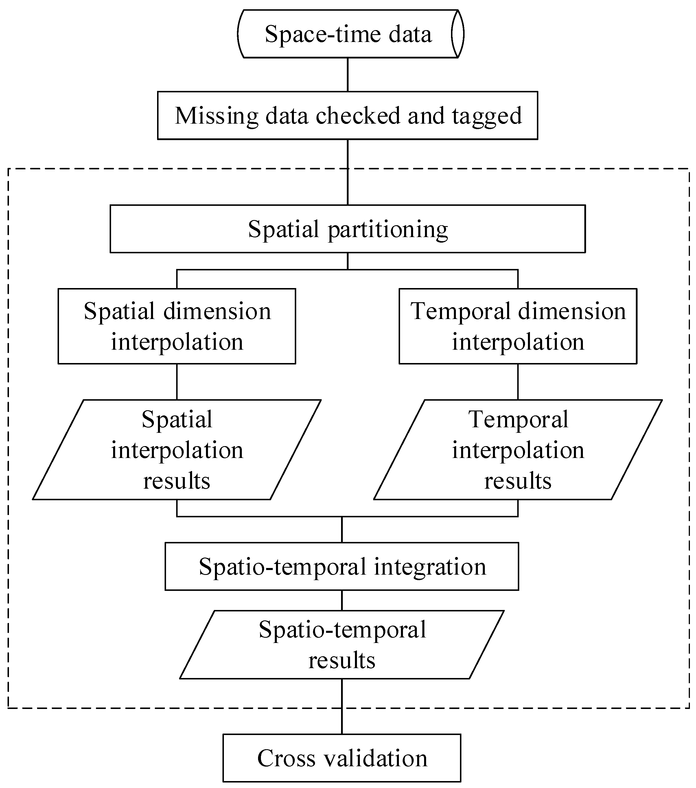
On that account, a new strategy should be developed. In this study, we assume that both spatial and temporal distributions of the spatio-temporal data are non-homogeneous (i.e., second-order non-stationarity). Motivated by the separable spatio-temporal covariance function, the space-time variable of interest is treated as a sum of independent spatial and temporal non-stationarity components. Heterogeneous covariance functions are then constructed for both spatial and temporal dimensions, and objective functions are maximized to obtain the best linear unbiased estimates in spatial and temporal dimensions. Finally, spatial and temporal correlations are considered to combine the interpolation results in spatial and temporal dimensions to estimate the missing data. The performance of the space-time interpolation operation will be evaluated by using cross-validation. In Figure 1, the strategy proposed in this study is shown. In the following, the spatio-temporal interpolation method will be represented.

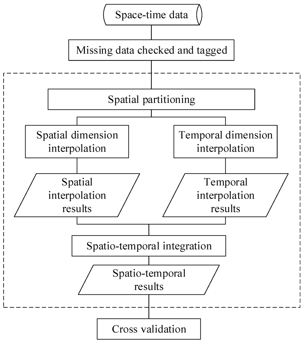
Figure 1. The flowchart of this method.

3. Hybrid Interpolation Method for Heterogeneous Spatio-Temporal Data

Based on the strategy introduced in Section 2.2, spatial and temporal interpolations will be performed. A weighted sum of observations is used to obtain unbiased and minimal error variance estimates of missing data. To calculate the weights, heterogeneous covariance functions are constructed for spatial and temporal dimensions.

3.1. Heterogeneous Covariance Functions for Handling Space-Time Heterogeneity

As elaborated in Figure 1, we first check the space-time data to tag the unsampled space-time position. Then, a hierarchical clustering method—REDCAP (regionalization with dynamically constrained agglomerative clustering and partitioning) was employed to partition the study area into homogenous spatial regions based on the average observations at each station [36,37]. The REDCAP method consists of two steps: spatial contiguity constrained hierarchical clustering and spatially-contiguous tree partitioning. In the first step, a hierarchical clustering method is first used to construct a spatially contiguous tree. In this study, average linkage is selected as the hierarchical clustering method. The spatially-contiguous tree is then partitioned into a number of sub-trees by minimizing an objective function. The objective function is defined as the total heterogeneity of all regions, represented as:

$$H_k={\displaystyle \sum _{i=1}^k{\displaystyle \sum _{j=1}^{n_i}{(x_{ij}-{\overline{x}}_i)}^2}}$$

(1)

where k is the number of regions, n_i is the number of objects in ith region, x_ij is the attribute value of the jth object in ith region, and ${\overline{x}}_i$ is the mean attribute value of the ith region.

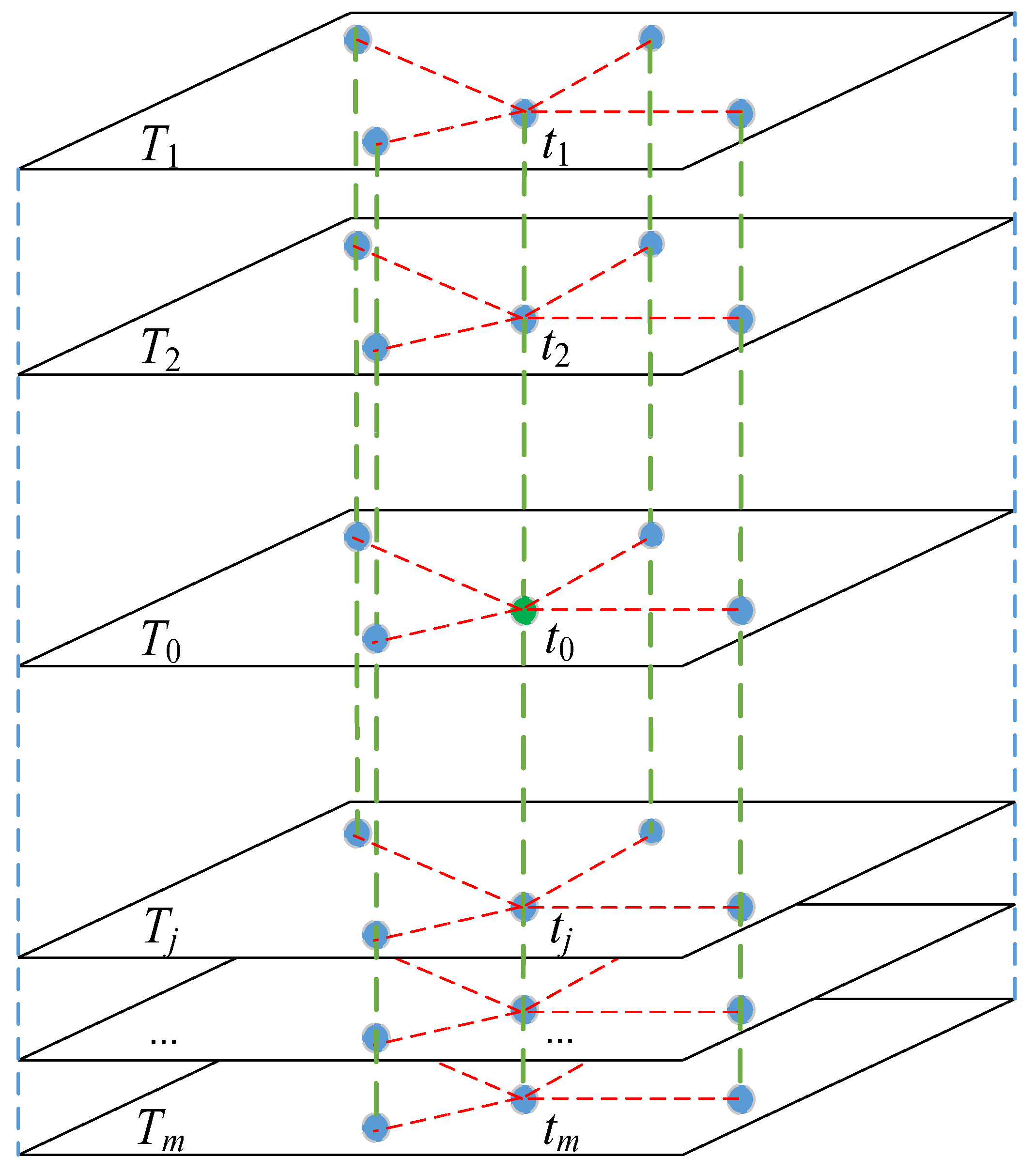
After the homogenous sub-regions are obtained, the missing values are interpolated in the temporal dimension. The m temporal neighbors of the missing value will be generated at first. As shown in Figure 2, let t₀ be a missing value in region k_i at the time layer T₀, m most correlated time layers of T₀ are determined based on region k_i. In detail, the pair-wise objects for calculating the correlation between time layer T₀ and T_j is identified as observed records in k_i with same location. Then, at each correlated time layer of T₀, the observed record with the same location of t₀ is identified as a temporal neighbor of t₀. For example, in Figure 2, if {T₁, T₂, …, T_m} are the m most correlated time layers of T₀, the m temporal neighbors of t₀ are formed by {t₁, t₂, …, t_m}. In the temporal dimension, the estimated value (${\widehat{t}}_0$) of missing record t₀ is calculated according to Equation (2):

$${\widehat{t}}_0={\sum }_{j=1}^m{\phi }_j{t}_j$$

(2)

where t_j denotes the jth temporal neighbor of missing record t₀ in temporal dimension, and φ_j denotes the corresponding contribution weight of t_j. The missing records can be calculated by the other records of missing observation stations using Equation (2). To ensure that ${\widehat{t}}_0$ is the unbiased estimate for the missing records, the following relationship should be satisfied:

$$E(t_0)=E({\widehat{t}}_0)$$

(3)

where t₀ represents the real value of missing value, E(t₀) represents the statistical expectation of t₀ in temporal dimension. Substituting Equation (2) into Equation (3), Equation (4) can be rewritten as:

$$E(t_0)=E({\sum }_{j=1}^m{\phi }_j{t}_j)$$

(4)

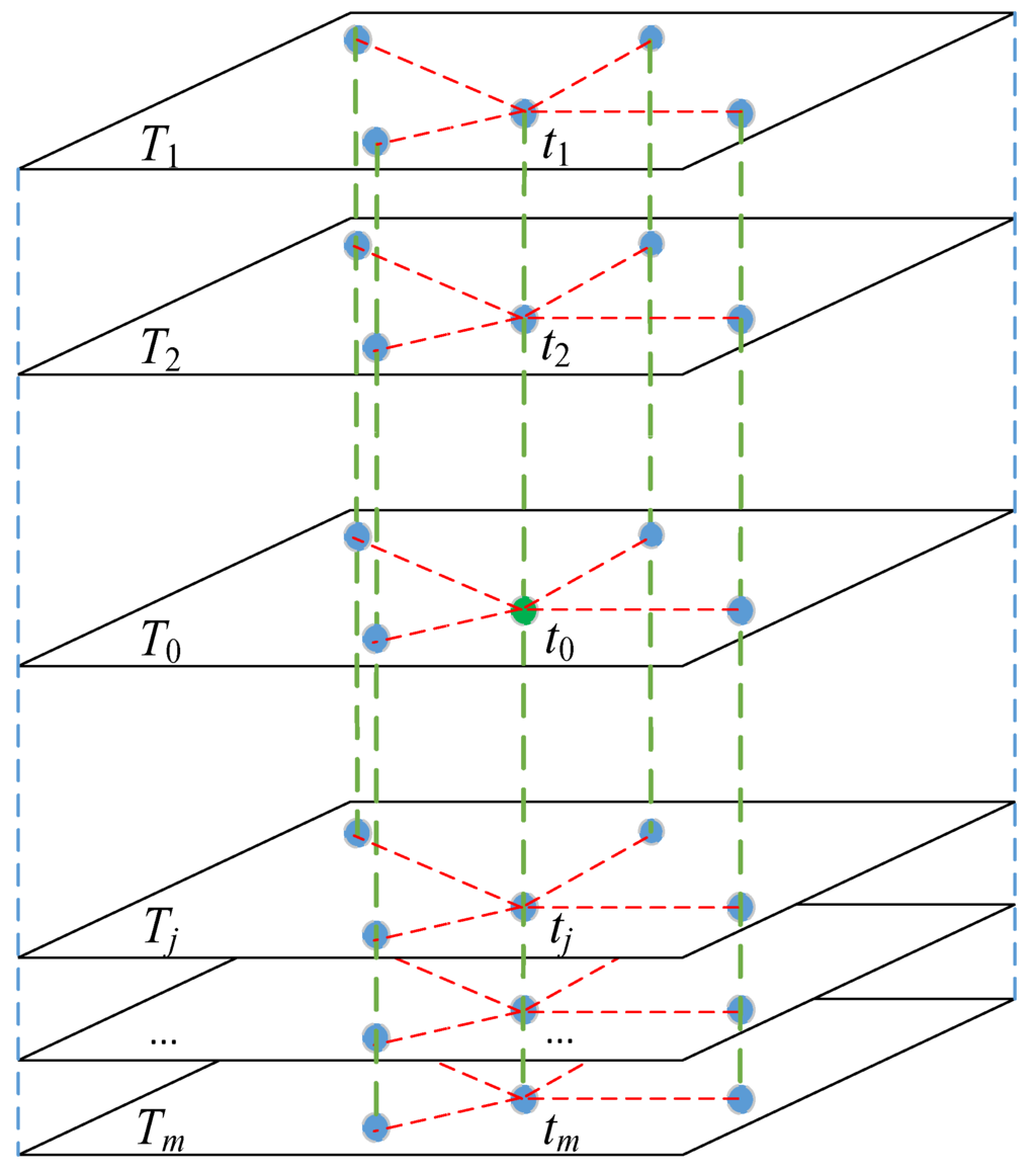
Figure 2. Interpolation in temporal dimension (blue dots represent observed records; red dotted lines are used to represent the spatial relationships).

In view of temporal heterogeneity, we introduce a parameter of ratio a_j calculated according to Equation (5). The parameter a_j is used to represent the heterogeneity between two time layers:

$$a_j=E(t_j)/E(t_0)$$

(5)

In Equation (5), if E(t_j) = 0 or E(t₀) = 0, a small positive constant (e.g., 0.0001) is added to E(t_j) or E(t₀). Combining Equations (4) and (5), the unbiased estimates of φ_j can be determined by minimizing the variance $E{\left({\widehat{t}}_0-t_0\right)}^2$according to Equation (6).

$$\{\begin{array}{c}{\displaystyle \underset{\phi }{\text{argmin}}}{\sigma }_{{\widehat{t}}_0}^2={\displaystyle \underset{\phi }{\text{argmin}}}E{({\widehat{t}}_0-t_0)}^2\\ s.t.{\sum }_{j=1}^m{\phi }_j{a}_j=1\end{array}$$

(6)

With the restrictions of Equation (6), the minimized estimation error variance in temporal dimension can be represented as follows:

$${\sigma }_{{\widehat{t}}_0}^2={\sigma }^2+{\sum }_{j=1}^m{\sum }_{g=1}^m{\phi }_j{\phi }_{g}C(t_j,t_g)-2{\sum }_{j=1}^m{\phi }_{j}C(t_j,t_0)+2\upsilon ({\sum }_{j=1}^m{\phi }_j{a}_j-1)$$

(7)

where υ is a Lagrange multiplier. Furthermore, we can calculate the weight φ_j based on Equation (7) and obtain the estimates of unsampled data based on Equation (2).

After the interpolation in the temporal dimension is finished, the interpolation in the spatial dimension will be implemented similar to that in the temporal dimension. In each homogenous sub-region, the largest correlated n stations are selected to interpolate the missing value in a station, and the correlation between two stations is calculated based on the observed time series. The estimated value of missing value ${\widehat{y}}_0$ is calculated according to Equation (8):

$${\widehat{y}}_0={\sum }_{i=1}^n{w}_i{y}_i$$

(8)

where y_i denotes the observed record in station i at the same time layer of the missing value y₀, w_i denotes the corresponding contribution weight of y_i, and ${\widehat{y}}_0$ is defined as an unbiased estimate for the missing value y₀. Similarly to Equations (6) and (7), the minimized estimation error variance in spatial dimension can be represented as follows:

$${\sigma }_{{\widehat{y}}_0}^2={\sigma }^2+{\displaystyle {\sum }_{i=1}^n{\displaystyle {\sum }_{k=1}^n{w}_i}}{w}_{k}C(y_i,y_k)-2{\displaystyle {\sum }_{i=1}^n{w}_i}C(y_i,y_0)+2\mu ({\displaystyle {\sum }_{i=1}^n{w}_i}{b}_i-1)$$

(9)

where μ is a Lagrange multiplier. Furthermore, we can calculate the weight w_i based on Equation (9) and obtain the estimates of the missing values based on Equation (8).

3.2. Estimating Spatio-Temporal Missing Data by Combining Both Spatial and Temporal Information

To calculate the missing value t₀ in region k_i at time layer T₀ in temporal dimension, m most correlated time layers and m temporal neighbors are first generated based on the method introduced in Section 3.1. In Equation (7), minimizing ${\sigma }_{{\widehat{t}}_0}^2$ with respect to weights φ_j (j = 1, 2, ..., m) and taking the partial derivative with respect to φ_j, Equation (7) can be expanded into a matrix equation as follows:

$$\left[\begin{array}{cccc}C(t_1,t_1)& \cdots & C(t_1,t_m)& a_1\\ ⋮& C(t_j,t_{j^{\prime }})& ⋮& ⋮\\ C(t_m,t_1)& \cdots & C(t_m,t_m)& a_m\\ a_1& \cdots & a_m& 0\end{array}\right]\left[\begin{array}{l}{\phi }_1\\ ⋮\\ {\phi }_m\\ \upsilon \end{array}\right]=\left[\begin{array}{c}C(t_1,t_0)\\ ⋮\\ C(t_m,t_0)\\ 1\end{array}\right]$$

(10)

where υ is also the Lagrange multiplier, $C\left(t_j,t_{j^{‘}}\right)$ is the covariance between the jth time layer and the j’th time layer calculated based on the records in region k_i, and pair-wise objects for calculating $C\left(t_j,t_{j^{\prime }}\right)$ are identified as records in k_i with the same location. $C\left(t_j,t_0\right)$ is the covariance between the jth time layer and time layer T₀ with missing values. The calculation of $C\left(t_j,t_0\right)$ is similar to that of $C\left(t_j,t_{j^{\prime }}\right)$; however, only observed records are involved to calculated the covariance. a_j denotes a ratio between time layer T_j and time layer T₀ with missing values (calculated by Equation (5)).

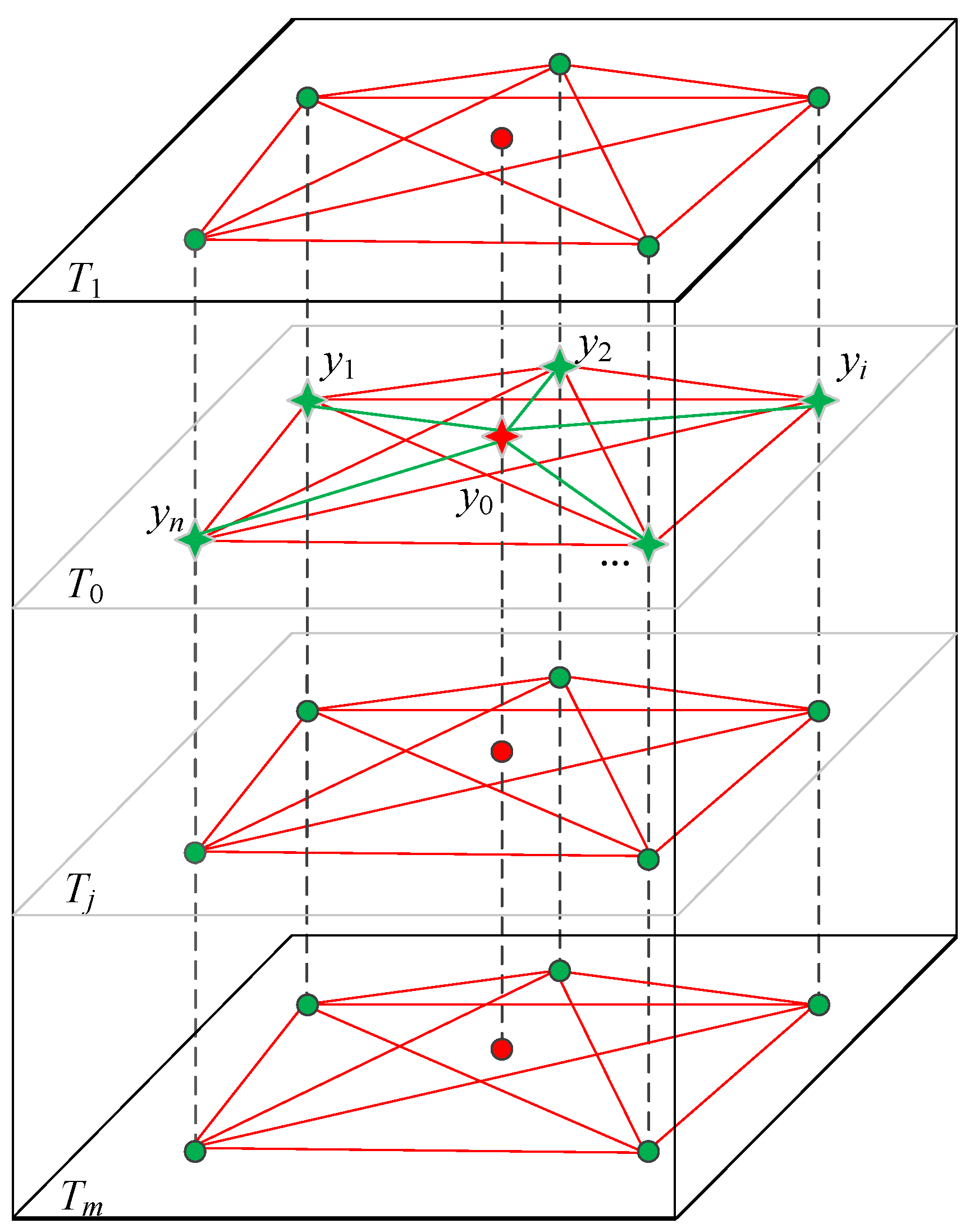
Then, to calculate the missing value y₀ in the region k_i at time layer T₀ in the spatial dimension, the largest correlated n stations are first selected based on the method introduced in Section 3.1. As shown in Figure 3, the red star is the station with the missing value y₀. The green stars represent the largest correlated n stations of the station with the missing value (n = 5). The red dots represent the temporal neighbors of the missing value, and the green dots represent other observed records. In Equation (9), minimizing ${\sigma }_{{\widehat{y}}_0}^2$ with respect to weights w_i (i = 1, 2, ..., n) and taking the partial derivative with respect to w_i, Equation (9) can be expanded into a matrix equation as Equation (11):

$$\left[\begin{array}{cccc}C(y_1,y_1)& \cdots & C(y_1,y_n)& b_1\\ ⋮& C(y_i,y_{i^{\prime }})& ⋮& ⋮\\ C(y_n,y_1)& \cdots & C(y_n,y_n)& b_n\\ b_1& \cdots & b_n& 0\end{array}\right]\left[\begin{array}{l}{w}_1\\ ⋮\\ w_n\\ \mu \end{array}\right]=\left[\begin{array}{c}C(y_1,y_0)\\ ⋮\\ C(y_n,y_0)\\ 1\end{array}\right]$$

(11)

where μ denotes the Lagrange multiplier, $C\left(y_i,y_{i^{\prime }}\right)$ on the left-hand side of Equation (11) is the covariance between the station i and the station i’, calculated based on the time series of these two stations. $C\left(y_i,y_0\right)$ on the right-hand side of Equation (11) is the covariance between the station i and station with missing value, calculated based on the observed time series of these two stations. b_i denotes a ratio between station i and the station with the missing value, calculated by E(y_i)/E(y₀), where E(y_i) represents mean value of the time series at station i. The matrix consisting of the contribution weights w_i can be calculated by Equation (11).

Figure 3. Interpolation in the spatial dimension.

Finally, the estimated values in the spatial and temporal dimensions should be integrated to obtain the overall estimated value Y_ij of the missing value. There are mainly two kinds of space-time geostatistical models, i.e., the separable model and non-separable model [29]. The separable model is easy to implement; however, the space-time interaction may be not well considered. Although the non-separable model is able to consider the space-time interaction, in theory, the construction of the non- separable model for the non-stationarity space-time variable is very difficult [30]. In this study, spatial and temporal dimensions are both considered to calculate the interpolation results in spatial or temporal dimensions, e.g., the solution of Equations (10) and (11). Thus, we think that, to some degree, space-time interaction is considered in spatial and temporal dimension interpolation. Therefore, the overall estimated value Y_ij is defined as a weighted sum of estimated values in spatial and temporal dimensions, represented as follows:

$$Y_{ij}=A{\widehat{y}}_0+B{\widehat{t}}_0$$

(12)

where i is the station number, j is the time series number, A is the weight in spatial dimension, and B is that in temporal dimension (A + B = 1). In this study, the weights in spatial and temporal dimensions are calculated according to the correlation coefficient, represented as follows:

$$\frac{A}{B}=\frac{{\displaystyle \sum _{i=1}^{n}R\left(y_{\mathrm{i}},y_0\right)}}{n}/\frac{{\displaystyle \sum _{j=1}^{m}R\left(t_j,t_0\right)}}{m}, A+B=1$$

(13)

where n represents the number of spatial neighbors and m represents the number of temporal neighbors. R(y_i, y₀) represents the correlation between the missing value and its spatial neighbors, measured by the correlation coefficient between the observed time series of station i and that of the station with missing value y₀. R(t_j, t₀) represents the correlation between the missing value and its temporal neighbors, measured by the correlation coefficient between time layer T₀ and T_j calculated based on region k_i (t_j∈k_i, t₀ ∈k_i). From Equation (13), it can be found that if the missing value is more correlated with its spatial neighbors (temporal neighbors); thus, the weight in the spatial dimension (temporal dimension) will be heavy. After the weights in the spatial and temporal dimensions are calculated by solving Equation (13), the final estimation results of missing data can be obtained by Equation (12).

4. Experiments and Results Analysis

The proposed interpolation method is implemented in MATLAB 2014b. The average annual temperature and precipitation data from 554 meteorological stations during the period from 1984 to 2009 is selected to validate the proposed interpolation method. These experimental data are provided by the China National Meteorological Information Center (CNMIC). In these datasets, some temperature and precipitation records are missing. In Figure 4, the numbers of missing records in different years are shown. One can find that the number of missing data decreased sharply around 1995, gradually reaching a stable level around that year. The maximal number of missing records is 30 (in the year 1984), and the minimal number of missing records is eight (in the year 2001 and 2002).

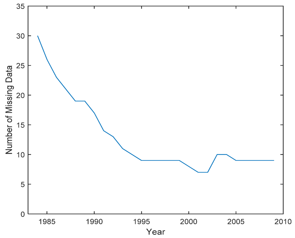
Figure 4. The number of missing records from 1984 to 2009.

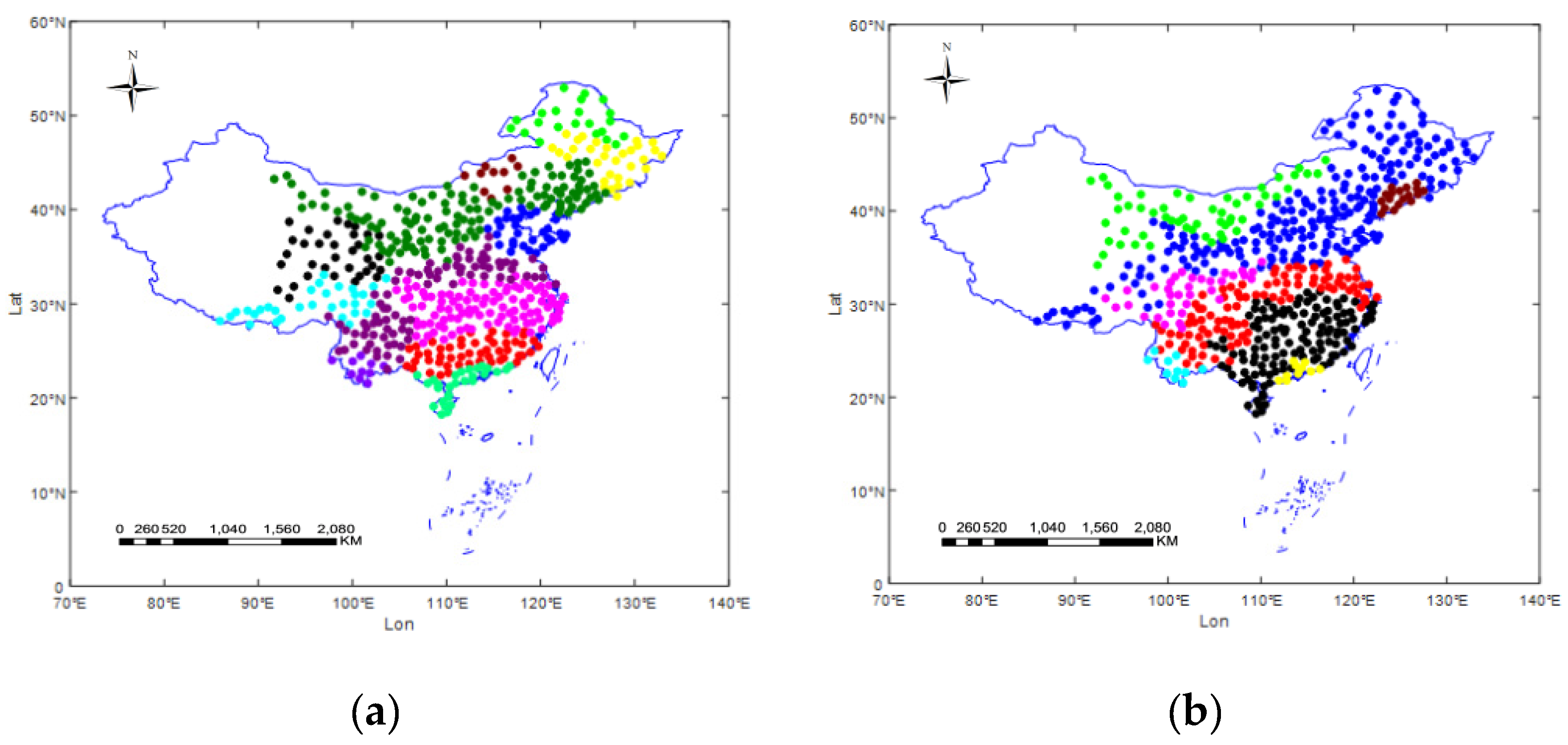
As illustrated in Figure 5, the whole study area including 554 observation stations are partitioned into different homogenous sub-regions. Dots of identical color belong to the same sub-region. The number of sub-regions is determined by REDCAP, which is set as 12 for temperature observations and eight for precipitation observations. The number of clusters is determined based on the prior knowledge (e.g., climate zones in China) and the clustering validity index (L-method). The number of neighboring stations is determined based on the existing study and clustering results. Based on experiments, Xu et al. [5] suggested that the number of neighboring stations can be set from 5–15. It is also known that stations are similar to one another in the same cluster and are dissimilar to stations in different stations. Thus, the number of neighboring stations cannot be larger than the size of the smallest cluster. On the basis of these principles, the number of spatial neighbors n is set to 10. Hubbard et al. [20,21] suggested that the number of temporal neighbors can be set to about half of the research period. In this study, the research period is 26, therefore the number of temporal neighbors m is also set to 10.

Figure 5. Homogenous sub-regions of (a) temperature and (b) precipitation.

Particularly, the interpolation results of other three widely used methods (spatio-temporal kriging with product-sum covariance method [6], denoted as STKriging; spatio-temporal inverse distance weighting, denoted as STIDW; and point estimation model of biased hospital-based area disease estimation, denoted as P-Bshade), and this proposed method, i.e., space-time heterogeneous covariance method (denoted as STHC) are compared to evaluate the accuracy. To implement the STKriging, a data pre-process operation is first implemented to guarantee second-order stationarity. In the temporal dimension, no obvious trend or periodicity is found. In the spatial dimension, the trend is estimated in each spatial location by using a moving window, and a local trend estimation procedure with an optimum window size proposed by Pelletier, et al. [38] is employed to estimate the trend. In each window, the polynomial of order one is used to model the trend. In addition, STKriging and STIDW are also performed in each sub-region obtained by the clustering method, denoted as STKriging-Partition and STIDW-Partition. To assess the performance of different interpolation methods, annual station records in China from 1984 to 2009 were estimated by leave-one-out cross-validation [39]. Each observed record is first removed, and then the estimated value is compared with the true observed value. Three indicators, i.e., mean absolute error (MAE), root mean square error (RMSE), and coefficient of determination (r²), are calculated to evaluate the accuracy of the interpolation results. The statistical results are shown in Table 1.

Table 1. Experimental results of different interpolation methods.

Methods	TEM				PRE
	MAE (°C)	RMSE (°C)	r2	Residual Autocorrelation	MAE (mm)	RMSE (mm)	r2	Residual Autocorrelation
STKriging	1.43	2.20	0.990	0.25	19.93	38.56	0.864	0.77
STIDW	2.08	2.76	0.926	0.28	30.31	52.27	0.659	0.80
STKriging-Partition	1.13	1.45	0.994	0.23	19.13	33.39	0.879	0.72
STIDW-Partition	1.63	2.15	0.990	0.27	27.07	47.37	0.709	0.76
P-Bshade	0.41	0.50	0.996	0.25	18.69	35.20	0.870	0.68
STHC	0.23	0.33	0.998	0.20	17.26	31.64	0.909	0.63

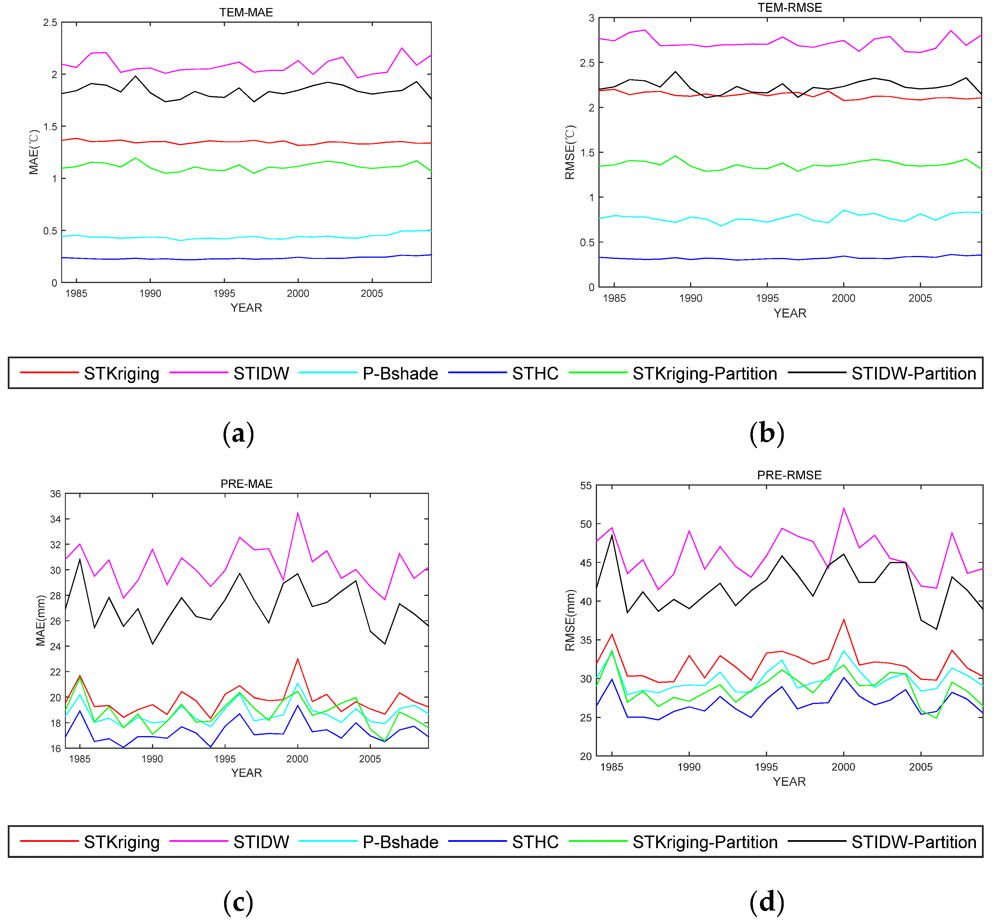
As listed in Table 1, it can be found that the accuracy of our method is obviously higher than that of the other methods. For temperature and precipitation data, the MAE and RMSE values of our method are significantly lower than those of STKriging, STIDW, STKriging-Partition, and STIDW-Partition methods, showing great improvement in interpolation accuracies. The interpolation accuracy of our method is also higher than that of P-Bshade method, even though the improvement is less remarkable. The values of MAE and RMSE per year are shown in Figure 6. For the temperature data, the MAE error of the proposed method is significantly lower than other methods over the years, as well as RMSE. For the precipitation data, it also can be found that the proposed method has the least MAE and RMSE error. However, two serious errors appeared in the years 1985 and 2000.

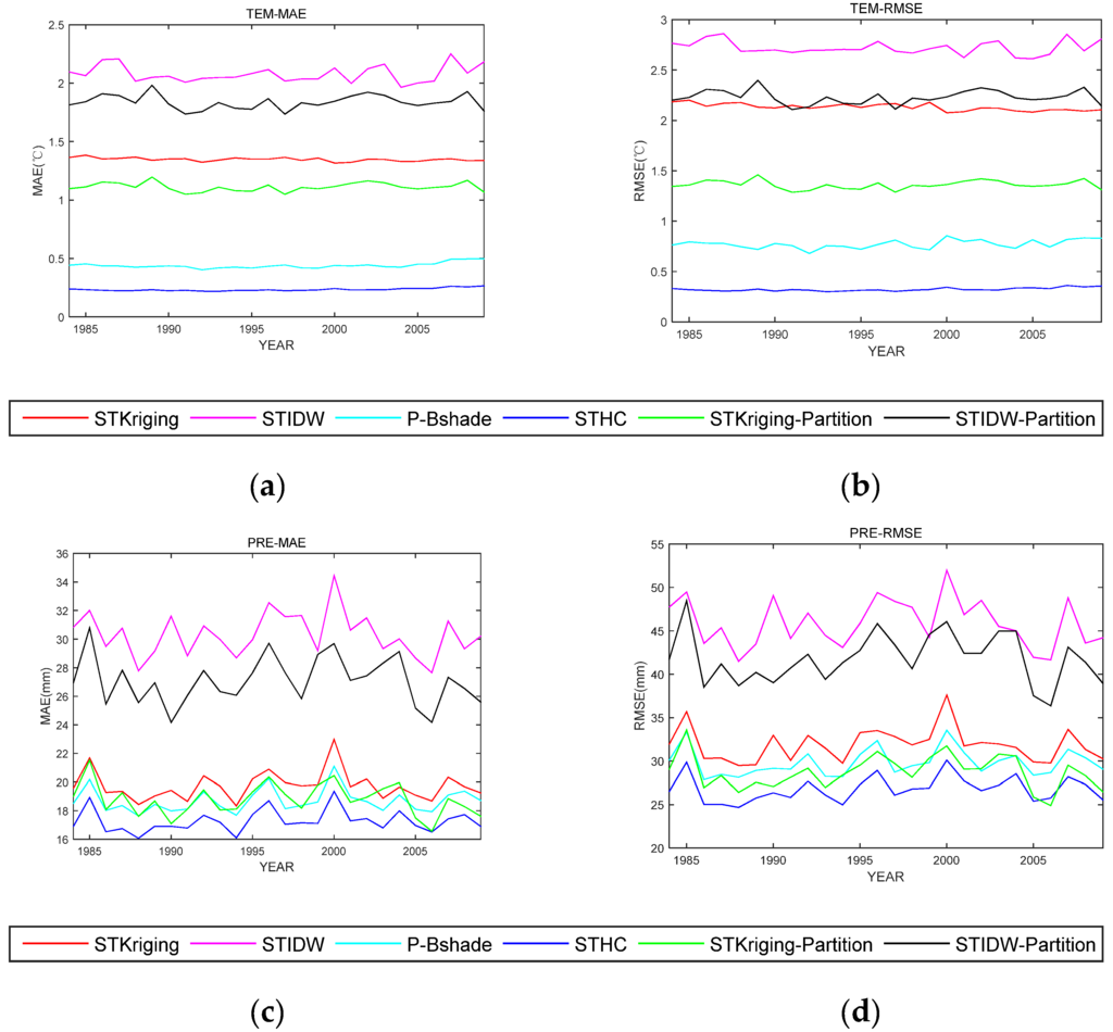
Figure 6. Yearly MAEs and RMSEs from 1984 to 2009 for different methods. (a) TEM-MAE; (b) TEM-RMSE; (c) PRE-MAE; and (d) PRE-RMSE.

In Figure 7, scatterplots between observed values and the estimated values for each method are shown. The horizontal axis denotes the estimated value, and the vertical axis denotes the observed value. The blue dots depict the scatter of estimated values and observed values, and the red line represents the line y = x. If the estimated values are similar to the observed values, the blue dots should be close to the red line (y = x). It can be seen that, compared with other five methods, the estimated value by our method is much closer to its observed value—i.e., closer to the red reference line. For all the six methods, the interpolation results of the temperature data are all better than the results of the precipitation data.

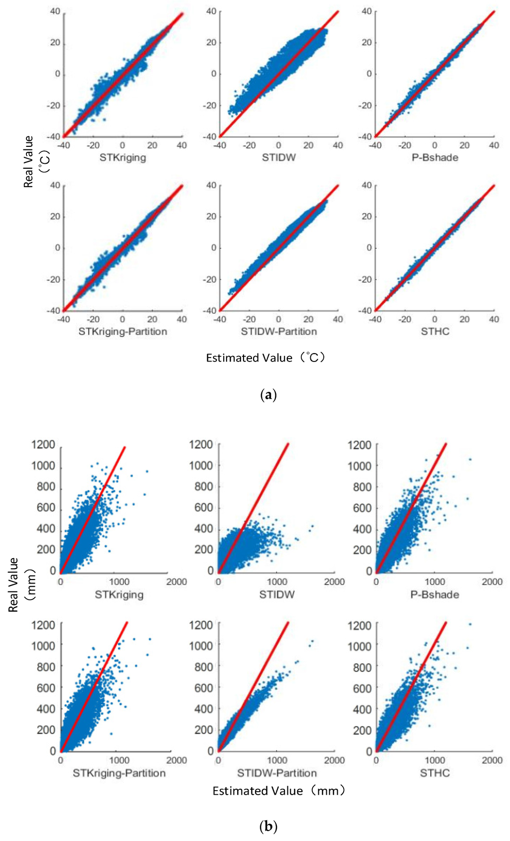
Figure 7. Scatterplot between observed value and the estimated value; (a) temperature and (b) precipitation datasets.

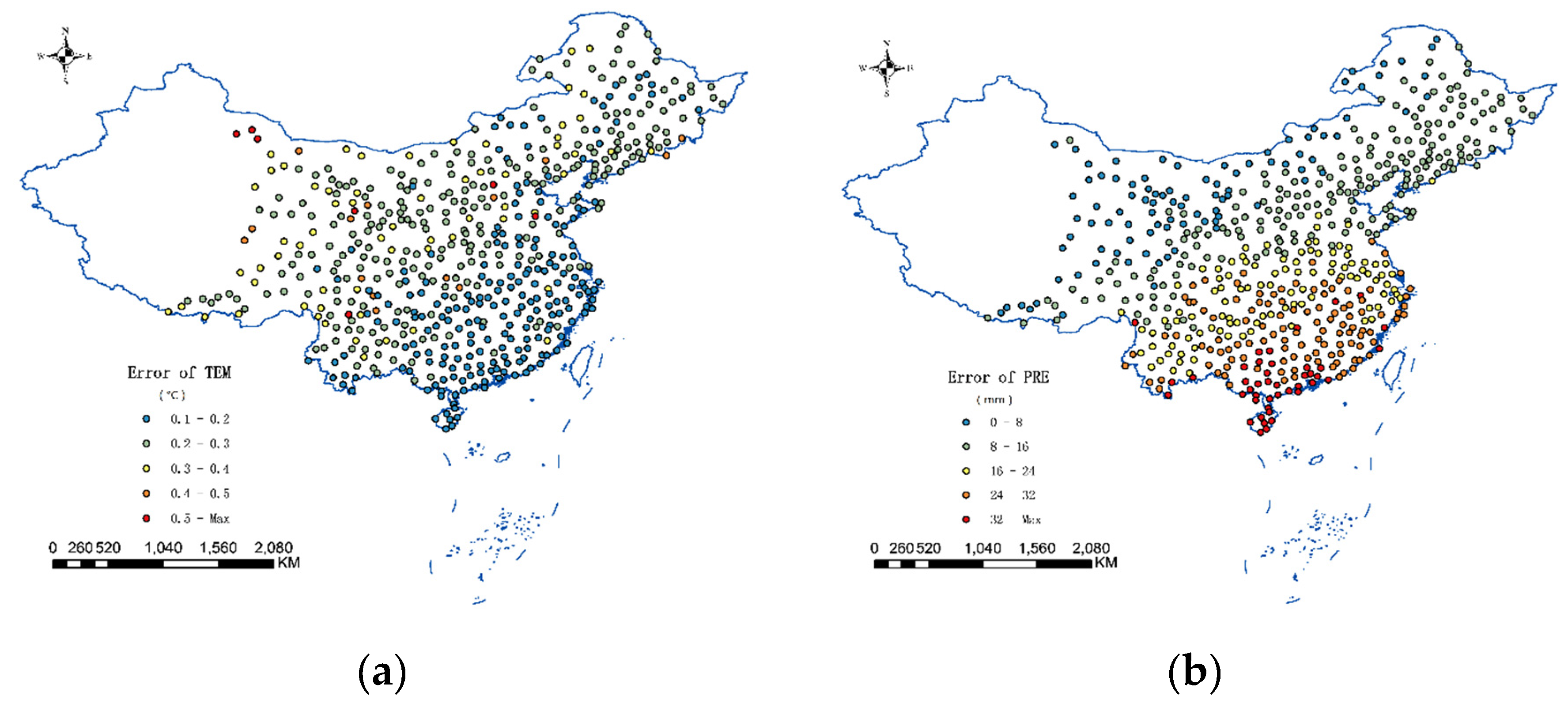
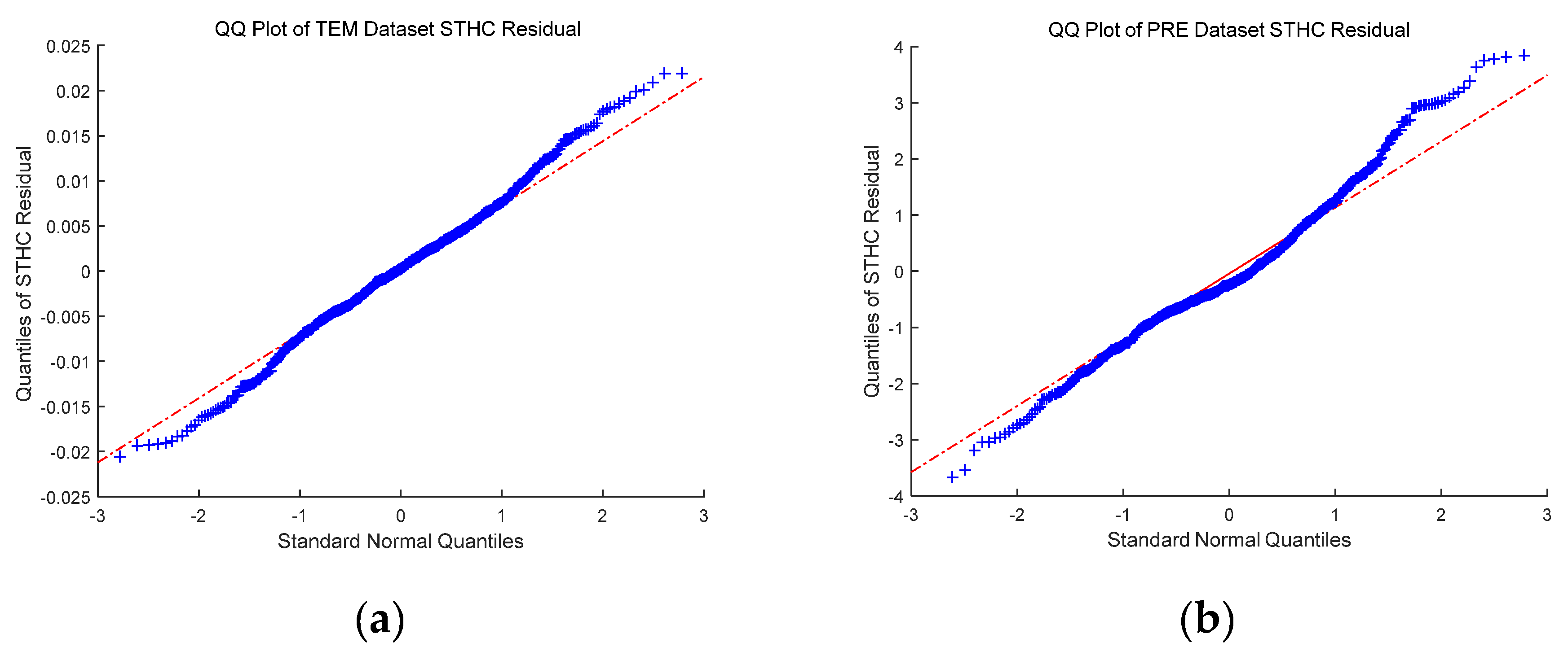
The average interpolation error at each station is plotted in Figure 8. As illustrated in Figure 8a, the error distribution of temperature data is relatively uniform, where Southwest and Northwest China are significantly higher than the eastern region, mainly because the observatory stations in Western China are scarcer. In contrast to the precipitation data, one can see that the errors in Southern China are generally higher than those in Northern China, mainly due to more plentiful rainfall in the south than in the north, which results in increasingly abnormal situations. In Table 1, the residual autocorrelation measured by the Moran’s I index is calculated for each method. It can be found that the proposed method has the least residual autocorrelation. Further, the Quantile-Quantile plot is performed to investigate the normality of the residuals obtained by the proposed method. Based on the results shown in Figure 9, one can find that the plots are close to linear. The kurtosis and skewness are also calculated for the residuals. It can be seen that kurtosis is close to three and skewness is close to zero; thus, it can be concluded that the distribution of the residuals is close to the normal distribution.

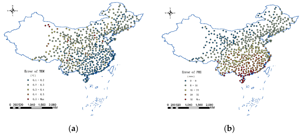
Figure 8. Station srror of the STHC method: (a) temperature data; and (b) precipitation data.

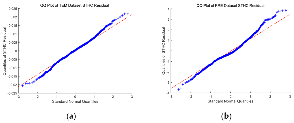
Figure 9. Quantile-Quantile plot of the residuals obtained by the STHC method; (a) temperature data (kurtosis = 3.06, skewness = 0.01); and (b) precipitation data (kurtosis = 3.40, skewness = 0.33).

5. Conclusions

This paper develops a space-time missing data interpolation method based on a heterogeneous spatio-temporal covariance model. Spatial and temporal heterogeneity are first considered in the construction of the covariance model, and the best linear unbiased estimates in spatial and temporal dimensions are obtained. According to the spatio-temporal correlation coefficient, spatial and temporal interpolation results are then integrated to estimate the missing values of the unsampled stations. Experiments and comparisons were performed by using the average annual temperature and precipitation data in China over the past 26 years. The experimental results show that the proposed method achieves higher accuracy than other classic methods.

It should be noted that the space-time interaction may not be fully considered by the proposed method. Although the interpolation results obtained by the proposed method are more accurate than those of existing methods, a space-time coupling model that can fully consider space-time interaction should be developed in the future.

References

- Simpson, G.; Wu, Y. Accuracy and effort of interpolation and sampling: Can GIS help lower field costs? ISPRS Int. J. Geo-Inf. 2014, 3, 1317–1333. [Google Scholar] [CrossRef]
- Simolo, C.; Brunetti, M.; Maugeri, M.; Nanni, T. Improving estimation of missing values in daily precipitation series by a probability density function-preserving approach. Int. J. Climatol. 2010, 30, 1564–1576. [Google Scholar] [CrossRef]
- Curtarelli, M.; Leão, J.; Ogashawara, I.; Lorenzzetti, J.; Stech, J. Assessment of spatial interpolation methods to map the bathymetry of an Amazonian hydroelectric reservoir to aid in decision making for water management. ISPRS Int. J. Geo-Inf. 2015, 4, 220–235. [Google Scholar] [CrossRef]
- Tang, W.Y.; Kassim, A.H.M.; Abubakar, S.H. Comparative studies of various missing data treatment methods—Malaysian experience. Atmos. Res. 1996, 42, 247–262. [Google Scholar] [CrossRef]
- Xu, C.-D.; Wang, J.-F.; Hu, M.G.; Li, Q. Interpolation of missing temperature data at meteorological stations using P-BSHADE. J. Clim. 2013, 26, 7452–7463. [Google Scholar] [CrossRef]
- De Cesare, L.; Myers, D.E.; Posa, D. Estimating and modeling space-time correlation structures. Stat. Probab. Lett. 2001, 51, 9–14. [Google Scholar] [CrossRef]
- Kyriakidis, P.C.; Journel, A.G. Geostatistical space-time models: A review. Math. Geol. 1999, 31, 651–684. [Google Scholar] [CrossRef]
- Kilibarda, M.; Tadic, M.P.; Hengl, T.; Lukovic, J.; Bajat, B. Publicly Available Global Meteorological Data Sets: Sources, Representation, and Usability for Spatio-temporal Analysis. Available online: http://dailymeteo.org/content/publicly-available-global-meteorological-data-sets-sources-representation-and-usability (accessed on 30 November 2015).
- Wang, J.; Xu, C.; Hu, M.; Li, Q.; Yan, Z.; Zhao, P.; Jones, P. A new estimate of the China temperature anomaly series and uncertainty assessment in 1900–2006. J. Geophys. Res.: Atmos. 2014, 119, 1–9. [Google Scholar] [CrossRef]
- De Iaco, S.; Myers, D.E.; Posa, D. Space-time variograms and a functional form for total air pollution measurements. Comput. Stat. Data Anal. 2002, 41, 311–328. [Google Scholar] [CrossRef]
- Li, L.; Revesz, P. Interpolation methods for spatio-temporal geographic data. Comput. Environ. Urban Syst. 2004, 28, 201–227. [Google Scholar] [CrossRef]
- Huang, B.; Wu, B.; Barry, M. Geographically and temporally weighted regression for modeling space-time variation in house prices. Int. J. Geogr. Inf. Sci. 2010, 24, 383–401. [Google Scholar] [CrossRef]
- Cressie, N.A.C. Statistics for Spatial Data; Wiley: Hoboken, NJ, USA, 1993. [Google Scholar]
- Dutilleul, P.R.L. Spatio-Temporal Heterogeneity: Concepts and Analyses; Cambridge University Press: Cambridge, UK, 2011. [Google Scholar]
- Goovaerts, P. Geostatistics for Natural Resources Evaluation; Oxford University Press: Oxford, UK, 1997. [Google Scholar]
- Anselin, L.; Bera, A.K.; Florax, R.; Yoon, M.J. Simple diagnostic tests for spatial dependence. Reg. Sci. Urban Econ. 1996, 26, 77–104. [Google Scholar] [CrossRef]
- Fotheringham, S.; Charlton, M.; Brunsdon, C. Geographically weighted regression: A natural evolution of the expansion method for spatial data analysis. Environ. Plan. A 1998, 30, 1905–1927. [Google Scholar] [CrossRef]
- Erdoğan, S. Modelling the spatial distribution of DEM error with geographically weighted regression: An experimental study. Comput. Geosci. 2010, 36, 34–43. [Google Scholar] [CrossRef]
- Lu, B.; Charlton, M.; Harris, P.; Fotheringham, A.S. Geographically weighted regression with a non-Euclidean distance metric: A case study using hedonic house price data. Int. J. Geogr. Inf. Sci. 2014, 28, 660–681. [Google Scholar] [CrossRef]
- Hubbard, K.G.; Goddard, S.; Sorensen, W.D.; Wells, N.; Osugi, N.N. Performance of quality assurance procedures for an applied climate information system. J. Atmos. Ocean. Technol. 2005, 22, 105–112. [Google Scholar] [CrossRef]
- Hubbard, K.G.; You, J. Sensitivity analysis of quality assurance using the spatial regression approach—A case study of the maximum/minimum air temperature. J. Atmos. Ocean. Technol. 2005, 22, 1520–1530. [Google Scholar] [CrossRef]
- Bartier, P.M.; Keller, C.P. Multivariate interpolation to incorporate thematic surface data using inverse distance weighting (IDW). Comput. Geosci. 1996, 22, 795–799. [Google Scholar] [CrossRef]
- Lu, G.Y.; Wong, D.W. An adaptive inverse-distance weighting spatial interpolation technique. Comput. Geosci. 2008, 34, 1044–1055. [Google Scholar] [CrossRef]
- Reynolds, K.M.; Madden, L.V. Analysis of epidemics using spatio-temporal autocorrelation. Phytopathology 1988, 78, 240–246. [Google Scholar] [CrossRef]
- Furrer, R.; Genton, M.G.; Nychka, D. Covariance tapering for interpolation of large spatial datasets. J. Comput. Graph. Stat. 2006, 15, 502–523. [Google Scholar] [CrossRef]
- Pardo-Iguzquiza, E.; Chica-Olmo, M. Geostatistics with the Matern semivariogram model: A library of computer programs for inference, Kriging and simulation. Comput. Geosci. 2008, 34, 1073–1079. [Google Scholar] [CrossRef]
- Pesquer, L.; Cortés, A.; Pons, X. Parallel ordinary Kriging interpolation incorporating automatic variogram fitting. Comput. Geosci. 2011, 37, 464–473. [Google Scholar] [CrossRef]
- Bhattacharjee, S.; Mitra, P.; Ghosh, S.K. Spatial interpolation to predict missing attributes in GIS using semantic Kriging. IEEE Trans. Geosci. Remote Sens. 2014, 52, 4771–4780. [Google Scholar] [CrossRef]
- Ma, C. Spatio-temporal covariance functions generated by mixtures. Math. Geol. 2002, 34, 965–975. [Google Scholar] [CrossRef]
- Ma, C. Recent developments on the construction of spatio-temporal covariance models. Stochast. Environ. Res. Risk Assess. 2008, 22, 39–47. [Google Scholar] [CrossRef]
- De Iaco, S.; Myers, D.E.; Posa, D. Space-time analysis using a general product-sum model. Stat. Probab. Lett. 2001, 52, 21–28. [Google Scholar] [CrossRef]
- De Iaco, S.; Myers, D.E.; Posa, D. Non-separable space-time covariance models: Some parametric families. Math. Geol. 2002, 34, 23–42. [Google Scholar] [CrossRef]
- De Cesare, L.; Myers, D.E.; Posa, D. Product-sum covariance for space-time modeling: An environmental application. Environmetrics 2001, 12, 11–23. [Google Scholar] [CrossRef]
- Hu, M.-G.; Wang, J.-F.; Zhao, Y.; Jia, L. A B-SHADE based best linear unbiased estimation tool for biased samples. Environ. Model. Softw. 2013, 48, 93–97. [Google Scholar] [CrossRef]
- Wang, J.-F.; Li, X.-H.; Christakos, G.; Liao, Y.-L.; Zhang, T.; Gu, X.; Zheng, X.-Y. Geographical detectors-based health risk assessment and its application in the neural tube defects study of the Heshun region, China. Int. J. Geogr. Inf. Sci. 2010, 24, 107–127. [Google Scholar] [CrossRef]
- Guo, D. Regionalization with dynamically constrained agglomerative clustering and partitioning (REDCAP). Int. J. Geogr. Inf. Sci. 2008, 22, 801–823. [Google Scholar] [CrossRef]
- Kupfer, J.A.; Gao, P.; Guo, D. Regionalization of forest pattern metrics for the continental United States using contiguity constrained clustering and partitioning. Ecol. Inf. 2012, 9, 11–18. [Google Scholar] [CrossRef]
- Pelletier, B.; Dutilleul, P.; Larocque, G.; Fyles, J.W. Coregionalization analysis with a drift for multi-scale assessment of spatial relationships between ecological variables 1. Estimation of drift and random components. Environ. Ecol. Stat. 2009, 16, 439–466. [Google Scholar] [CrossRef]
- Kohavi, R. A study of cross-validation and bootstrap for accuracy estimation and model selection. In Proceedings of the 14th International Joint Conference on Artificial, Montreal, QC, Canada, 20–25 August 1995; pp. 1137–1145.
© 2016 by the authors; licensee MDPI, Basel, Switzerland. This article is an open access article distributed under the terms and conditions of the Creative Commons by Attribution (CC-BY) license (http://creativecommons.org/licenses/by/4.0/).