Dam Deformation Monitoring Data Analysis Using Space-Time Kalman Filter

Abstract

Noise filtering, data predicting, and unmonitored data interpolating are important to dam deformation data analysis. However, traditional methods generally process single point monitoring data separately, without considering the spatial correlation between points. In this paper, the Space-Time Kalman Filter (STKF), a dynamic spatio-temporal filtering model, is used as a spatio-temporal data analysis method for dam deformation. There were three main steps in the method applied in this paper. The first step was to determine the Kriging spatial fields based on the characteristics of dam deformation. Next, the observation noise covariance, system noise covariance, the initial mean vector state, and its covariance were estimated using the Expectation Maximization algorithm (EM algorithm) in the second step. In the third step, we filtered the observation noise, interpolated the whole dam unmonitored data in space and time domains, and predicted the deformation for the whole dam using the Kalman filter recursion algorithm. The simulation data and Wuqiangxi dam deformation monitoring data were used to verify the STKF method. The results show that the STKF not only can filter the deformation data noise in both the temporal and spatial domain effectively, but also can interpolate and predict the deformation for the whole dam.

1. Introduction

Water pressure, temperature, geological condition, construction quality, and other causes bring structural damage to dams, threatening the life of people living in the surrounding area. Dam deformation monitoring and its data processing are effective ways to assess dam safety and avoid possible dam failures [1]. Kalman filter, an effective data processing method for dynamic systems, has been widely used in deformation monitoring data processing [2,3], and improved Kalman filter methods, such as the Kalman filter for colored measurement noise and the robust Kalman filter, have been developed for deformation data analysis [4,5,6]. However, all these applications are based on single point monitoring data series, without considering the spatial correlation between monitoring points. So in some sense, neither the standard nor the improved Kalman filters suit the data analysis of dam deformation, which should be considered as a whole deformation body [7,8]. Furthermore, with the development of modern deformation monitoring technologies, such as Interferometric Synthetic Aperture Radar (InSAR), the observed deformation data can provide more spatio-temporal characteristics of deformation bodies. As such, it is imperative that new data analysis methods are developed to process the deformation data of all monitoring sites as a whole deformation body in both space and time domains.

The Space-Time Kalman Filter (STKF), proposed in the 1990s [9,10,11,12], is a spatio-temporal data processing method combining the Kalman filter and geostatistics models. The commonly used geostatistics model is the Kriging model, so the STKF is also called the Kriged Kalman Filter (KKF) [12]. To overcome the difficulties caused by large datasets and the modeling of spatio-temporal interactions in KKF, a dimension-reduced STKF was developed [13,14]. Distributed Kriged Kalman Filter (DKKF) [15] and Bayesian Kriged Kalman Filter (BKKF) [16,17,18] were proposed later. Current applications of STKF mainly focus on environmental issues. Mardia et al. (1998) employed KKF in dealing with the distribution of Sulphur dioxide in Leeds [12]. Wikle et al. (1999) validated the STKF model with a dataset of near-surface tropical winds [13]. Sahu et al. (2005) applied STKF to model atmospheric particulate distribution in New York in the USA and made a short-term prediction [16]. Lasinio et al. (2005) established a spatio-temporal rainfall model which includes seasonality and covariates based BKKF [17]. Al-Awadhi et al. (2012) used regression and BKKF to predict average hourly concentration of non-methane hydrocarbons in unmonitored areas of Kuwait [18]. Qing et al. (2012) adopted BKKF for short-term wind speed predictions [19]. However, STKF is quite rarely used in deformation data analysis. As such, this paper brings the STKF to the deformation analysis of dam.

In this paper, we first introduce the mathematical model of STKF. Then, the methods and algorithms to determine the Kriging spatial fields and parameters of STKF for the dam deformation data analysis are presented in detail. Then, we apply a STKF model to filter the noise, interpolate deformation data for the whole dam both in space and time domains, and make a short-term prediction. Finally, experiments with simulation data and real dam horizontal displacement monitoring data are conducted to verify the STKF model.

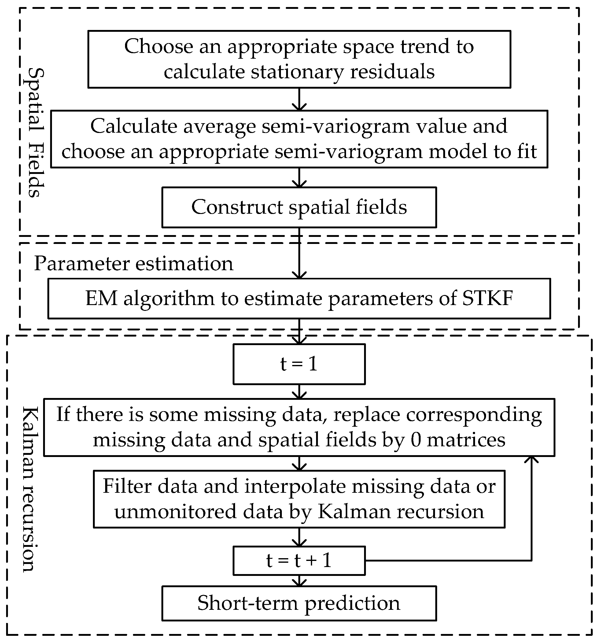
2. Space-Time Kalman Filter Model

In this part, the mathematical model of STKF is introduced in Section 2.1. Section 2.2 shows how to construct the spatial fields of STKF using the Kriging model. In Section 2.3, we discuss briefly the Expectation Maximization algorithm (EM algorithm) for parameter estimation. In the last section, we review the Kalman Filter recursion steps and methods of interpolating and predicting deformation in space and time.

2.1. Mathematical Model

Given location points $\left\{\mathrm{s}={\mathrm{s}}_1,{\mathrm{s}}_2,\dots ,{\mathrm{s}}_n\right\}$ and time points $\left\{t=1,2,\dots ,m\right\}$, observation value $L_t\left(\mathrm{s}\right)$ can be decomposed into mean and observed error components [14]:

$$L_t\left(\mathrm{s}\right)=Y_t\left(\mathrm{s}\right)+{\epsilon }_t\left(\mathrm{s}\right),$$

(1)

where ${\epsilon }_t\left(\mathrm{s}\right)$ is the observed error components and $Y_t\left(\mathrm{s}\right)$ is the mean component. $Y_t\left(\mathrm{s}\right)$ can be expressed as a time-varying linear combination $\mathit{\alpha }\left(t\right)\left(p\times 1\right)$ of spatial fields $h\left(s\right)\left(p\times 1\right)$ [12], which can be written as

$$Y_t\left(s\right)=h_1\left(s\right){\alpha }_1\left(t\right)+h_2\left(s\right){\alpha }_2\left(t\right)+\cdots +h_p\left(s\right){\alpha }_p\left(t\right)=h{\left(s\right)}^T\mathit{\alpha }\left(t\right),$$

(2)

where ${(\ast )}^T$ is the transpose operator and the vector $\mathit{\alpha }\left(t\right)$ is the state for $Y_t\left(s\right)$, representing the dynamic time components. Generally speaking, $p\ll n$, so the number of $p$ is the key to reduce the dimension of the space domain.

Writing $H=\left[h{\left({\mathrm{s}}_1\right)}^T;h{\left({\mathrm{s}}_2\right)}^T;\dots ;h{\left({\mathrm{s}}_n\right)}^T\right]$, ${\mathit{L}}_t={\left[L_t\left({\mathrm{s}}_1\right),L_t\left({\mathrm{s}}_2\right),\dots ,L_t\left({\mathrm{s}}_n\right)\right]}^T$, and ${\mathit{\epsilon }}_t={\left[{\epsilon }_t\left({\mathrm{s}}_1\right),{\epsilon }_t\left({\mathrm{s}}_2\right),\dots ,{\epsilon }_t\left({\mathrm{s}}_n\right)\right]}^T$, the substitution of (2) into (1) gives the observation Equation (3) of STKF.

$${\mathit{L}}_t=H\mathit{\alpha }\left(t\right)+{\mathit{\epsilon }}_t$$

(3)

The state equation can be shown by

$$\mathit{\alpha }\left(t\right)=\mathsf{\Phi }\mathit{\alpha }\left(t-1\right)+\mathit{\eta }\left(t\right),$$

(4)

where $\mathsf{\Phi }$ is the state transition matrix, $\mathit{\eta }\left(t\right)$ is the system error at time $t$. Suppose ${\mathit{\epsilon }}_t~\mathrm{N}\left(0,{\mathsf{\Sigma }}_{\epsilon }\right)$, $\mathit{\eta }\left(t\right)~\mathrm{N}\left(0,{\mathsf{\Sigma }}_{\eta }\right)$, where $\mathrm{N}\left(\ast ,\ast \right)$ is the normal distribution operator, ${\mathsf{\Sigma }}_{\epsilon }$ is the observation noise covariance and ${\mathsf{\Sigma }}_{\eta }$ is the system noise covariance.

Equations (3) and (4) form the STKF model. According to the model, matrices $H,\mathsf{\Phi },{\mathsf{\Sigma }}_{\epsilon },{\mathsf{\Sigma }}_{\eta }$ and the initial state $\mathit{\alpha }\left(0\right)~N\left({\widehat{\mathit{a}}}_{0|0},P_{0|0}\right)$ are essential to implement the STKF recursion. The spatial fields $H$ are built by spatial Kriging fields which is the key to take spatial correlation into consideration. Parameter $\theta =\left\{{\widehat{\mathit{a}}}_{0|0},P_{0|0},\mathsf{\Phi },{\mathsf{\Sigma }}_{\epsilon },{\mathsf{\Sigma }}_{\eta }\right\}$ can be estimated by the EM algorithm. In the following sections, we will present the method to obtain these matrices in detail.

2.2. Spatial Fields $H$

Spatial fields $H$ are built by spatial Kriging model. At time point $t$ the universal Kriging model is as follows:

$$Y_t\left(s\right)={\mathit{f}}^T\left(s\right){\beta }_t+{\varsigma }_t\left(s\right),$$

(5)

where $\mathit{f}\left(s\right)={\left[f_1\left(s\right),f_2\left(s\right),\mathrm{..}{f}_q\left(s\right)\right]}^T$ is the given space trend fields, whose elements are a function of the coordinate of $s$. Commonly used space trend fields are constant, linear and quadratic trends. The subscript $q$ is determined by the chosen trend. ${\beta }_t$ is the coefficient of $\mathit{f}\left(s\right)$, and ${\varsigma }_t\left(s\right)$ is the local space variation after removing space trend. Assume ${\varsigma }_t\left(s\right)$ is stationary, and it can be described by the spatial covariance (or semi-variogram) model [14,16]. An empirical semi-variogram model can be obtained from the observations to describe ${\varsigma }_t\left(s\right)$. First, calculate the detrended data ${\mathit{D}}_t$ at time point $t$ by ordinary least squares,

$${\mathit{D}}_t={\mathit{Y}}_t-F{(F^{T}F)}^{-1}{F}^T{\mathit{Y}}_t,$$

(6)

where ${(\ast )}^{-1}$ is the inverse operator, ${\mathit{D}}_t={\left[D_t\left({\mathrm{s}}_1\right),D_t\left({\mathrm{s}}_2\right),\dots ,D_t\left({\mathrm{s}}_n\right)\right]}^T$, ${\mathit{Y}}_t={\left[Y_t\left({\mathrm{s}}_1\right),Y_t\left({\mathrm{s}}_2\right),\dots ,Y_t\left({\mathrm{s}}_n\right)\right]}^T$, and $F=\left[\mathit{f}{\left(s_1\right)}^T;f{\left(s_2\right)}^T;\dots ;\mathit{f}{\left(s_n\right)}^T\right]$ is the chosen trend matrix. Here, assuming $F$ does not change with time, the empirical semi-variogram can be estimated by average semi-variogram,

$$\widehat{\mathsf{\gamma }}\left(d\right)=\frac{1}{2m}{\sum }_{t=1}^m{\left[D_t\left(s\right)-D_t\left(s+d\right)\right]}^2,$$

(7)

where ${\sum }_{\ast }^{\ast }(\ast )$ is the sum operator. Choose a semi-variogram model to fit $\widehat{\mathsf{\gamma }}\left(d\right)$, and spatial covariance can be obtained by ${\sigma }_{\varsigma }\left(s_i,s_j\right)=C-\widehat{\mathsf{\gamma }}(\Vert s_i-s_j\Vert )$, where $C$ is the sill value of semi-variogram model and $\Vert \ast \Vert$ is the distance operator.

After choosing the space trend fields and fixing the semi-variogram function, the Kriging predictor can be written as follows [20,21]:

$${\widehat{Y}}_t\left(s\right)=\mathit{f}{\left(s\right)}^{T}A{\mathit{Y}}_t+{\mathit{\sigma }}_{\varsigma }{\left(s\right)}^{T}B{\mathit{Y}}_t,$$

(8)

where ${\mathit{\sigma }}_{\varsigma }\left(s\right)={\left[{\sigma }_{\varsigma }\left(s,s_1\right),{\sigma }_{\varsigma }\left(s,s_2\right),\dots ,{\sigma }_{\varsigma }\left(s,s_n\right)\right]}^T$. Matrices $A$ and $B$ have the fixed form as

$$A={\left(F^T{\mathsf{\Sigma }}_{\varsigma }^{-1}F\right)}^{-1}{F}^T{\mathsf{\Sigma }}_{\varsigma }^{-1},$$

(9)

$$B={\mathsf{\Sigma }}_{\varsigma }^{-1}-{\mathsf{\Sigma }}_{\varsigma }^{-1}FA,$$

(10)

where ${\mathsf{\Sigma }}_{\varsigma }$ is a spatial covariance matrix with ${\left({\mathsf{\Sigma }}_{\varsigma }\right)}_{ij}={\sigma }_{\varsigma }\left(s_i,s_j\right)$, and $B$ is known as the bending energy matrix [12,22], which is used to describe the scale of local space variation after removing space trend. For dimension reduction, consider the spectral decomposition of matrix $B$,

$$B=UD{U}^T,B{u}_i=d_i{u}_i,$$

(11)

where columns of $U=\left[u_1,u_2,\dots ,u_n\right]$ are eigenvectors of $B$, and diagonal elements of $D=\mathrm{diag}\left(d_1,d_2,\mathrm{..},d_n\right)$ are corresponding eigenvalues, and $\mathrm{diag}(\ast )$ is the diagonal matrix operator. It is easy to verify that $BF=0$, which means columns of $F$ can be thought as the eigenvectors of $B$ with corresponding zero eigenvalues $d_1,d_2,\mathrm{..},d_q$. Obviously, smaller eigenvalues show larger scale space variations, while larger eigenvalues describe the local spatial variations [16].

The eigenvectors $u_i$ form a set of orthogonal basis, so the mean vector ${\mathit{Y}}_t$ can be represented as a linear combination of the eigenvectors $u_i$. Indeed, suppose that ${\mathit{Y}}_t={\sum }_{i=1}^n{c}_{i,t}{u}_i,{\widehat{\beta }}_t=A{\mathit{Y}}_t$ and Equation (8) can be rewritten as

$${\widehat{Y}}_t\left(s\right)=\mathit{f}{\left(s\right)}^T{\widehat{\beta }}_t+{\displaystyle \sum }_{i=q+1}^n{c}_{i,t}{d}_i{\mathit{\sigma }}_{\varsigma }{\left(s\right)}^T{u}_i=h{\left(s\right)}^T\left[\begin{array}{c}{\widehat{\beta }}_t\\ {\mathit{c}}_{\mathit{t}}\end{array}\right]$$

(12)

where ${\mathit{c}}_{\mathit{t}}={\left[c_{q+1,t},\mathrm{..},c_{n,t}\right]}^T$. If $n$ is very large, we only take the first $p$ space variations to reduce dimension, which results spatial fields in the form of dimensionality reduction (13). Parameter $p$ can be obtained while the ratio $e={\sum }_{i=1}^p{d}_i∕{\sum }_{i=1}^n{d}_i$ exceeds a certain percentage (usually 90% or 95%) [18], which explains the proportion that the selected spatial variations take in the total spatial variation.

$$\begin{array}{c}{h}_i\left(s\right)=f_i\left(s\right),\mathrm{for} i=1,2,\dots ,q\\ h_j\left(s\right)=d_j{\mathit{\sigma }}_{\varsigma }{\left(s\right)}^T{u}_j,\mathrm{for} j=q+1,\dots ,p\end{array}$$

(13)

It is worth noting that $h_i\left(s\right)=f_i\left(s\right)$ is the trend field used to describe the global trend. $h_j\left(s\right)=d_j{\mathit{\sigma }}_{\varsigma }{\left(s\right)}^T{u}_j$ is the principal field used to grasp local spatial variation. If ignoring the principal field, STKF will reduce to a spatio-temporal trend surface model [16], and if continuously taking $h_i\left(s\right)=f_i\left(s\right)=1$, STKF will reduce to a standard Kalman model. Also, if only taking observation equation of STKF into consideration, STKF will reduce to a universal Kriging model.

2.3. Parameters Estimation

The maximum likelihood estimation (MLE) is an effective way to estimate parameter $\theta =\left\{{\widehat{\mathit{a}}}_{0|0},P_{0|0},\mathsf{\Phi },{\mathsf{\Sigma }}_{\epsilon },{\mathsf{\Sigma }}_{\eta }\right\}$. However, from the logarithm of joint likelihood function (14), we cannot maximize directly the logarithm of joint likelihood function $\log \left(l\right)$ because of the unknown distribution of state vector $\mathit{\alpha }(t)$.

$$\begin{array}{l}\log (l)=-\frac{1}{2}\log \left|P_{0|0}\right|-\frac{1}{2}{(\mathit{\alpha }\left(0\right)-{\widehat{\mathit{\alpha }}}_{0|0})}^T{P}_{0|0}^{-1}(\mathit{\alpha }\left(0\right)-{\widehat{\mathit{\alpha }}}_{0|0})\\ -\frac{m}{2}\log \left|{\mathsf{\Sigma }}_{\eta }\right|-\frac{1}{2}{\sum }_{t=1}^m{(\mathit{\alpha }\left(t\right)-\mathsf{\Phi }\mathit{\alpha }(t-1))}^T{\mathsf{\Sigma }}_{\eta }^{-1}(\mathit{\alpha }\left(t\right)-\mathsf{\Phi }\mathit{\alpha }(t-1))\\ -\frac{m}{2}\log \left|{\mathsf{\Sigma }}_{\epsilon }\right|-\frac{1}{2}{\sum }_{t=1}^m({{\mathit{L}}_t-H\mathit{\alpha }\left(t\right))}^T{\mathsf{\Sigma }}_{\epsilon }^{-1}({\mathit{L}}_t-H\mathit{\alpha }(t))\end{array},$$

(14)

where $|\ast |$ is the determinant operator and $\log (\ast )$ is the logarithm operator.

The EM algorithm provides an iterative method to maximize $\log \left(l\right)$, which consists of Expectation Step (E step) and Maximization Step (M step) [23]. Suppose it is in the $\left(r+1\right)th$ iteration, then the main steps of EM algorithm are as follows:

• Use Kalman smoother to estimate the unknown state parameter $\mathit{\alpha }\left(t\right)$ with respect to the $\left(r\right)th$ iterated value ${\theta }_r$.
• E step: calculate the conditional expectation $\mathrm{G}\left({\theta }_r\right)=E(\log \left(l\right)|{\mathit{L}}_1,{\mathit{L}}_2,\mathrm{..},{\mathit{L}}_m)$ of $\log \left(l\right)$ under the estimated $\mathit{\alpha }\left(t\right)$ distribution in step 1, where $E(\ast )$ is the expectation operator.
• M step: maximize $\mathrm{G}\left({\theta }_r\right)$, which yields the newly iterated value ${\theta }_{r+1}$.
• Replace ${\theta }_r$ with ${\theta }_{r+1}$, and repeat steps 1, 2, and 3 until the logarithm of joint likelihood function $\log \left(l\right)$ or the innovations form [23] stop increasing.

2.4. Denoising, Space-Time Interpolation, and Prediction

As matrix $H$ and parameter $\theta$ are estimated, Kalman filter recursion can be conducted. It should be noted that the STKF model needs no preprocessing, such as the interpolation of missing data, which can be dynamically calculated while filtering the noise. Suppose at time point $t$, the observation equation is as follows:

$$\left(\begin{array}{c}{L}_t^1\\ L_t^2\end{array}\right)=\left(\begin{array}{c}{H}^1\\ H^2\end{array}\right)\mathit{\alpha }\left(t\right)+\left(\begin{array}{c}{\epsilon }_t^1\\ {\epsilon }_t^2\end{array}\right),$$

(15)

where ${\mathit{L}}_t^1$, $H^1,$ and ${\mathit{\epsilon }}_t^1$ are the observed data, spatial fields, and errors of observed data, respectively, and ${\mathit{L}}_t^2$, $H^2$, and ${\mathit{\epsilon }}_t^2$ are the missing data, spatial fields, and errors of missing data, respectively. In order to implement Kalman recursion, setting ${\mathit{L}}_t^2$ and $H_t^2$ to zero matrix [23], the estimation of $\mathit{\alpha }\left(t\right)$ can be obtained by

$$\begin{array}{ll}{\widehat{\mathit{\alpha }}}_{t|t}& =E\left(\mathit{\alpha }\left(t\right)|{\mathit{L}}_1,{\mathit{L}}_2,\dots ,{\mathit{L}}_t\right)\\ & ={\widehat{\mathit{\alpha }}}_{t|t-1}+G_t\left({\mathit{L}}_t-H{\widehat{\mathit{\alpha }}}_{t|t-1}\right)\end{array},$$

(16)

and its mean-squared-prediction-error matrix

$$\begin{array}{ll}{P}_{t|t}& =E[\left({\widehat{\mathit{\alpha }}}_{t|t}-\mathit{\alpha }\left(t\right)\right){\left({\widehat{\mathit{\alpha }}}_{t|t}-\alpha \left(t\right)\right)}^T]\\ & =P_{t|t-1}-G_{t}H{P}_{t|t-1}\end{array},$$

(17)

where the Kalman gain matrix $G_t$ is given by

$$G_t=P_{t|t-1}{H}^T{\left(H{P}_{t|t-1}{H}^T+{\mathsf{\Sigma }}_{\epsilon }\right)}^{-1}.$$

(18)

The one-step-ahead-forecast quantities are given by

$${\widehat{\mathit{\alpha }}}_{t|t-1}=\mathsf{\Phi }{\widehat{\mathit{\alpha }}}_{t-1|t-1},$$

(19)

$$P_{t|t-1}=\mathsf{\Phi }{P}_{t-1|t-1}{\mathsf{\Phi }}^T+{\mathsf{\Sigma }}_{\eta }.$$

(20)

Short-term prediction involves optimal prediction of $Y_t\left(\mathrm{s}\right)$ $\mathrm{from}{\mathit{L}}_1,{\mathit{L}}_2,\dots ,{\mathit{L}}_m$, where $t\mathsf{ϵ}\left\{\mathrm{m}+1,\mathrm{m}+2,\dots \right\}$. Based on the one-step-ahead-forecast Equations (19) and (20), the optimal prediction estimator ${\widehat{\mathit{\alpha }}}_{t|m}$ of $\mathit{\alpha }\left(t\right)$ is

$${\widehat{\mathit{\alpha }}}_{t|m}=E\left(\mathit{\alpha }\left(t\right)|{\mathit{L}}_1,{\mathit{L}}_2,\dots ,{\mathit{L}}_m\right)=({{\displaystyle \prod }}_{i=m+1}^t\mathsf{\Phi }){\widehat{\mathit{\alpha }}}_{m|m},$$

(21)

with its mean-squared-prediction-error matrix

$$\begin{array}{c}{P}_{t|m}=\left({\displaystyle \prod _{i=m+1}^t}\mathsf{\Phi }\right)P_{m|m}{\left({\displaystyle \prod _{i=m+1}^t}\mathsf{\Phi }\right)}^T+{\mathsf{\Sigma }}_{\eta }\\ +{\displaystyle \sum _{i=m+1}^{t-1}}\left\{\left({\displaystyle \prod _{j=m+1}^t}\mathsf{\Phi }\right){\mathsf{\Sigma }}_{\eta }{\left({\displaystyle \prod _{j=m+1}^t}\mathsf{\Phi }\right)}^T\right\}\end{array}$$

(22)

where Π is the multiplication operator. The optimal prediction of $Y_t\left(\mathrm{s}\right)$ can be calculated by ${\widehat{Y}}_t\left(s\right)=h{\left(s\right)}^T{\widehat{\mathit{\alpha }}}_{t|m}$.

After obtaining ${\widehat{\mathit{\alpha }}}_{t|t}$, the optimal estimator of $Y_t\left(s\right)$ at any location point $s$ and time point $t$ of interest can be calculated by

$${\widehat{Y}}_t\left(s\right)=h{\left(s\right)}^T{\widehat{\mathit{\alpha }}}_{t|t},$$

(23)

where $h\left(s\right)$ can be calculated by Equation (13).

Lastly, a flow diagram of the overall procedure of STKF is displayed in Figure 1.

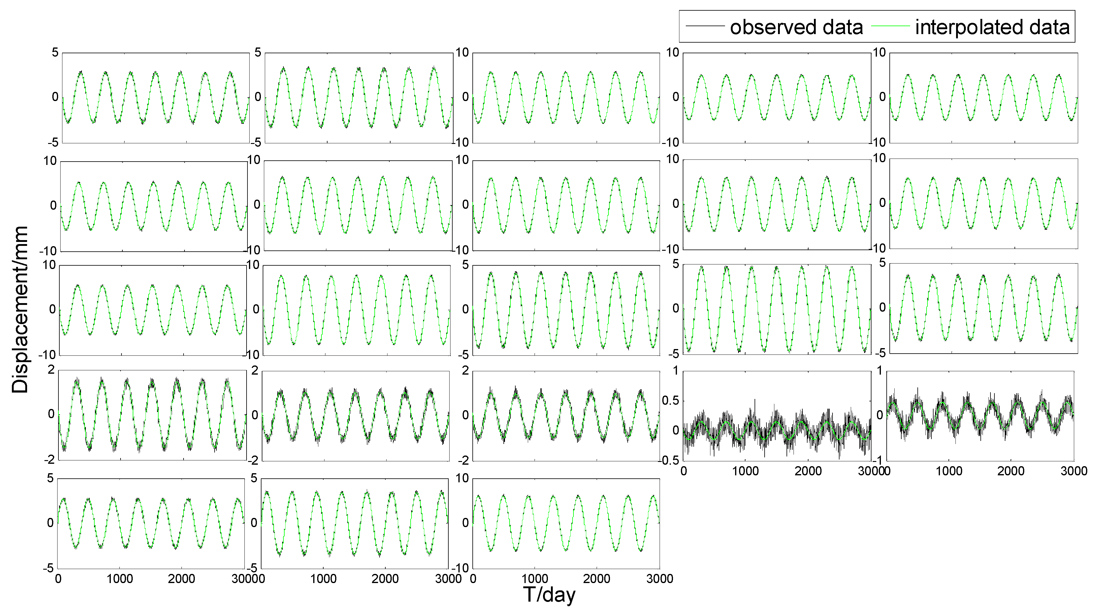
3. Simulation Experiment

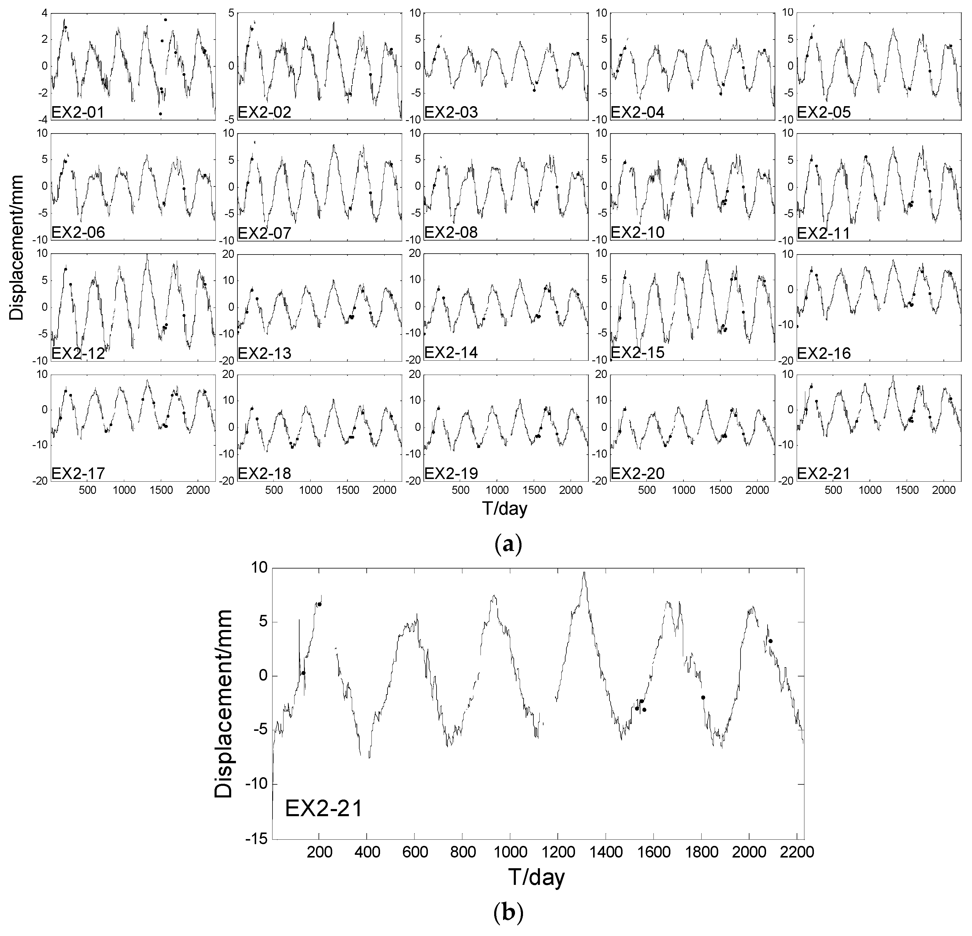
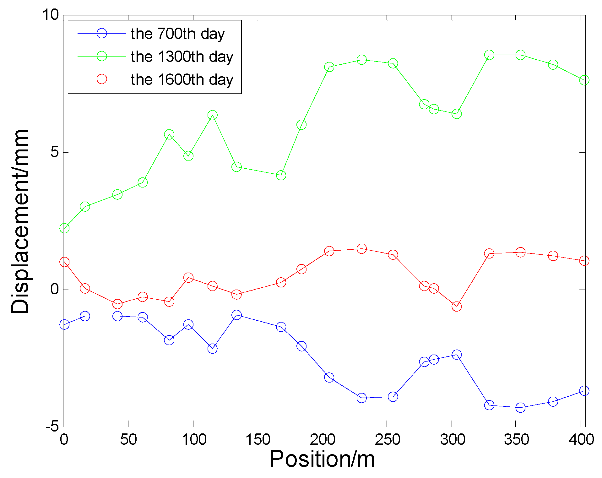
To simulate the horizontal displacement observation data of a dam, we assumed that the horizontal displacement has a quadratic curve trend in space and it changes in a sinusoidal trend in time. The horizontal displacement of a dam in space and time can be described by

$$\mathrm{g}\left(s,t\right)=\left(0.0013s^2-0.04s-2.7\right)\sin \left(0.005\pi t^2-0.00125\pi \right)+\epsilon .$$

(24)

In Equation (24), $\mathrm{g}$ is the displacement, $\mathrm{s}$ is the position of the monitoring points on the dam, $\mathrm{t}$ is the time, and $\epsilon$ is the observation noise with a standard deviation of 0.1 mm. Suppose $s=0\left(m\right)+20k\left(m\right) ,k=0,1,2,\dots ,22$, for 23 points in total, and $t=1\left(day\right)+1j\left(day\right),j=0,1,2,\dots ,2900$, then the horizontal displacement data series (1 day sampling rate) of 23 monitoring points have been simulated.

As mentioned in Section 2.2, in order to acquire the spatial fields $H$, we had to first get the trend matrix $F$. Since the simulation experiment constructs a known space-time curve, the trend field is known as $F=\left[s^2,s,1\right]$. To get the principal fields, it was necessary to choose a suitable spatial semi-variogram model. Commonly used models are the exponential model, Gaussian model, spherical model, and Matèrn family model [20,21]. We chose the spherical model in this experiment as it can maximally show the spatial variation and is the most widely used spatial semi-variogram model [24]. The rest parameter $\theta =\left\{{\widehat{\mathit{a}}}_{0|0},P_{0|0},\mathsf{\Phi },{\mathsf{\Sigma }}_{\epsilon },{\mathsf{\Sigma }}_{\eta }\right\}$ was estimated by the EM algorithm, which is described in Section 2.3.

In the simulation experiment, we used all data to filter the noise firstly. Secondly, in order to verify the effectiveness of the spatio-temporal interpolation using STKF, we randomly sampled one point as the unobserved data, the rest points as the observed data to establish a model and use the established model to interpolate the unobserved displacement. We repeated the sampling process until all monitoring points were interpolated. The interpolation results are shown in Figure 2. Lastly, we predicted three days of horizontal displacement for all points using STKF. The statistic results of filtering, interpolation, and prediction are shown in

Table 1. $RM{S}^1$ of Interpolation, Filter, and Prediction of each point (unit: mm). Interp, Interpolation; Pred, Prediction.

Site	Interp	Filter	Pred	Site	Interp	Filter	Pred	Site	Interp	Filter	Pred
1	0.019	0.022	0.030	9	0.039	0.043	0.059	17	0.014	0.019	0.038
2	0.024	0.025	0.056	10	0.037	0.037	0.073	18	0.009	0.017	0.029
3	0.026	0.029	0.051	11	0.036	0.036	0.077	19	0.004	0.012	0.003
4	0.030	0.032	0.055	12	0.034	0.034	0.068	20	0.008	0.013	0.008
5	0.033	0.035	0.061	13	0.031	0.032	0.064	21	0.015	0.017	0.033
6	0.035	0.035	0.081	14	0.028	0.029	0.055	22	0.023	0.025	0.040
7	0.037	0.037	0.091	15	0.024	0.027	0.042	23	0.032	0.034	0.057
8	0.037	0.037	0.072	16	0.019	0.022	0.038

followed by the statistic model of $RM{S}^1$:

$$RM{S}^1=\sqrt{{\displaystyle \sum }_{i=1}^N{({\widehat{Y}}_i-R_i)}^2/N}$$

(25)

where ${\widehat{Y}}_i$ is the estimated value, $R_i$ is the true value, and $N$ is the number of ${\widehat{Y}}_i$.

As Figure 2 shows, the interpolated values coincided with the observed values. As such, we can say that the STKF can well interpolate the point data without monitoring. As listed in Table 1, the interpolation and filter $RM{S}^1$ was about 0.03 mm, which had been reduced by about 70% compared with the noise whose standard deviation was 0.1 mm. The interpolation result and filter result were very close, which may be due to the fact that we used a very exact trend matrix. For the prediction result, the prediction accuracy was lower than that of filter and interpolation. Its RMS was around 0.05 mm with the maximum value of 0.091 mm, which was close to the standard deviation of 0.1 mm.

4. Application

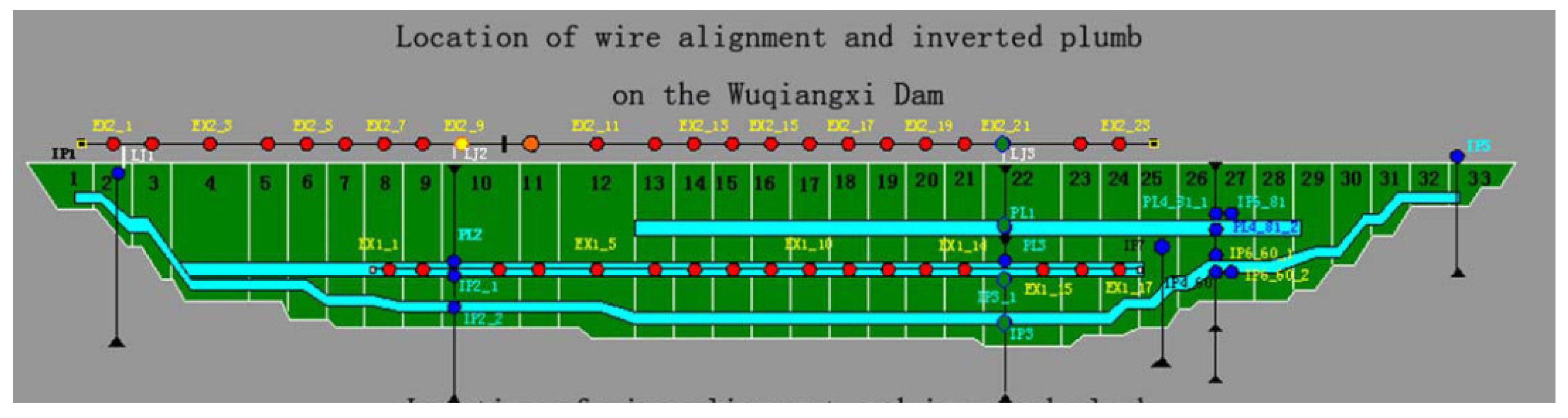
4.1. Description of Wuqiangxi Dam Tension Wire Alignment Data

The real horizontal displacement data came from Wuqiangxi Dam tension wire alignment. Wuqiangxi Dam, located in the main stream of Yuan River in the Yuanling County of Hunan Province, was built in 1994. The dam is a concrete gravity dam with a horizontal length of 724.4 m, a crest height of 85.8 m, and a maximum water reservoir volume of $4.29\times {10}^9{\mathrm{m}}^3$. The left side of the dam is a generator set with a power of $1.2\times {10}^6\mathrm{KW}$ and the right side of the dam is a navigation lock. The foundation of this dam can be divided into four types: sandstone, quartzite, slate, and phyllitic slate. This dam is equipped with the automatic monitoring system of wire alignment, inverted plumbline, hydrostatic levelling, seepage monitoring, uplift pressure monitoring, and water level measuring system [25]. The Wuqiangxi Dam contains two tension wire alignments, EX1 and EX2. We selected the EX2 tension wire alignment data in the experiment, which are composed of 23 measuring points and their unidimensional position information, with their original points lying in the far left of the EX2 tension wire alignment, as presented in

Table 2. Position information of EX2 tension wire alignment measuring points (unit: m).

Site	Position	Site	Position	Site	Position	Site	Position
EX2_1	0.5	EX2_2	17.1	EX2_3	41.6	EX2_4	61.1
EX2_5	81.6	EX2_6	97.1	EX2_7	115.6	EX2_8	134.1
EX2_10	168.6	EX2_11	184.1	EX2_12	205.6	EX2_13	230.2
EX2_14	254.7	EX2_15	279.2	EX2_16	286.2	EX2_17	303.7
EX2_18	329.2	EX2_19	353.7	EX2_20	378.2	EX2_21	402.7

. The displacement data contains 2233 daily observations from 1 July 2004 to 11 August 2010. Figure 3 shows the distribution of the tension wire alignment sites. In our experiment, displacement data of EX2_09, EX2_22, and EX2_23 were excluded due to their poor quality. Figure 4a shows the displacement sequences of all selected points. From Figure 4a, we can conclude that the displacement data has significant seasonal trends in the time domain. In order to extract more information from the observation data, Figure 4b shows the amplification of the displacement data of EX2_21 point. There was a gross error that occurred in the time surrounding the 100th day that resulted in some missing data of varying lengths during the whole displacement sequence.

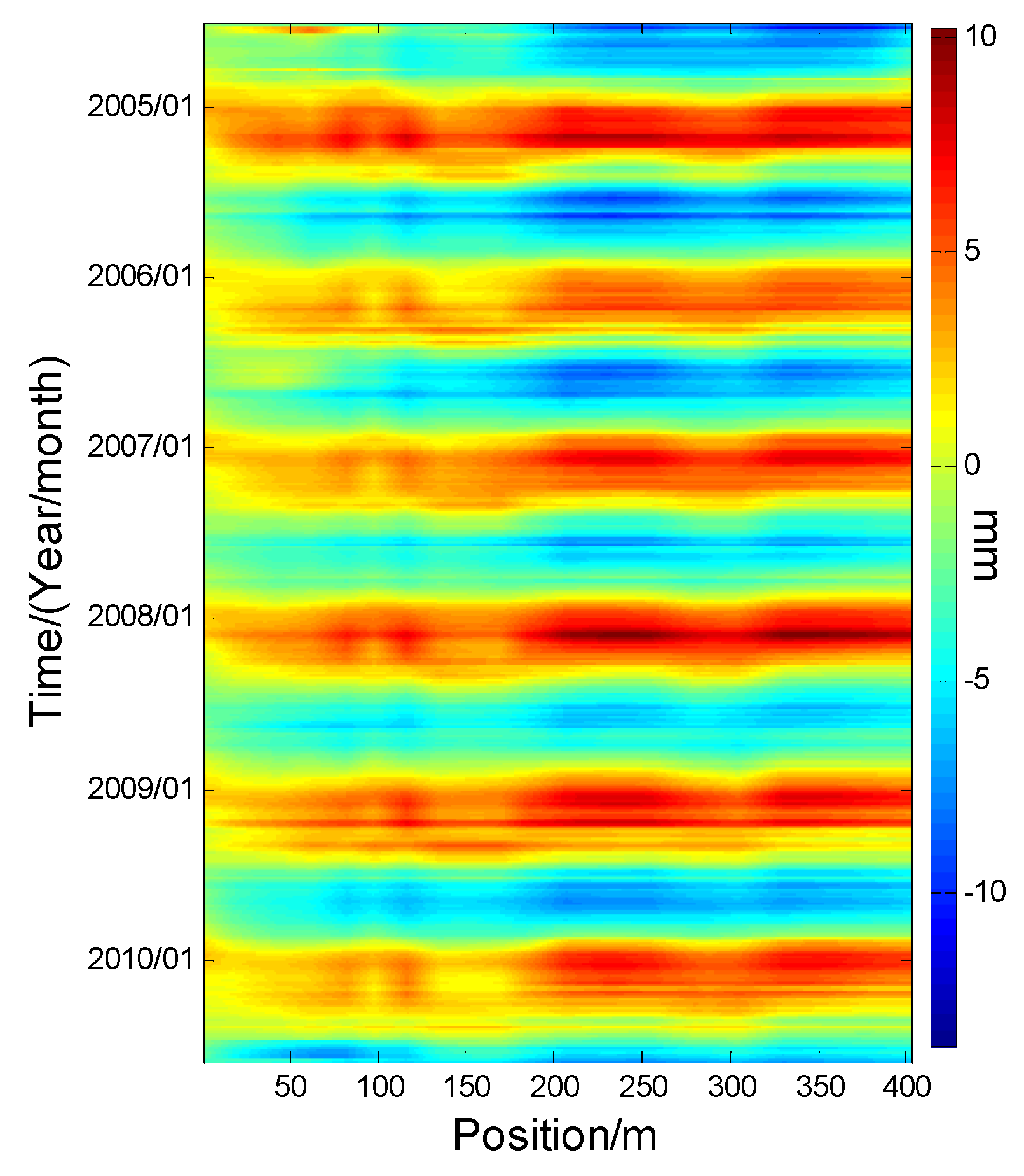
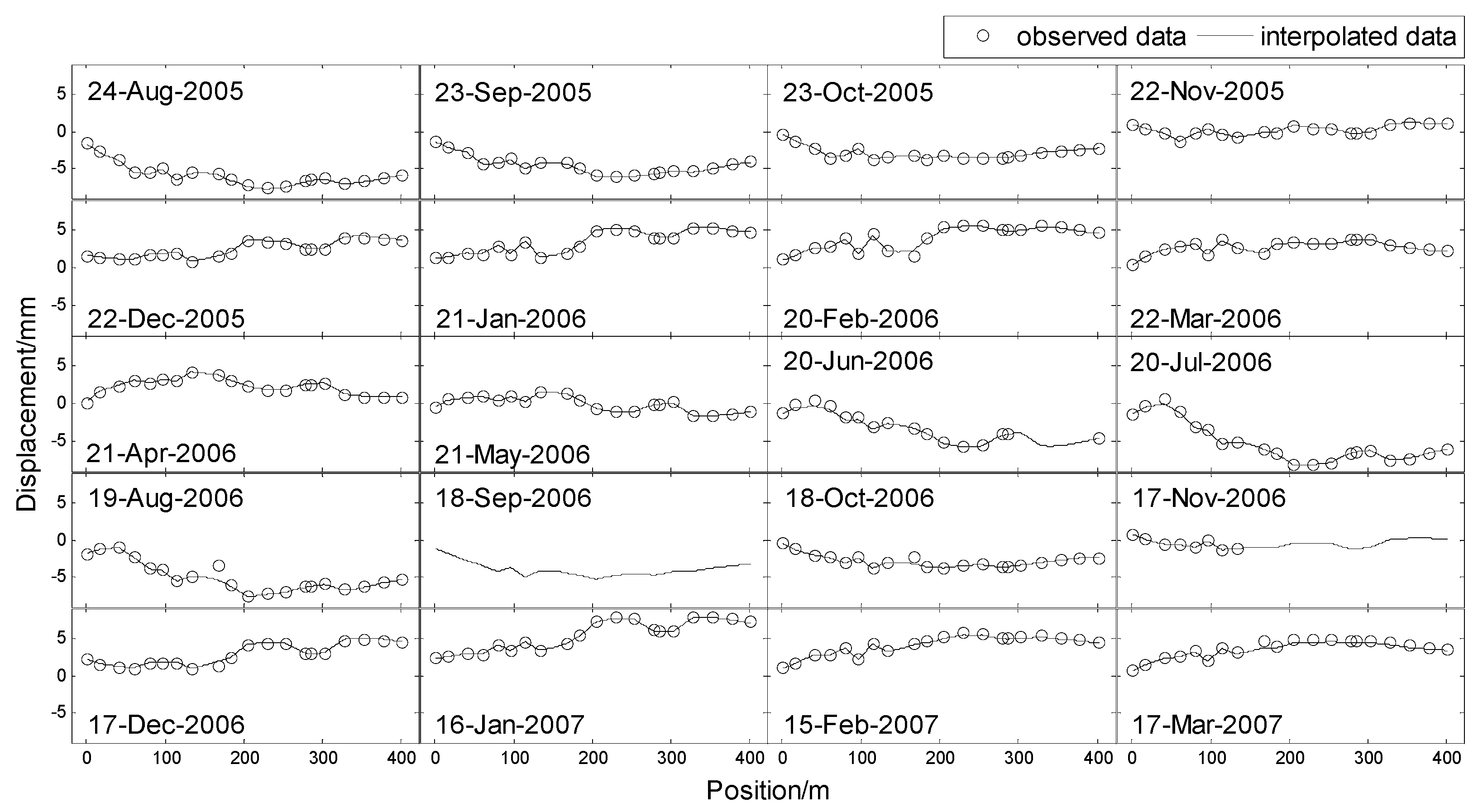
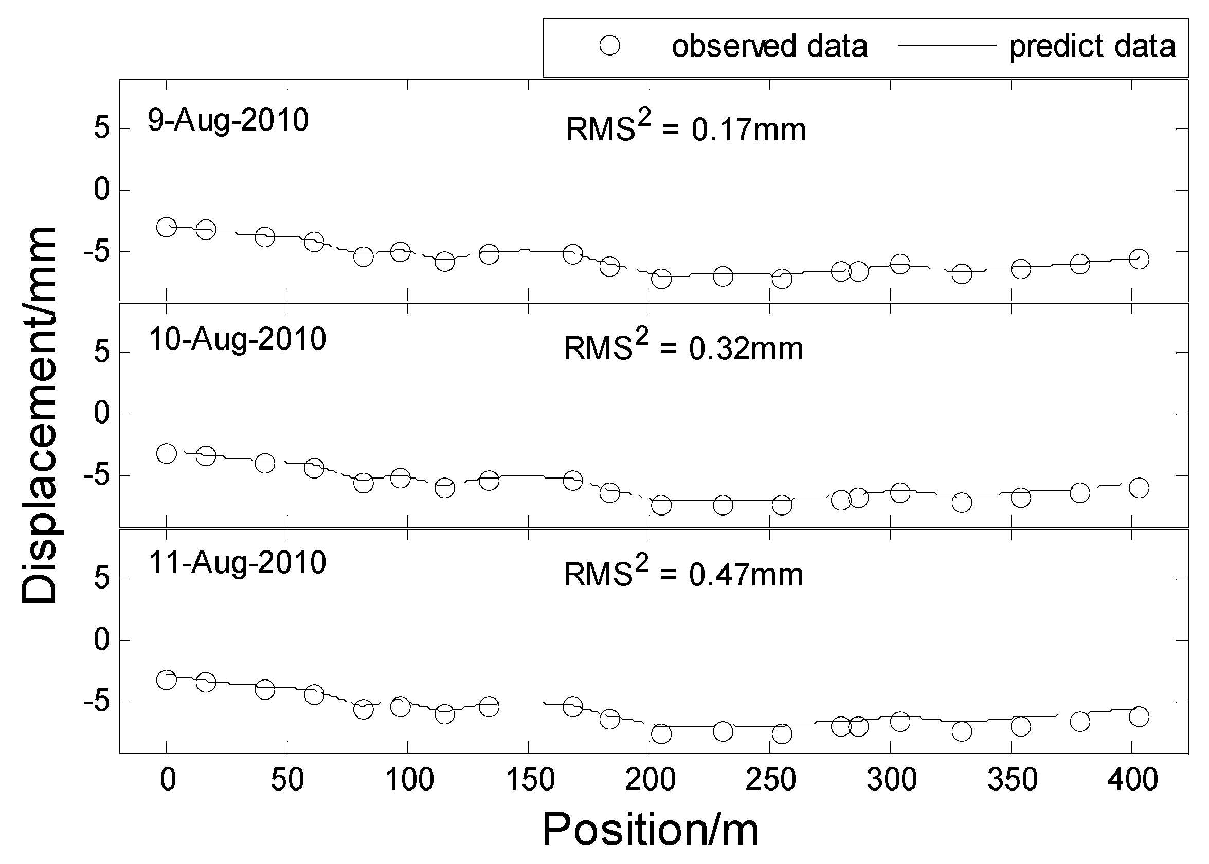
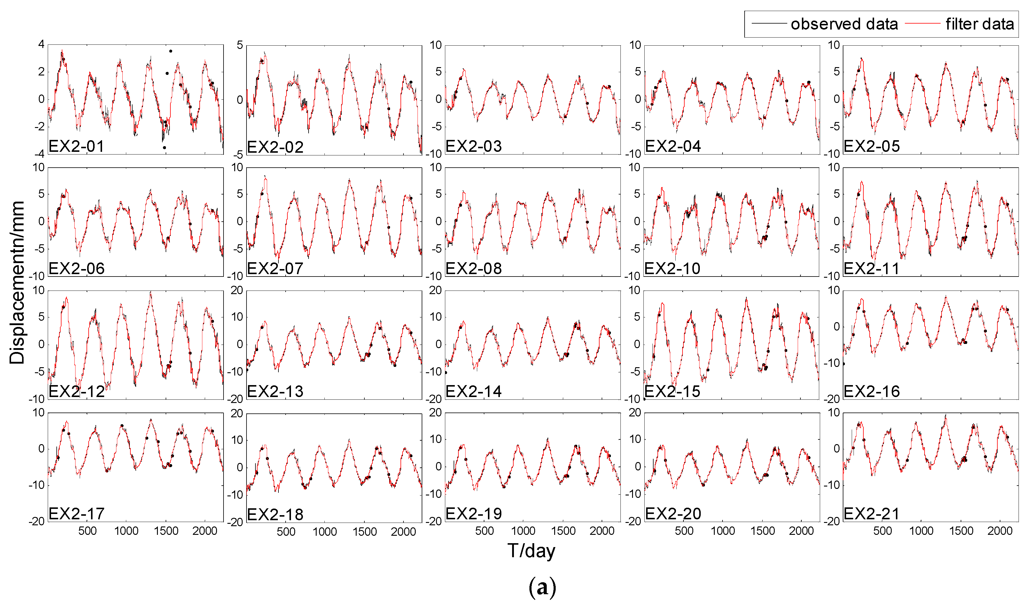
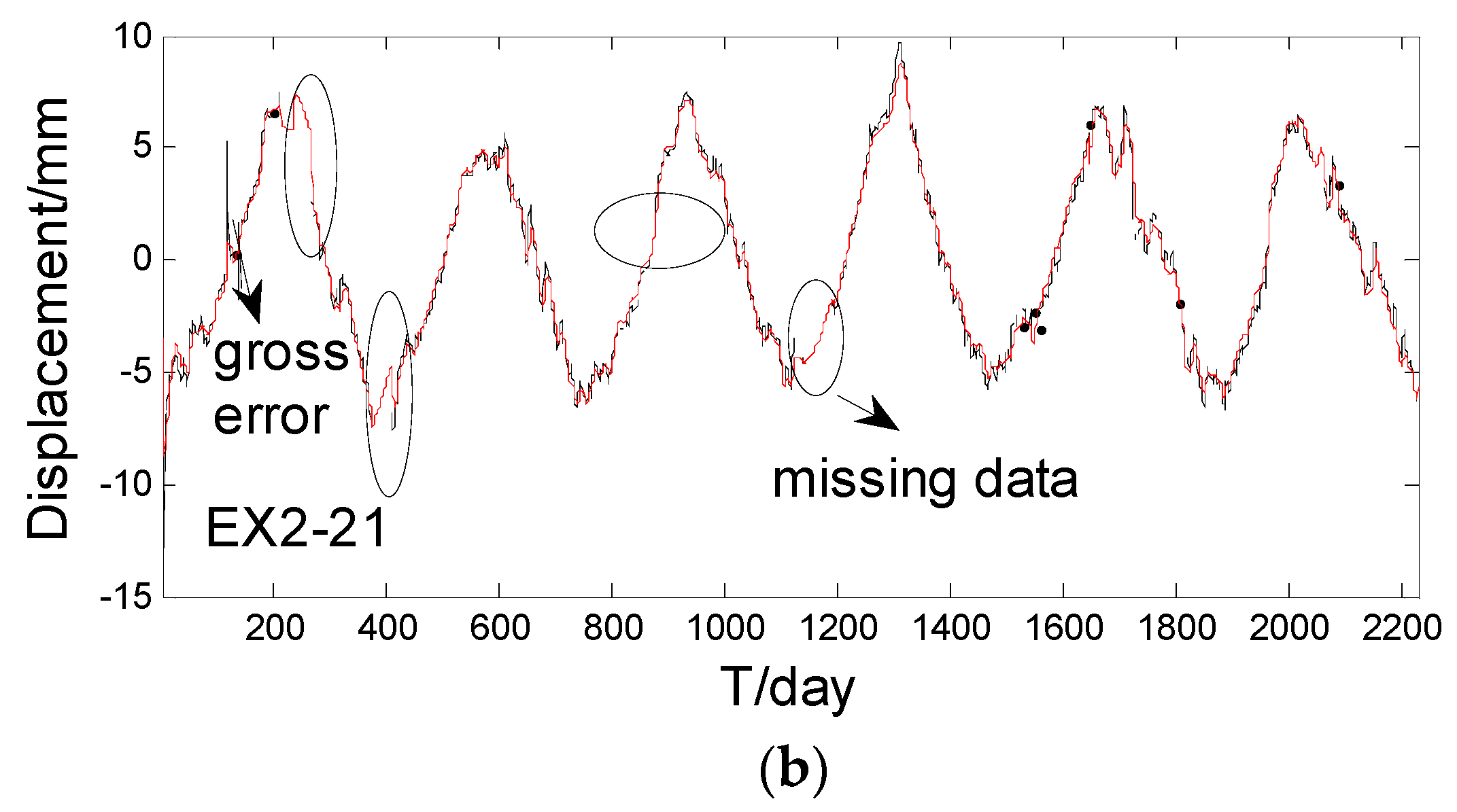
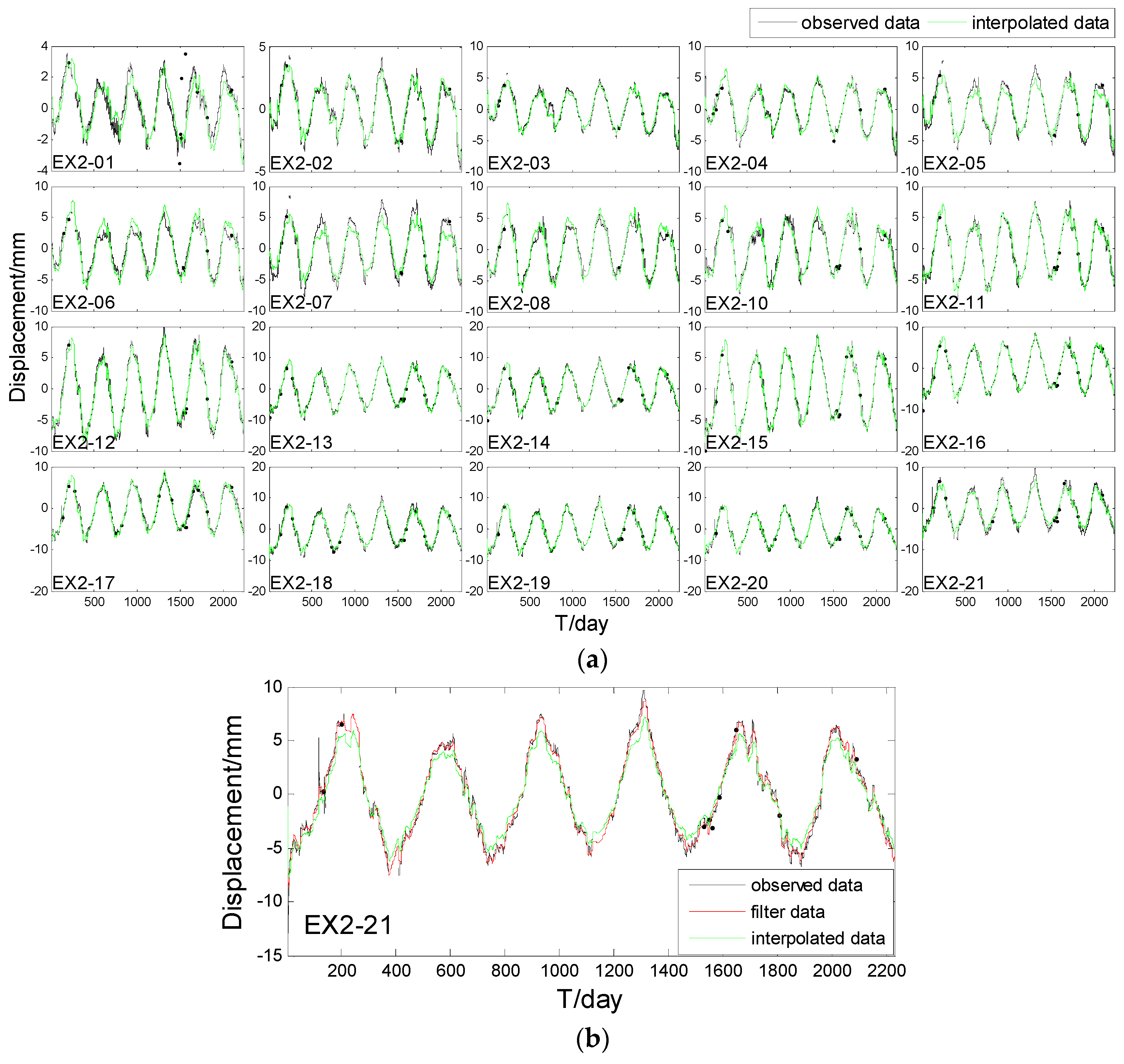
4.2. Filtering, Spatiotemporal Interpolation, and Prediction

In this experiment, displacement data before 8 August 2010 were used for filtering and interpolation. Displacement data from 9–11 August 2010 were used to verify the prediction effectiveness. Similar to the simulation experiment, we used the STKF to filter the observed data firstly. Secondly, in order to check the effectiveness of spatio-temporal interpolation using STKF, we chose 19 points as observation points, and the rest point as a check point. We Repeated the process until all the points were interpolated. Thirdly, we predicted three days’ displacement of all 20 points to check the effectiveness of the spatio-temporal prediction of STKF. Lastly, the whole dam horizontal displacement in spatio-temporal domain was interpolated to view its spatio-temporal variation, and the three days of horizontal displacement prediction for the whole dam was also included. According to the flow diagram of STKF, we randomly chose data from the 700th, 1300th, and 1600th day of dam horizontal displacement in the analysis to select space trend firstly.

Figure 5 shows that the horizontal displacement data had a linear trend, so the chosen trend matrix was $F=\left[s,1\right]$. Similar to the simulation experiment, a spherical semi-variogram model was also chosen to describe the local spatial variation. As the parameter $\theta$ of STKF was fixed, spatio-temporal filtering series, spatio-temporal interpolated series, and spatio-temporal prediction values could be obtained by implementing the STKF recursion part in Section 2.4. Figure 6a plots filtered time-series of all points and the EX2_21 point’s filtering result is enlarged in Figure 6b. Figure 7a shows interpolated time-series of all points and the EX2_21 point’s interpolated result is enlarged in Figure 7b. For the purpose of comparing the filtering result and the interpolated result, EX2_21 point’s filtering result is also displayed in Figure 7b.

Table 3. $RM{S}^2$ Filter, Interpolation, and Prediction of each point (unit: mm). Interp, Interpolation; Pred, Prediction.

Site	Filter	Pred	Interp	Site	Filter	Pred	Interp
EX2_1	0.05	0.43	0.45	EX2_12	0.16	1.07	0.52
EX2_2	0.05	0.09	0.15	EX2_13	0.18	1.07	0.32
EX2_3	0.08	0.43	0.29	EX2_14	0.18	1.14	0.45
EX2_4	0.12	0.38	0.41	EX2_15	0.12	1.06	0.2
EX2_5	0.11	0.91	0.84	EX2_16	0.12	1.05	0.19
EX2_6	0.11	0.31	1.12	EX2_17	0.12	0.31	0.53
EX2_7	0.11	0.84	1.67	EX2_18	0.2	0.70	0.74
EX2_8	0.09	0.44	0.76	EX2_19	0.22	0.58	0.4
EX2_10	0.15	0.66	0.66	EX2_20	0.23	0.41	0.42
EX2_11	0.12	0.93	0.28	EX2_21	0.21	0.53	0.92

shows statistic results of filtering, interpolation, and prediction. The statistic model of $RM{S}^2$ is as follows:

$$RM{S}^2=\sqrt{{\displaystyle \sum }_{i=1}^N{({\widehat{Y}}_i-O_i)}^2/N}$$

(26)

where ${\widehat{Y}}_i$ is the estimated value, $O_i$ is the observed value, and $N$ is the number of ${\widehat{Y}}_i$.

As Figure 6 shows, the STKF is fairly reliable in filtering the observation points. The result not only reduces the observation error of the series, but also maintains the detailed altitude change. There are big jumps on the 100th day, as shown in Figure 6b, which may have been caused by some instrumental malfunctions on that day. We consider these as gross errors and STKF can reduce their effects significantly. Ellipse in Figure 6b shows the interpolated missing data by spatio-temporal interpolation. The interpolated missing data results can connect with the filter results very well, so we can conclude that the STKF is a suitable method to interpolate the missing data.

In Figure 7a, the interpolated time-series plot coincides with the original time-series plot except for some points with peak values, such as EX2-05, EX2-06, EX2-07, EX2-08, and EX2-21. In Figure 7b, there is a small difference between the results of the 200th day, 800th day, and 1300th day. However, in EX2-11, EX2-12, EX2-13, EX2-14, EX2-15, and so on, the interpolated results perform very well even for the peak values. A possible reason of this fact could be that the chosen trend matrix is not very accurate, and the semi-variogram model cannot describe all the residual spatial variations. From Table 3, we can see that the filter $RM{S}^2$, interpolation $RM{S}^2$, and prediction $RM{S}^2$ are about 0.1 mm, 0.5 mm and 0.8 mm, respectively. The largest prediction $RM{S}^2$ is up to 1.14 mm in EX2_14, which suggests that the STKF model still has a high prediction accuracy. The larger interpolation $RM{S}^2$ occurs in EX2_6 and EX2_7, which is up to 1.12 mm and 1.67 mm, due to the slightly poor performance in peak values.

After verifying the effectiveness of spatio-temporal interpolation and prediction based STKF, the whole dam deformation in spatio-temporal domain can be interpolated and a short-term spatio-temporal prediction for the whole dam can also be predicted. Figure 8 shows interpolated horizontal displacement of the whole dam in the spatio-temporal domain. We equally chose 20 days of interpolated displacement results of the whole dam between the 420th (24 August 2005) day and the 1000th (17 March 2007) day to view the spatio-temporal variation, which is shown in Figure 9. Figure 10 shows the 3 days of prediction results for the whole dam horizontal displacement.

In Figure 8 and Figure 9, the horizontal displacement of the dam shows ‘ascend-descend’ periodic variation in the time domain. Some missing data appears on days 20 June 2006 and 17 November 2006, and all data on day 16 September 2006 is completely missed. There is an interesting phenomenon in that the interpolated results for the missing area are repeatedly similar to the results of the same area in the next subfigure. For example, the missing data interpolation results of 20 June 2006 and 18 September 2006 are very similar to that of 20 July 2006 and 18 September 2006, respectively. This indicates that the interpolated result is not only affected by its surrounding measuring points in the spatial domain, but also by its surrounding data in the temporal domain. In Figure 10, the short-term prediction result agrees with the original data, but its statistic result of the $RM{S}^2$ model seems to be larger along with the length of the backward prediction. This suggests that the prediction result may be inaccurate for long-term prediction.

5. Conclusions

This paper applied the STKF model, which combines Kalman filter and Kriging model, to analyze dam deformation data. All points are processed together, and the dam deformation is analyzed as a whole. From the experiments with simulation data and Wuqiangxi Dam tension wire data, we can infer that STKF not only can filter the deformation data noise and predict the deformation of the points effectively both in the temporal domain and spatial domain, but it can also interpolate missing data or date for any position of the dam no matter where the monitoring point is located, which cannot be achieved by the single point Kalman Filter method, because it does not consider the spatial correlation.

References

1. Wu, Z.R. Introduction. In Safety Monitoring Theory & Its Application of Hydraulic Structures; Higher Education Press: Beijing, China, 2003; pp. 1–2. (In Chinese) [Google Scholar]
2. Ince, C.D.; Sahin, M. Real-time deformation monitoring with GPS and Kalman Filter. Earth Planets Space 2000, 52, 837–840. [Google Scholar] [CrossRef]
3. Wang, Q.; Sun, H.; Li, W.; Wang, X. Application of Kalman filter analysis method in the deformation monitoring data procession. Chin. J. Eng. Geophys. 2009, 6, 658–661. [Google Scholar]
4. Li, L.; Kuhlmann, H. Real-time deformation measurements using time series of GPS coordinates processed by Kalman filter with shaping filter. Surv. Rev. 2012, 44, 189–197. [Google Scholar] [CrossRef]
5. Yang, Y.X.; He, H.B.; Xu, G.C. Adaptively robust filtering for kinematic geodetic positioning. J. Geodesy 2001, 75, 109–116. [Google Scholar] [CrossRef]
6. Kuhlmann, H. Kalman-filtering with coloured measurement noise for deformation analysis. In Proceedings of 11th FIG Symposium on Deformation Measurements, Santorini, Greece, 25–28 May 2003.
7. Szostak-Chrzanowski, A.; Chrzanowski, A.; Massiéra, M. Use of deformation monitoring results in solving geomechanical problems—Case studies. Eng. Geol. 2005, 79, 3–12. [Google Scholar] [CrossRef]
8. Dai, W.J.; Liu, B.; Meng, X.X.; Huang, D.W. Spatio-temporal modelling of dam deformation using independent component analysis. Surv. Rev. 2014, 46, 437–443. [Google Scholar] [CrossRef]
9. Cressie, N. Comment on ‘An approach to statistical spatial-temporal modeling of meteorological fields’ by MS Handcock and JR Wallis. J. Am. Stat. Assoc. 1994, 89, 379–382. [Google Scholar]
10. Huang, H.C.; Cressie, N. Spatio-temporal prediction of snow water equivalent using the Kalman filter. Comput. Stat. Data Anal. 1996, 22, 159–175. [Google Scholar] [CrossRef]
11. Goodall, C.; Mardia, K.V. Challenges in multivariate spatio-temporal modeling. In Proceedings of the XVIIth International Biometric Conference, Hamilton, ON, Canada, 8–12 August 1994.
12. Mardia, K.V.; Goodall, C.; Redfern, E.J.; Alonso, F.J. The Kriged Kalman filter. Test 1998, 7, 217–282. [Google Scholar] [CrossRef]
13. Wikle, C.K.; Cressie, N. A dimension-reduced approach to space-time Kalman filtering. Biometrika 1999, 86, 815–829. [Google Scholar] [CrossRef]
14. Cressie, N.; Wikle, C.K. Space-time Kalman filter. In Encyclopedia of Environmetrics; El-Shaarawi, A.H., Piegorsch, W.W., Eds.; John Wiley & Sons: New York, NY, USA, 2002; Volume 4, pp. 2045–2049. [Google Scholar]
15. Cortés, J. Distributed Kriged Kalman filter for spatial estimation. IEEE Trans. Auto. Control 2009, 54, 2816–2827. [Google Scholar] [CrossRef]
16. Sahu, S.K.; Mardia, K.V. A Bayesian kriged Kalman model for short-term forecasting of air pollution levels. J. R. Stat. Soc. C 2005, 54, 223–244. [Google Scholar] [CrossRef]
17. Lasinio, G.J.; Sahu, S.K.; Mardia, K.V. Modeling rainfall data using a Bayesian Kriged-Kalman model. In Bayesian Statistics and Its Applications; Upadhy, S.K., Singh, U., Dey, D.K., Eds.; Anshan: Tunbridge Wells, UK, 2006. [Google Scholar]
18. Al-Awadhi, F.A.; Alhajraf, A. Prediction of non-methane hydrocarbons in Kuwait using regression and Bayesian Kriged Kalman model. Env. Ecol. Stat. 2012, 19, 393–412. [Google Scholar] [CrossRef]
19. Qing, X.Y.; Yang, F.W.; Wang, X.Y. Short-term wind speed forecasting for multiple wind farms using Bayesian Kriged-Kalman mode. Proc. Chin. Soc. Electr. Eng. 2012, 32, 107–114. [Google Scholar]
20. Cressie, N. Spatial Prediction and Kriging. In Statistics for Spatial Data, 1st ed.; John Wiley & Sons: New York, NY, USA, 1993; pp. 105–210. [Google Scholar]
21. Sherman, M. Geostatistics. In Spatial Statistics and Spatio-Temporal Data: Covariance Functions and Directional Properties, 1st ed.; John Wiley & Sons: New York, NY, USA, 2011; pp. 21–44. [Google Scholar]
22. Bookstein, F.L. Principal warps: Thin-plate splines and the decomposition of deformations. IEEE Trans. Patt. Anal. 1989, 11, 567–585. [Google Scholar] [CrossRef]
23. Shumway, R.H.; Stoffer, D.S. An approach to time series smoothing and forecasting using the EM algorithm. J. Time Ser. Anal. 1982, 3, 253–264. [Google Scholar] [CrossRef]
24. Oliver, M.A.; Webster, R. A tutorial guide to geostatistics: Computing and modelling variograms and kriging. Catena 2014, 113, 56–69. [Google Scholar] [CrossRef]
25. Dai, W.J.; Huang, D.W.; Liu, B. A phase space reconstruction based single channel ICA algorithm and its application in dam deformation analysis. Surv. Rev. 2015, 47, 387–396. [Google Scholar] [CrossRef]
Figure 1. Flow diagram of the overall procedure of Space-Time Kalman Filter (STKF). EM algorithm, Expectation Maximization algorithm.
Ijgi 05 00236 g001
Figure 2. Interpolation of the 23 points.
Ijgi 05 00236 g002
Figure 3. Location of the tension wire measuring points. The red points in the upper part show EX2 tension wire alignment measurement points; red points in the lower part show EX1 tension wire alignment measurement points; blue points are the inverted plumb measurement points.
Ijgi 05 00236 g003
Figure 4. Displacement sequences. (a) Displacement sequence of the 20 points; (b) Displacement sequence of EX2_21.
Ijgi 05 00236 g004
Figure 5. Displacement data on the 700th, 1300th, and 1600th day.
Ijgi 05 00236 g005
Figure 6. Filter and interpolated missing data results. (a) Filter and interpolated missing data results of all points; (b) Filter and interpolated missing data results of EX2_21.
Ijgi 05 00236 g006aIjgi 05 00236 g006b
Figure 7. Interpolated time series. (a) Interpolation of all points; (b) Filter and interpolation results of EX2_21.
Ijgi 05 00236 g007
Figure 8. Interpolated horizontal displacement for the whole dam in the spatio-temporal domain.
Ijgi 05 00236 g008
Figure 9. Equally chosen 20 days of interpolated horizontal displacement for the whole dam in the spatio-temporal domain between 24 August 2005 and 17 March 2007.
Ijgi 05 00236 g009
Figure 10. Three days of horizontal displacement prediction for the whole dam.
Ijgi 05 00236 g010