Geospatial Analysis of the Building Heat Demand and Distribution Losses in a District Heating Network

Abstract

The district heating (DH) demand of various systems has been simulated in several studies. Most studies focus on the temporal aspects rather than the spatial component. In this study, the DH demand for a medium-sized DH network in a city in southern Germany is simulated and analyzed in a spatially explicit approach. Initially, buildings are geo-located and attributes obtained from various sources including building type, ground area, and number of stories are merged. Thereafter, the annual primary energy demand for heating and domestic hot water is calculated for individual buildings. Subsequently, the energy demand is aggregated on the segment level of an existing DH network and the water flow is routed through the system. The simulation results show that the distribution losses are overall the highest at the end segments (given in percentage terms). However, centrally located pipes with a low throughflow are also simulated to have high losses. The spatial analyses are not only useful when addressing the current demand. Based on a scenario taking into account the refurbishment of buildings and a decentralization of energy production, the future demand was also addressed. Due to lower demand, the distribution losses given in percentage increase under such conditions.

1. Introduction

A district heating (DH) network allows the distribution of heat from energy producers to consumers. Traditionally a combined heat and power (CHP) plant is connected to the network. Today, however, heat from decentralized renewable energy production sources such as heat pumps, biomass, geothermal and solar thermal plants can also be fed into the system [1]. Additionally, excess heat from industrial processes may contribute to thermal energy. Given the increasing rate of renewable energy production, future DH systems have to efficiently integrate a variety of energy sources [2,3,4].

A comprehensive spatial analysis of future heat demands is crucial, when existing DH networks are expanded as well as when new networks are being planned [5,6]. Most projects and applications lack exact measurements of the heat demand. The demand can instead be simulated/estimated based on information on climate, building types, and individual building characteristics, including a building’s geometry, age, condition, and number of occupants, among others [7,8]. Ref. [9] also highlights the importance of including social characteristics of an area to improve the estimation’s accuracy of the energy demand. The output of the models is often contained in digital heat atlases like Scotland heat map (www.gov.scot/heatmap) and London heat map (www.londonheatmap.org.uk). The atlases may serve as important data sources for the purpose of energy modelling [7] and planning policies [10]. If heat-metering data are available, the simulation results can be validated. Ref. [11] obtained good results when comparing simulated heat demand values with measured ones in Augsburg, Germany. Only if the energy demand, as well as its spatial (and temporal) distribution is known/estimated, can the energy system be optimized and further analyses be conducted.

The optimization of an energy system based on renewable and sustainable sources requires elaborate calculations, and has to overcome the challenge of balancing supply and demand [12]. In [13], the optimal configuration of the district heating networks was calculated based on a simplex algorithm considering pressure losses in hydraulics, investment and operational costs. The optimizations often rely on time-series of data. There is also, however, a need for studies focusing on the spatial component in connection with the temporal dimension [4]. Some studies incorporate the data directly in a spatial approach, e.g., [14] focuses on distribution losses, as well as work related to the Geographic Information System (GIS) tools STEFaN [15] and Wärmenetz-Analyst (heat net analyzer; [16]). In the latter, Ref. [17] routes the heat demand through a DH system based on the shortest path between suppliers and users. Although a common practice within the field of navigation, this technique is not commonly applied for the routing within DH networks, as it does not take into account specific heating network properties such as fluctuating demand and supply, decentralized production, flow and throughput rates, or quickly changing weather conditions. Nevertheless, it offers the opportunity of estimating the optimal dimension of DH pipelines and identifying important nodes and edges within the network. It also enables a spatial simulation of the distribution losses.

Heat distribution losses in DH networks are influenced by several factors including pipe length, dimension, insulation, temperature difference between supply and return [18,19], difference in temperature between the hot water and the material surrounding the pipe as well as the heat demand density (i.e., the amount of heat transported through the pipe). Many of the studies focus on the pipe design, dimension, and insulation [20,21] as well as water temperature [22]. These studies rely on highly detailed data. If these data are not available—which they rarely are as they are owned by private enterprises—one has to instead rely on simpler equations for the estimation of losses, e.g., losses as a function of the annual heat demand. With a low demand, the percentage losses increase dramatically; according to [23], the energy demand density has to be at least 1.5 MWh m⁻¹ year⁻¹ in order to motivate a connection to a DH network. A spatial redistribution (decentralization) of the energy production may also lead to shorter transport distances and lower distribution losses. Another measure to improve the efficiency of the system is utilizing excess heat from industrial processes [24], which otherwise would remain unused. Regardless of which measures are taken, the spatial component has to be considered in order to improve the understanding and the modeling of the system. Hence, spatial analysis of the energy demand is crucial in order to increase the efficiency of the DH network and to estimate the potential of reducing the losses.

In this study, we address the total primary energy demand for heating and domestic hot water in an existing DH network in Sinsheim, southwestern Germany. We do not aim at a fully detailed hydraulic modeling of the flow distribution. Instead, we address the geospatial topology between objects and simulate the spatial distribution of the annual heat demand within the network. Thereafter, we route the water flow through the network in order to derive the annual throughflow and demand at each net segment. Subsequently, we estimate the annual distribution losses and create a scenario with refurbished buildings, increased used of thermal solar energy and partially decentralized energy production. The aims are: (1) raising the awareness of the geospatial topology between energy producers and consumers and (2) determining the distribution losses within the district heating network by considering a trend towards decentralized energy production and improved energy efficiency in buildings. The results are particularly relevant to studies addressing the impact an increased share of renewable energy production has on DH networks. The methodology we use could be extended with more data if available. It could also be incorporated in detailed models of flow distribution and heat losses.

2. Materials and Methods

2.1. Data: Sources and Pre-Processing

Table 1. Consulted data.

Data	Data type	Attributes	Source
Building footprints	Polygon	Number of stories, building type etc.	LGL
Building address	Address data	Detailed building types	NEXIGA
Demographic data	Address data	Nr. persons and flats per building	casaGeo
Address points	Point	Geocoding of NEXIGA and casaGeo addresses	Here
TABULA typology	Buildings typology	Total primary energy demand for heating and domestic hot water	IWU
Land use	Polygon	14 land use classes	LGL
District heating network	Lines (digitalized)	DH network and DH supply area	AVR Energie GmbH

LGL—Landesamt für Geoinformation und Landentwicklung Baden-Württemberg; IWU—Institute for Housing and Environment.

gives an overview of the data used in this study. Accurate building data are necessary to estimate the spatial distribution of the heat demand in a DH network. In this study, we used a 3D building model, provided by the Baden-Württemberg State Office for Geoinformation and State Development (LGL—Landesamt für Geoinformation und Landentwicklung Baden-Württemberg). The dataset [25] includes the building footprints, number of stories, as well as the building type, among others. The dataset had to be pre-processed prior to use. First, we determined all unheated buildings based on the building type attributes and subsequently removed them. Non-heated buildings include garages, garden houses, green houses and barns, among others. Other building types present in the data set are residential building, mixed residential- and office building, office, restaurant, factory, etc. However, the data source does not provide information on the age of the building nor does it include specific subtypes of residential buildings. These two attributes were instead obtained from a commercial data set (NEXIGA) in which individual buildings are represented as address (points). The geocoding of the NEXIGA address data was done based on address points from Here. Subsequently, the geocoded NEXIGA buildings were reclassified according to the Typology Approach for Building Stock Energy Assessment (TABULA) typology [26]. The TABULA building typologies were developed in cooperation with 13 European countries and the data are available online at http://www.building-typology.eu. Since a specific national typology exists for each country, we applied the German typology [27]. The typology classifies residential buildings according to type and age, among other parameters. The typology provides values for the total primary energy demand for heating and domestic hot water for each building type. The values are available for different levels of refurbishment. However, they give no indication of user behavior or the actual heat demand.

We also included data on the DH network and land use within the project region. The DH network was digitalized from maps provided by AVR Energie GmbH (Stand 22.12.2014, available online). The general maps show the DH network as well as the supply area. Furthermore, from the same source, we identified the buildings connected to the DH network and selected them for further analysis. Some obviously missing net segments were also added based on street data. Data on land use were available from LGL. The data set has a resolution of 1:25,000 and was prepared and reclassified according to [28]. During the pre-processing, the amount of land use and land cover classes was reduced from 46 to 14 and topology errors within the data set were corrected.

For the storage and handling of spatial data, we created a PostgreSQL/PostGIS database. In the database, buildings and building types, as well as their attributes, are stored in separate tables and can be joined over a unique primary key for each building type. Subsequently, we connected ArcMap 10.3 to the database; however, the analyses are not limited to this software. The building heat demand, as well as the routing within the DH network, were conducted according to Section 2.2, Section 2.3 and Section 2.4.

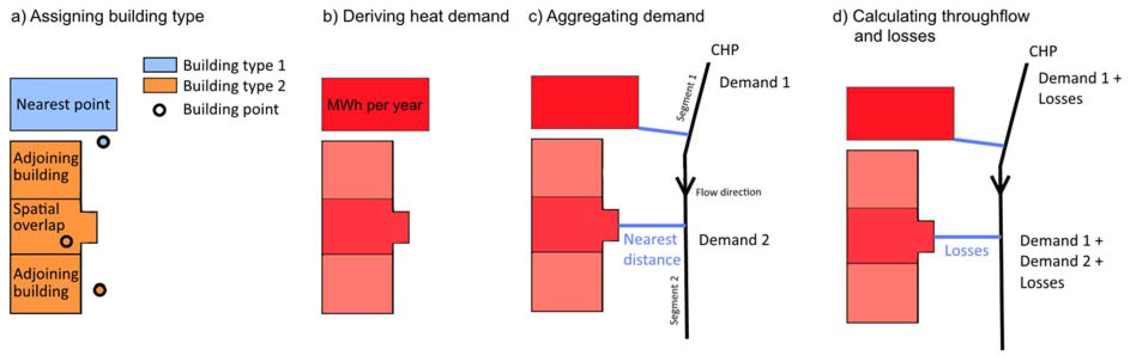
2.2. Building Heat Demand

In order to prepare a building data set, we joined the official building polygons with the established point dataset containing information regarding the TABULA type. The join was (1) first and foremost based on spatial overlaps (Figure 1a). Over 90% of the buildings could be joined based on this method. If no overlap existed, we instead assigned the same building type as the (2) adjoining building (if any). This was done by first dissolving all adjoining buildings (ArcMap tool: data management tools/generalization/dissolve). By doing this, one building type for each dissolved polygon was obtained. Thereafter, a spatial join was conducted between the original building footprints and the dissolved polygons. With this approach, each building footprint that was not initially assigned to a building type retrieved the building type information from any adjoining building. This approach also ensures that separate building parts keep their potentially different number of stories. If no adjoining buildings existed and the footprints remained unclassified, they were assigned to the same building type as the (3) closest building (geocoded NEXIGA point). This was done by first identifying the nearest point (Analysis Tools/Proximity/Near) based on the unique identifier (FID) of the buildings. Subsequently, an attributive join was conducted based on the FID. Subsequently, the buildings could be assigned to the building type of the joined (nearest) building. Building polygons, which were originally classified as a non-residential building in the official data source, were assigned to a separate building type named commercial building. This building type was not further considered within the study.

The TABULA scheme classifies residential buildings according to geographic region, year of construction, and building type, e.g., single-family house, terraced house, multi-family house or apartment block. Further information regarding building renovation could be useful for a more detailed classification. Each TABULA building type is associated with a value for the total primary energy demand for heating and domestic hot water (kWh m⁻² year⁻¹). Data are available for three building variants: existing state (no refurbishment at all), usual refurbishment and advanced refurbishment. Once we classified all buildings according to the TABULA typology, we derived the total primary energy demand for heating and domestic hot water (BuildingDemand) individually for each building according to:

BuildingDemand = Area × Stories_Nr × EnergyDemand,

(1)

where Area is the building footprint area in m² derived from the building’s polygon geometry, Stories_Nr is the number of building stories as given in the LGL data and EnergyDemand is the building-type specific total primary energy demand for heating and domestic hot water in kWh m⁻² year⁻¹ as given by the TABULA classification scheme (Figure 1b). For non-residential buildings, the TABULA classification scheme provides no information regarding heat demand. Therefore, we did not include non-residential buildings within the analysis.

2.3. District Heating Network: Routing and Losses

Once we classified the buildings according to the TABULA typology and derived their total primary energy demand for heating and domestic hot water, we analyzed the spatial variation within the DH network. First, we digitized the network and continued the analysis only with buildings connected to it. Following that, we divided the network into shorter net segments at each intersection (node). Subsequently, net segments longer than 100 m were split after 100 m in order to obtain net segments of similar length. Only end segments were allowed to be longer to avoid comparably short segments (<50 m). In the following step, we merged adjoining buildings and derived the distance from each merged building to the nearest DH network segment. The merged building thereby receives a new attribute detailing the DH network segment to which the building is connected (Figure 1c). Additionally, the distance between the building and net segment is stored. By merging buildings, we assumed that adjoining buildings have only one connection to the DH network. Thereafter, we aggregated the building heat demand according to net segments (Analysis Tools/Statistics/Summary Statistics). Then, we joined the output with the DH network layer, obtaining the annual heat demand for each net segment. In the next step, the heat demand was routed through the network.

For the purpose of routing the flow of hot water through the DH network, we built a net topology in PostgreSQL/PostGIS. The topology makes it possible to derive the shortest path between two points in the DH network, e.g., between energy providers and consumers. During the analysis, we derived the shortest path between each individual net segment and the central CHP plant. This was done with an approach similar to the one used by [17]. In this study, we conducted the routing in PostgreSQL/PostGIS by applying the Dijkstra pgrouting algorithm. Since we already obtained the annual heat demand for each DH network segment, this demand could be routed through the network and furthermore accumulated (separate R-script) at each net segment being passed through. With this approach, we obtained the amount of energy passing through (throughflow) or being consumed at this location per year (Figure 1d). As no information regarding supply and return temperature, pipe age, pipe condition or the thickness of thermal insulation were available, the distribution losses were assumed to be 25 W/m. This value can be used for new DHN with moderate supply and return temperatures [23]. We used the same value when calculating the distribution losses in the pipes connecting the buildings with the main DH network. This was done after deriving the nearest distance between the features (assumed pipe length). As already mentioned, for adjoining buildings, it was assumed that only one pipe connects with the main network.

2.4. Scenario

We created a scenario in order to simulate how refurbishment of a small percentage of buildings and an increased share of decentralized energy production influences the heat demand and losses within the DH network. For demonstration purposes, we assumed that 5% of buildings are refurbished. These buildings were randomly selected and their conditions were changed from usual refurbishment to advanced refurbishment according to the TABULA typology. According to these specifications, the buildings thereby got “equipped” with a solar-thermal system (including a daily thermal energy storage) and a ventilation system with 80% heat recovery. As a result, the total primary energy demand decreased.

Additionally, within the scenario, we assumed that 0.5 MW of the energy supplied to the system were no longer generated in the northern branch of the network. We instead assumed that this amount of energy was produced in an industrial area located in the southern branch of the network. This energy could either be supplied by biomass heating systems or originate from excess heat from industrial processes.

3. Results and Discussion

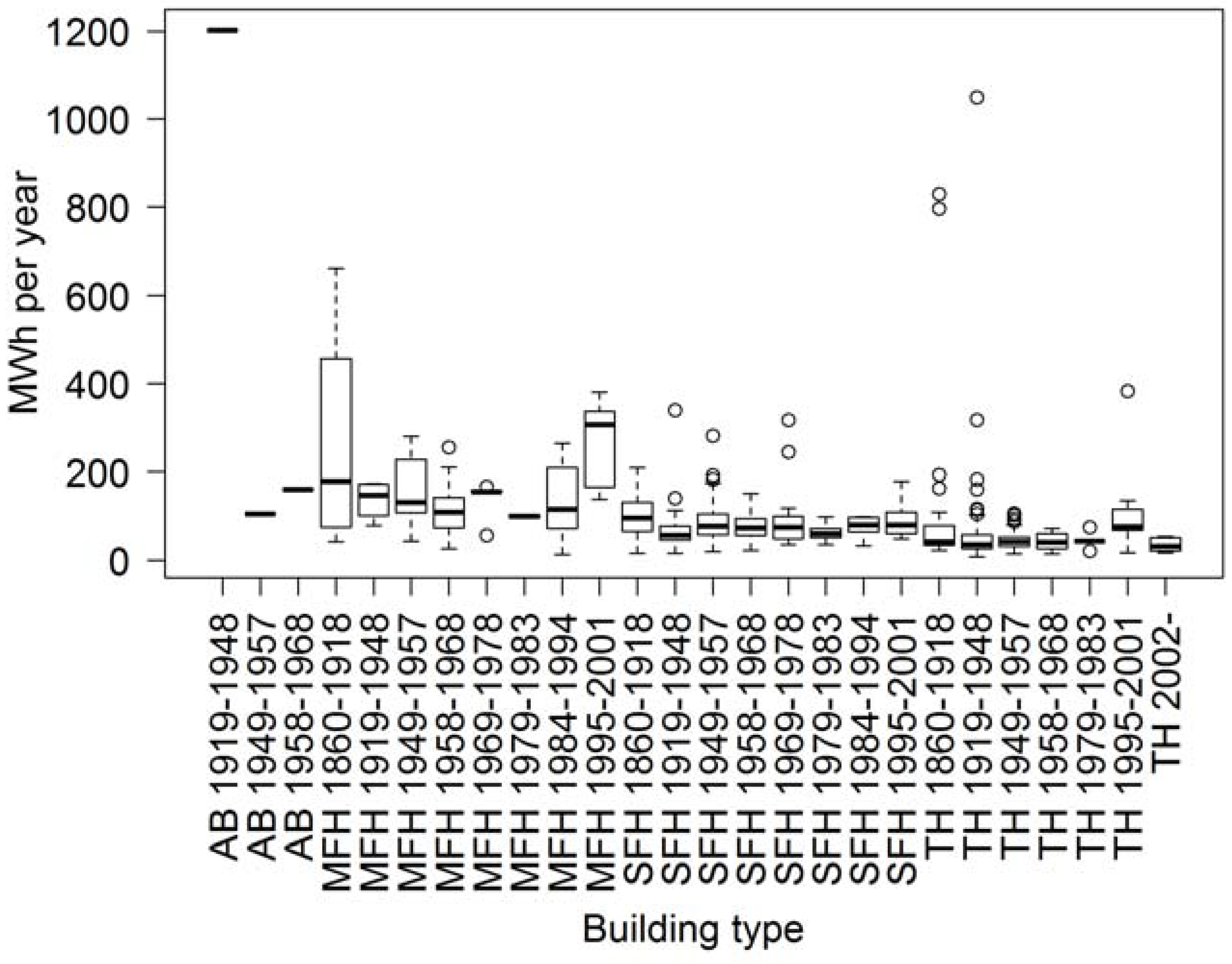
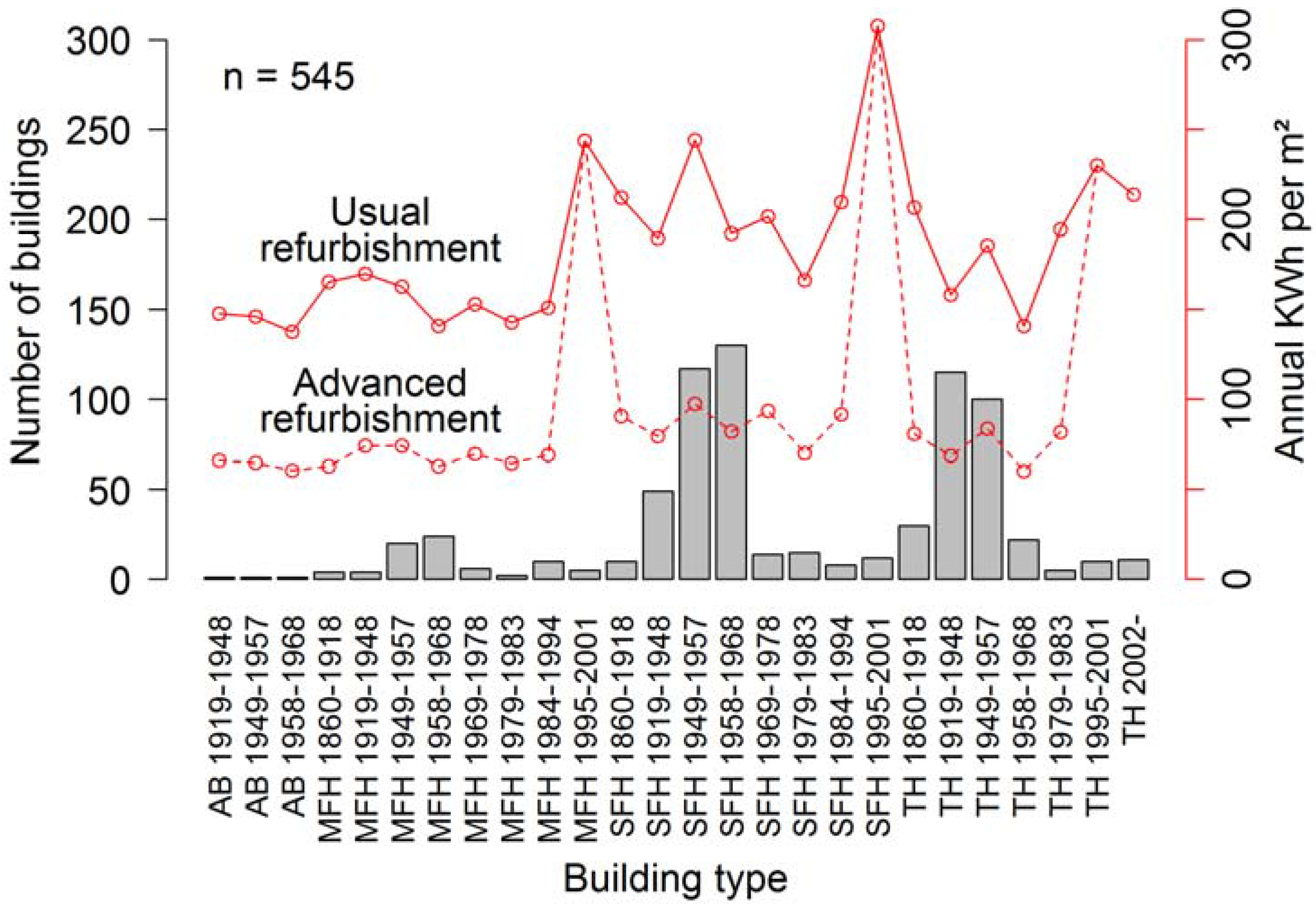
3.1. Building Statistics

Statistics of the building types show most buildings to be single-family houses (SFH) built between 1949 and 1968 (Figure 2). Terraced houses (TH) built between 1919 and 1957 are also common. The amount of multifamily houses (MFH), apartment blocks (AB) and commercial buildings (CB) is much lower. Figure 3 depicts the total primary energy demand for heating and domestic hot water given in kWh m⁻² year⁻¹. The values represent usual, as well as advanced refurbishment, and reflect a strong association between advanced refurbishment and a lower energy demand. It should be noted that, for buildings built after 2002, the only values provided describe the buildings’ existing state, since it is assumed that those buildings have not yet been refurbished. The energy demands vary significantly between buildings. The lowest demand is 13 MWh year⁻¹, whereas the highest demand is simulated to be 1202 MWh year⁻¹. The heat demand for the average building is simulated to be 99 MWh year⁻¹. The demand, furthermore, differs between building types, and the year of construction highly influences the value as well. Overall, single-family houses have the highest energy demand. Commercial buildings are not shown since no information regarding heat demand was available.

We also derived the total primary energy demand for heating and domestic hot water for individual buildings by considering the building size and number of stories (Equation (1)). The non-spatial results show that the dispersion within the building classes is high (Figure 3). This is a direct result of the great variety of building sizes within each category.

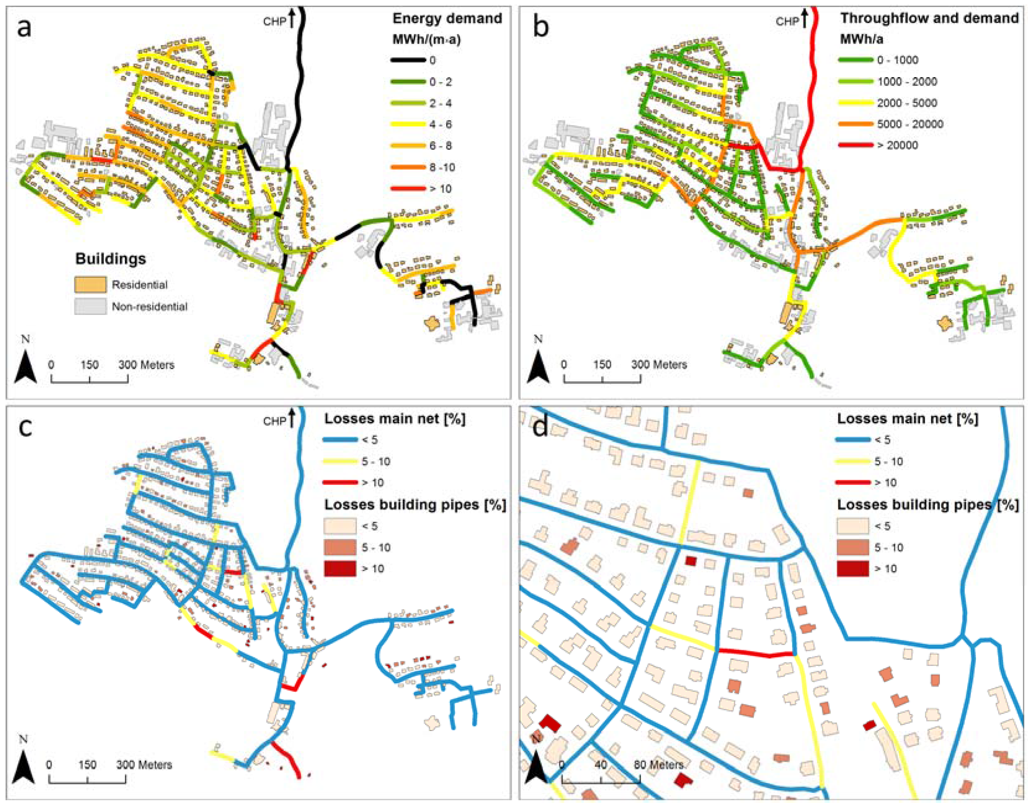
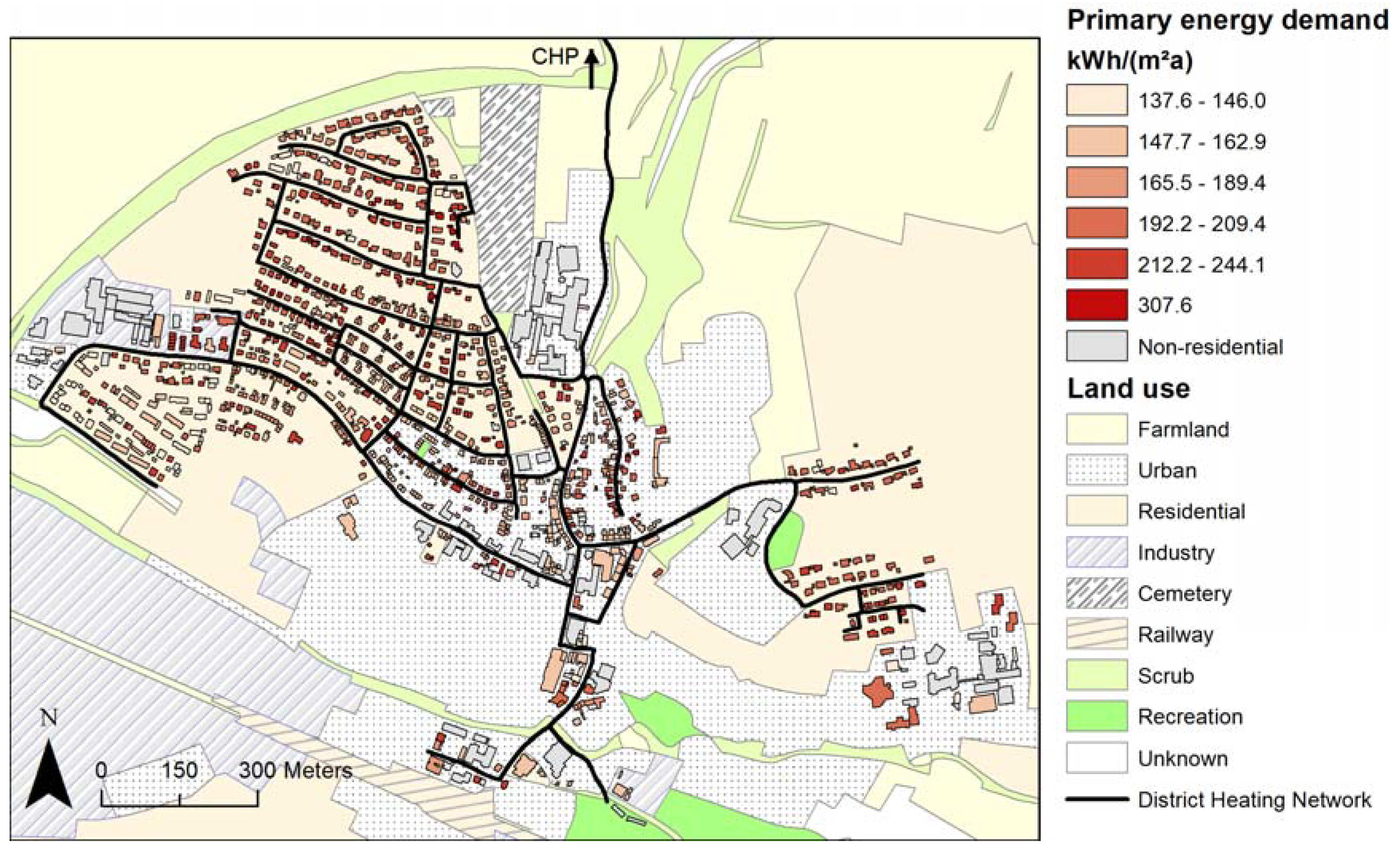
3.2. Spatial Analysis of Heat Demand and Distribution Losses

The annual total primary energy demand for heating and domestic hot water is simulated to be 54,049 MWh year⁻¹. This corresponds to a required mean production of 6.2 MW at the central CHP in order to sustain the heat demand for residential buildings. However, it should be recognized that commercial buildings are not considered. Hence, the actual production at the CHP needs to be higher. Spatial analysis of the building types and their associated energy demand indicates a heterogonous distribution of the demand within the study region (Figure 4). The results also show the buildings within residential areas to be more homogenous in size, whereas buildings within urban and industrial areas both have larger variations and show a tendency towards larger sizes.

We aggregated the energy demand according to individual DH network segments (Figure 5a). The results show how the energy demand strongly varies within the network. In relation to the building density, the demand tends to be lowest in residential areas and higher at net segments connecting urban areas. Nonetheless, also due to the mixture of building types, the smaller scaled variations are also high. Following aggregation, we routed the simulated energy demand through the DHN from the CHP to each individual net segment. Thereafter, we accumulated the values at each segment routed through and also incorporated the heat demand of the net segment itself. Compared to the heterogeneous pattern observed in Figure 5a the accumulated values show a clearer pattern depicting net segments being important for the distribution of hot water within the system (Figure 5b). As expected, the values are highest (54,049 MWh year⁻¹) at segments connected to the CHP and lowest (<1000 MWh year⁻¹) at end segments. There are also central DH network segments with low accumulated demands. These segments were simulated to have a low throughflow. This is a direct result of the model assumption. In reality, however, it may be beneficial to route the hot water differently and not simply based on the shortest distance. It may, for instance, be better to spatially apportion the throughflow of hot water more equally in order to have a smaller pipe dimension and to minimize losses. However, without further data available, the assumption of routing via shortest distance still seems realistic.

In the next step, we assessed distribution losses. Figure 5c shows the simulated losses as percentage of the accumulated demand (annual throughflow and annual demand) for the main net (164 segments). The losses associated with the pipes connecting the buildings with the main net are also shown. In the main net, the mean losses are simulated to be 2%, with values ranging from below 1% at segments with high throughflow to up to above 10% at segments with low demand and no throughflow. It shows the end segments being simulated to have the highest losses overall. It should also be noted that centrally located segments can also be associated with high losses, if no water is routed through these pipes. For the pipes connecting the buildings with the main DH network, the mean percentage loss is simulated to be 4% with values ranging from below 1% to 40%. The maximum value is a result of a stand-alone building with a long distance to the main network. In total, the losses are simulated to be 3057 MWh year⁻¹ in the main DH network (as shown in Figure 5c) and 1370 MWh year⁻¹ in the pipes connecting buildings with the main DH network. This adds up to 4427 MWh year⁻¹, which equals 8% of the total primary energy demand for heating and domestic hot water. It should, however, be emphasized that these values are purely simulated, and no data for validation are available within the study.

With this paper, our concern is to highlight the importance of the spatial aspects when simulating the district heating demand. In addition, the temporal aspects play a major role. The losses vary through the day and also between seasons. During periods and seasons with a low heat demand, the percentage losses increase. An optimal DH model should therefore include both a spatial and temporal component and preferably a more advanced formula for the calculation of losses. We are also aware of other issues that would improve the modeling, e.g., the inclusion of commercial buildings. As data were only available for residential buildings, we did not include any other buildings. This lead to an underestimation of the heat demand. Data regarding building age and usage for non-residential buildings would be valuable in order to improve the estimation of the heat demand within the DH network. Furthermore, information regarding the DH pipe dimension and insulation, etc. would permit a more detailed simulation of the losses. In real systems, point measurements of losses also contribute to valuable information for the modelling of losses for the entire systems. Nevertheless, even without these data available it is possible to demonstrate the importance of the spatial aspects when modelling DH networks.

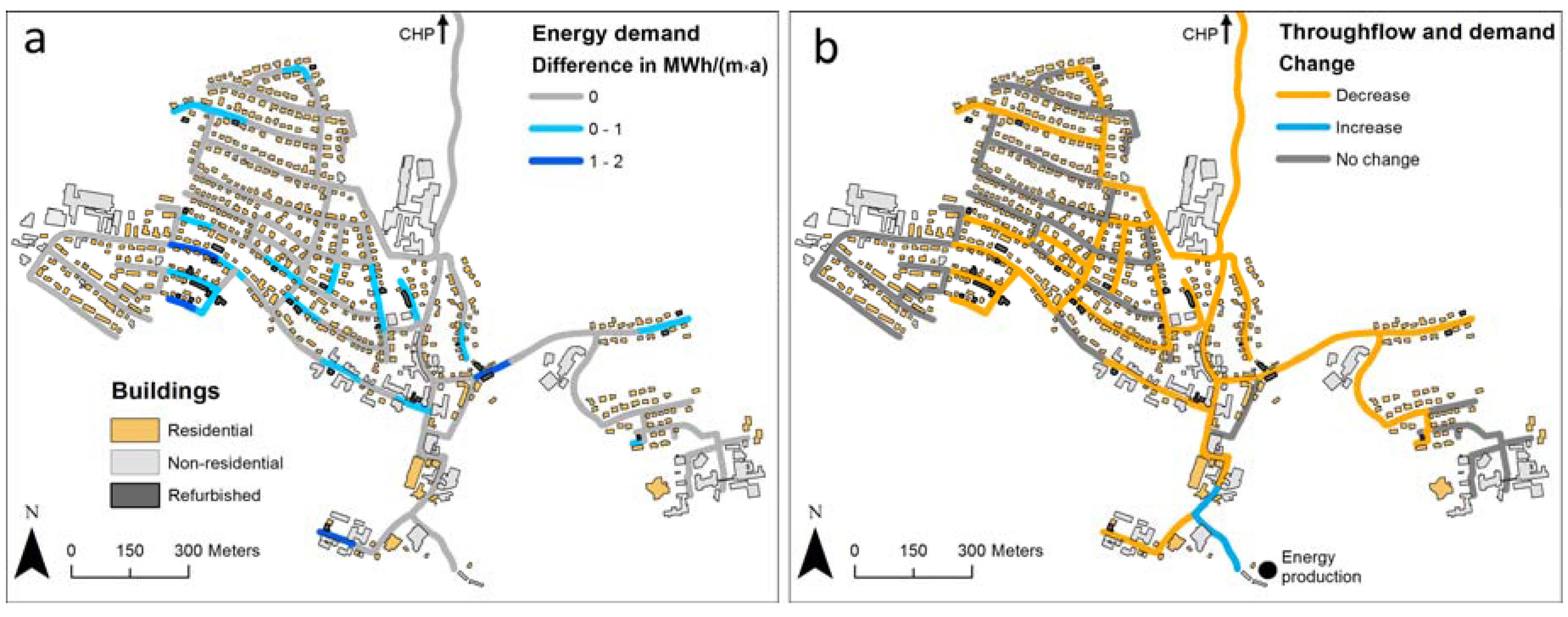
3.3. Scenario Outcome

We randomly selected 27 buildings (5% of the buildings) as being targeted for refurbishment. Furthermore, in the scenario, we assumed 0.5 MW to be generated in the southern branch of the network instead of the north. For the refurbished buildings, the heat demand decreased by 45 MWh year⁻¹ on average per building with values ranging from 13–144 MWh year⁻¹ per building. At the DH network segments where the buildings were refurbished, the demand decreased by up to more than 2 MWh m⁻¹ year⁻¹ per segment (Figure 6a). With 5% refurbished buildings, the total primary energy demand for heating and domestic hot water is simulated to be 52,819 MWh year⁻¹ for the entire system. This corresponds to a decrease of 1229 MWh year⁻¹ (reduction of 2.3% of total heat demand) in comparison to the simulated current condition. However, although we aim at estimating the energy demand as accurately as possible, it is evident that the methods are associated with several uncertainties including the fact that the current state of refurbishment remains unknown. Furthermore, the spatial distribution of the refurbished buildings influences the result. For future studies, it would also be interesting to distinguish between the impacts of different refurbishment, e.g., insulation, updated heating system, etc.

With a decreasing demand, the amount of water routed through the network decreases. According to the method used for calculating the losses, this also means that the losses increase in percentage terms. Figure 6b shows how the throughflow and the demand decrease within a majority of the network segments. Only in segments connecting the southern decentralized energy provider does the throughflow increase. The approach shows the spatial impact of improved energy efficiency of buildings and the re-distribution of supplied energy. Nonetheless, with a more advanced method for deriving the losses, these spatial characteristics could be addressed more in detail. Furthermore, the current refurbishment status and DH network properties are factors that contribute to uncertainties in the results. With more detailed data, the reliability of the results would increase.

4. Conclusions

In many European countries, the TABULA typology is useful when estimating the annual total primary energy demand for heating and domestic hot water for residential buildings. In our study region, buildings were classified according to the typology after combining data (building footprint, building type and number of stories) from several sources. Subsequently, we routed the energy demand through the DH network according to the shortest distance between energy provider and consumers. A scenario including refurbished buildings and partly decentralized energy production shows how the decreased demand has an impact on a large share of the district heating network.

Although the current refurbishment status of the buildings remains unknown, the applied approach offers the possibility of spatially simulating the building energy demand. Furthermore, even if more detailed information (pipe dimension, insolation, etc.) would improve the modelling of the DH distribution losses, the applied approach is highly useful when addressing the effects of increased renewable energy production within DH networks.

References

1. Lund, H.; Möller, B.; Mathiesen, B.V.; Dyrelund, A. The role of district heating in future renewable energy systems. Energy 2010, 35, 1381–1390. [Google Scholar] [CrossRef]
2. Lundström, L.; Wallin, F. Heat demand profiles of energy conservation measures in buildings and their impact on a district heating system. Appl. Energy 2016, 161, 290–299. [Google Scholar] [CrossRef]
3. Münster, M.; Morthorst, P.E.; Larsen, H.V.; Bregnbæk, L.; Werling, J.; Lindboe, H.H.; Ravn, H. The role of district heating in the future Danish energy system. Energy 2012, 48, 47–55. [Google Scholar] [CrossRef]
4. Resch, B.; Sagl, G.; Törnros, T.; Bachmaier, A.; Eggers, J.B.; Herkel, S.; Narmsara, S.; Gündra, H. GIS-based planning and modeling for renewable energy: Challenges and future research avenues. ISPRS Int. J. Geo-Inf. 2014, 3, 662–692. [Google Scholar] [CrossRef]
5. Nielsen, S.; Möller, B. GIS-Based analysis of future district heating potential in Denmark. Energy 2013, 57, 458–468. [Google Scholar] [CrossRef]
6. Gils, H.C.; Cofala, J.; Wagner, F.; Schöpp, W. GIS-based assessment of the district heating potential in the USA. Energy 2013, 58, 318–329. [Google Scholar] [CrossRef]
7. Finney, K.N.; Sharifi, V.N.; Swithenbank, J.; Nolan, A.; White, S.; Ogden, S. Developments to an existing city-wide district energy network—Part I: Identification of potential expansions using heat mapping. Energ. Conv. Manag. 2012, 62, 165–175. [Google Scholar] [CrossRef]
8. Kaden, R.; Kolbe, T. City-wide total energy demand estimation of buildings using semantic 3D city models and statistical data. In Proceedings of the ISPRS 8th 3DGeoInfo Conference & WG II/2 Workshop, Istanbul, Turkey, 27–29 November 2013.
9. Bale, C.S.E.; Bush, R.E.; Taylor, P. Spatial Mapping Tools for District Heating (DH): Helping Local Authorities Tackle Fuel Poverty; Project Report; Centre for Intergarated Energy Research, University of Leeds: Leeds, UK, 2014. [Google Scholar]
10. Greater London Authority. District Heating Manual for London; Greater London Authority: London, UK, 2013. [Google Scholar]
11. Herrmann, J. Optimierung der Städtischen Energieversorgung am Beispiel der Stadt Augsburg unter Besonderer Berücksichtigung von Wärmetransportmechanismen. Ph.D. Thesis, University of Augsburg, Augsburg, Germany, 2013. [Google Scholar]
12. Baños, R.; Manzano-Agugliaro, F.; Montoya, F.G.; Gil, C.; Alcayde, A.; Gómez, J. Optimization methods applied to renewable and sustainable energy: A review. Renew. Sustain. Energy Rev. 2011, 15, 1753–1766. [Google Scholar] [CrossRef]
13. Jamsek, M.; Dobersek, D.; Goricanec, D.; Krope, J. Determination of optimal district heating pipe network configuration. WSEAS Trans. Fluid Mech. 2010, 5, 165–174. [Google Scholar]
14. Vesterlund, M.; Sandberg, J.; Lindblom, B.; Dahl, J. Evaluation of losses in district heating system, a case study. In Proceedings of the 26th International Conference on Efficiency, Cost, Optimization, Simulation and Environmental Impact of Energy Systems, Guilin, China, 16–19 July 2013.
15. Gnüchtel, S. Netz-Optimierung für die Ausbauplanung (STEFaN—Software zur Trassen-Erschließung Fernwärme für Allgemeine Freie Nutzung) Computer Software. Available online: https://tu-dresden.de/ing/maschinenwesen/iet/gewv/forschung/forschungsprojekte/mldh/download_mldh (accessed on 15 November 2016).
16. KEA (Energy Agency of the State of Baden-Württemberg, Germany). Wärmenetz-Analyst (WNA) (Heat Net Analyzer). Available online: http://www.kea-bw.de/shop/startseite/ (accessed on 15 November 2016).
17. Miksche, M. Prototypische Umsetzung einer GIS-gestützten Nahwärmenetzkonzeption mit Netzwerkerstellung und—Analyse. Ph.D. Thesis, Karlsruhe University of Applied Sciences, Karlsruhe, Germany, 2011. [Google Scholar]
18. Benonysson, A.; Bohm, B.; Ravn, H. Operational optimization in a district heating system. Energy Converns. Manag. 2011, 36, 297–314. [Google Scholar] [CrossRef]
19. Dalla Rosa, A.; Li, H.; Svendsen, S. Method for optimal design of pipes for low-energy district heating, with focus on heat losses. Energy 2011, 36, 2407–2418. [Google Scholar] [CrossRef]
20. Çomaklı, K.; Yüksel, B.; Çomaklı, Ö. Evaluation of energy and exergy losses in district heating network. Appl. Therm. Eng. 2004, 24, 1009–1017. [Google Scholar] [CrossRef]
21. Yildirim, N.; Toksoy, M.; Gokcen, G. Piping network design of geothermal district heating systems: Case study for a University Campus. Energy 2010, 35, 3256–3262. [Google Scholar] [CrossRef]
22. Tol, H.İ.; Svendsen, S. Effects of boosting the supply temperature on pipe dimensions of low-energy district heating networks: A case study in Gladsaxe, Denmark. Energy Build. 2015, 88, 324–334. [Google Scholar] [CrossRef]
23. Nahwärmenetze und Bioenergieanlagen: Ein Beitrag zur effizienten Wärmenutzung und zum Klimaschutz. Available online: https://www.carmen-ev.de/files/festbrennstoffe/merkblatt_Nahwaermenetz_carmen_ev.pdf (accessed on 18 August 2016).
24. Ivner, J.; Broberg Viklund, S. Effect of the use of industrial excess heat in district heating on greenhouse gas emissions: A systems perspective. Resour. Con. Recy. 2015, 100, 81–87. [Google Scholar] [CrossRef]
25. AdV (Working Committee of the Surveying Authorities of the States of the Federal Republic of Germany). Documentation on the Modelling of Geoinformation of Official Surveying and Mapping (GeoInfoDok). Available online: www.adv-online.de/Publications/AFIS-ALKIS-ATKIS-Project/ (accessed on 15 November 2016).
26. Loga, T.; Diefenbach, N.; Stein, B. Typology Approach for Building Stock Energy Assessment. Main Results of the TABULA Project. Final Project Report; Institute for Housing and Environment: Darmstadt, Germany, 2012. [Google Scholar]
27. Loga, T.; Diefenbach, N.; Born, R. Deutsche Gebäudetypologie. Beispielhafte Maßnahmen zur Verbesserung der Energieeffizienz von typischen Wohngebäuden; Institute Wohnen und Umwelt: Darmstadt, Germany, 2011. [Google Scholar]
28. Dorn, H.; Törnros, T.; Zipf, A. Quality evaluation of VGI using authoritative data—A comparison with land use data in Southern Germany. ISPRS Int. J. Geo-Inf. 2015, 4, 1657–1671. [Google Scholar] [CrossRef]
Figure 1. (a) Each building polygon was assigned to a building type based on information from a point layer. The join was based on (1) spatial overlap. If no match could be identified, the polygon was assigned the same building type as the (2) adjoining building or (3) nearest building; (b) in the next step, building heat demand was derived based on the building size and building type; (c) the nearest distance from each building to a District Heating Network (DHN) segment was thereafter derived and the energy demand was aggregated according to net segment; and (d) the throughflow and demand was derived for each net segment based on the routing of water flow through the DHN. Distribution losses were also accounted for both in the main network and the pipes connecting the buildings with the DH net.
Ijgi 05 00219 g001
Figure 2. Number of buildings of the types Apartment Block (AB), Multi-Family House (MFH), Single-Family House (SFH) and Terraced House (TH). The building types are further categorized according to year of construction. The total primary energy demand for heating and domestic hot water is also shown in kWh m−2 year−1 for usual conditions as well as advanced refurbishment of the buildings.
Ijgi 05 00219 g002
Figure 3. Total primary energy demand for heating and domestic hot water (MWh year−1) for individual buildings (usual refurbishment). The boxes indicate the 25th–75th percentiles. The median and the upper and lower whiskers are also shown as well as outliers (indicated by circles).
Ijgi 05 00219 g003
Figure 4. Study region including land use, building footprints and district heating network.
Ijgi 05 00219 g004
Figure 5. (a) simulated annual total primary energy demand for heating and domestic hot water; (b) annual throughflow (accumulated demand) and annual demand derived based on the shortest path between the combined heat and power (CHP) plant and consumers; and (c,d) annual net losses given as percentage of primary energy demand.
Ijgi 05 00219 g005
Figure 6. (a) The difference in energy demand between the simulated current condition (as shown in Figure 5a) and the scenario simulations; and (b) the difference in throughflow and demand.
Ijgi 05 00219 g006