An Adaptive Density-Based Time Series Clustering Algorithm: A Case Study on Rainfall Patterns

Abstract

Current time series clustering algorithms fail to effectively mine clustering distribution characteristics of time series data without sufficient prior knowledge. Furthermore, these algorithms fail to simultaneously consider the spatial attributes, non-spatial time series attribute values, and non-spatial time series attribute trends. This paper proposes an adaptive density-based time series clustering (DTSC) algorithm that simultaneously considers the three above-mentioned attributes to relieve these limitations. In this algorithm, the Delaunay triangulation is first utilized in combination with particle swarm optimization (PSO) to adaptively obtain objects with similar spatial attributes. An improved density-based clustering strategy is then adopted to detect clusters with similar non-spatial time series attribute values and time series attribute trends. The effectiveness and efficiency of the DTSC algorithm are validated by experiments on simulated datasets and real applications. The results indicate that the proposed DTSC algorithm effectively detects time series clusters with arbitrary shapes and similar attributes and densities while considering noises.

1. Introduction

Time series data are very common in the real world and generally exhibit obvious spatial heterogeneity. Mining the spatial clustering characteristics of time series data is essential to exploring the potential distribution mechanism underlying this kind of data.

Many time series clustering methods have been proposed to realize the spatial clustering of the time series data. These methods can be categorized into the following five types based on the clustering mechanism: partitioning-based time series clustering algorithms [1,2,3], hierarchical time series clustering algorithms [4], density-based time series clustering algorithms [5,6], graph-based time series clustering algorithms [7] and time series co-clustering algorithms [8,9]. Although these algorithms can handle certain applications, they still suffer from several deficiencies and require improvement. For example, most existing algorithms cannot adaptively detect clusters because they require several predefined parameters that depend heavily on prior knowledge; however, prior knowledge is always limited in real applications. As another example, current algorithms ignore spatial heterogeneity and seldom consider spatial attributes. In real applications, many geographical phenomena, such as surface deformation, rainfall and the heavy mental content of soil, are influenced by the surrounding environment. The objects of these phenomena are generally similar with a short spatial distance. Meanwhile, if spatial attributes are neglected, clusters with similar non-spatial attributes will overlap, and objects in clusters will be dispersedly distributed in the spatial domain. This phenomenon partially violates the real conditions and affects the visualization effect. Hence, spatial attributes should be considered to correctly obtain the spatial clustering characteristics of time series data. Additionally, either the similarity of non-spatial time series attribute values or the similarity of non-spatial time series attribute trends is considered in measuring the attribute similarity between objects. However, objects with similar non-spatial time series attribute trends but significantly different non-spatial time series attribute values will be incorrectly detected as similar objects in the non-spatial domain when only the similarity of non-spatial time series attribute trends is considered in measuring the non-spatial attribute similarity. Similarly, if the non-spatial time series attribute trends between objects are significantly different and the non-spatial time series attribute values between them are similar, then the objects will also be incorrectly recognized as similar objects in the non-spatial domain if only the similarity of non-spatial time series attribute values is considered in measuring the non-spatial attribute similarity. Furthermore, time series data with similar attribute trends and different attribute values or similar attribute values and different attribute trends exist in real applications. For example, areas with monsoon climates of medium latitudes are rainy during summer and dry during winter. The rainfall trends in these areas are similar. However, the rainfall capacity depends on location. Hence, rainfall trends and rainfall capacity should be considered simultaneously to mine areas with similar rainfall. Therefore, the similarity of non-spatial time series attribute values and the similarity of non-spatial time series attribute trends should be considered simultaneously to correctly mine the clustering distribution characteristics of objects.

To overcome the above-mentioned deficiencies, a novel density-based time series clustering (DTSC) algorithm, is proposed based on a density-based spatial clustering (DBSC) algorithm [10]. The proposed DTSC algorithm can adaptively detect clusters with similar spatial attributes, non-spatial time series attribute values and non-spatial time series attribute trends. In addition, the corresponding clusters are non-overlapping for a clear visualization. More importantly, applications related to complicated time series with unequal lengths (time intervals in time series are unequal) and noises are ubiquitous. Un-equal time intervals and noises are considered in the proposed method to simulate complicated real-world applications.

The remainder of the paper is organized as follows. Section 2 briefly describes the strategy of the adaptive time series spatial clustering. The proposed algorithm is introduced and the corresponding accuracy analysis methods are discussed in Section 3. In Section 4, experiments on simulated datasets and real applications are conducted to verify the feasibility of the proposed algorithm. Finally, the results are discussed further in Section 5.

2. Methods for Time Series Clustering

Performing the adaptive time series clustering depends on two difficult aspects. One is the measurement of the similarity between time series objects, and the other involves the adaptive strategy of the time series clustering.

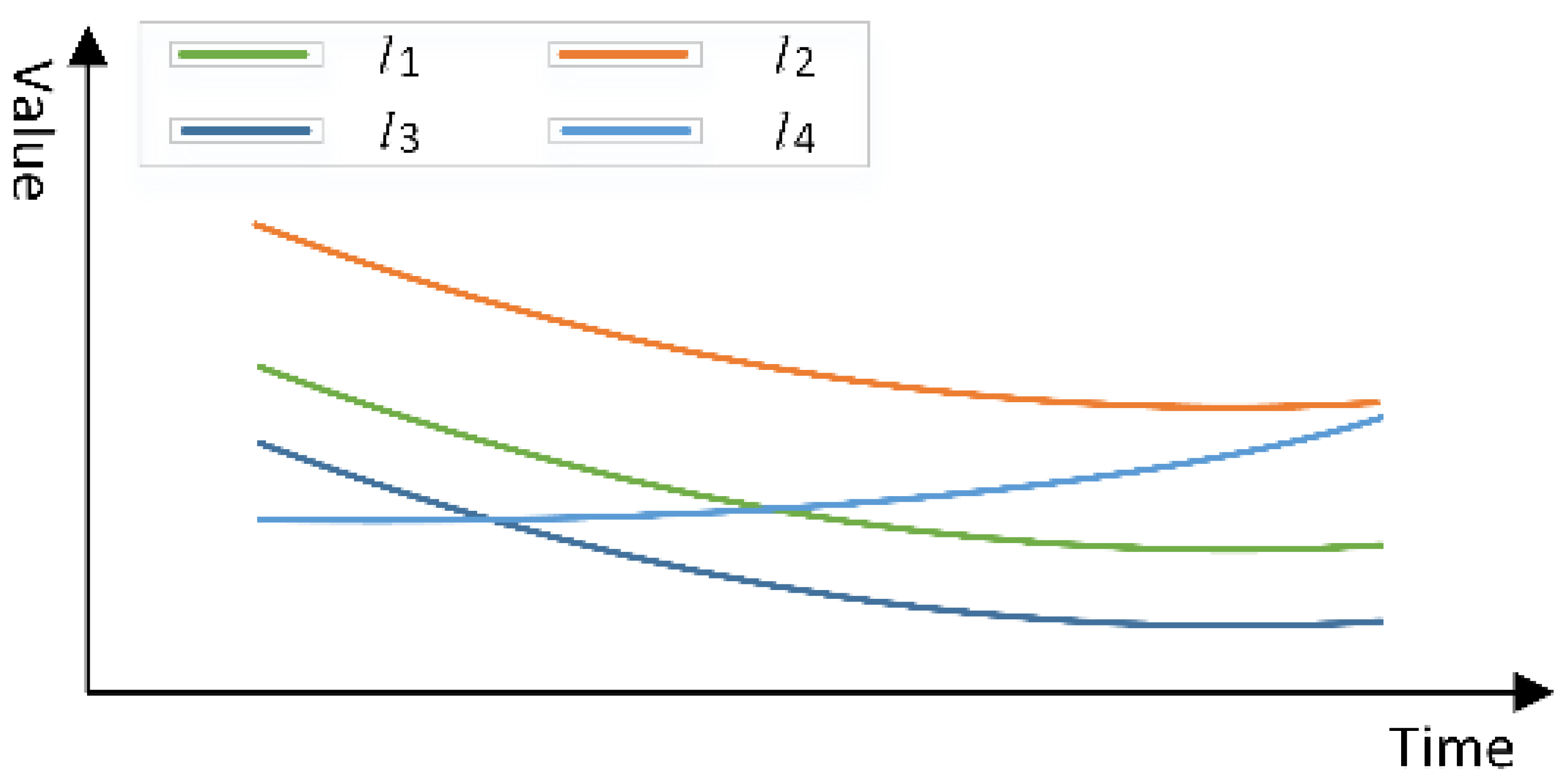
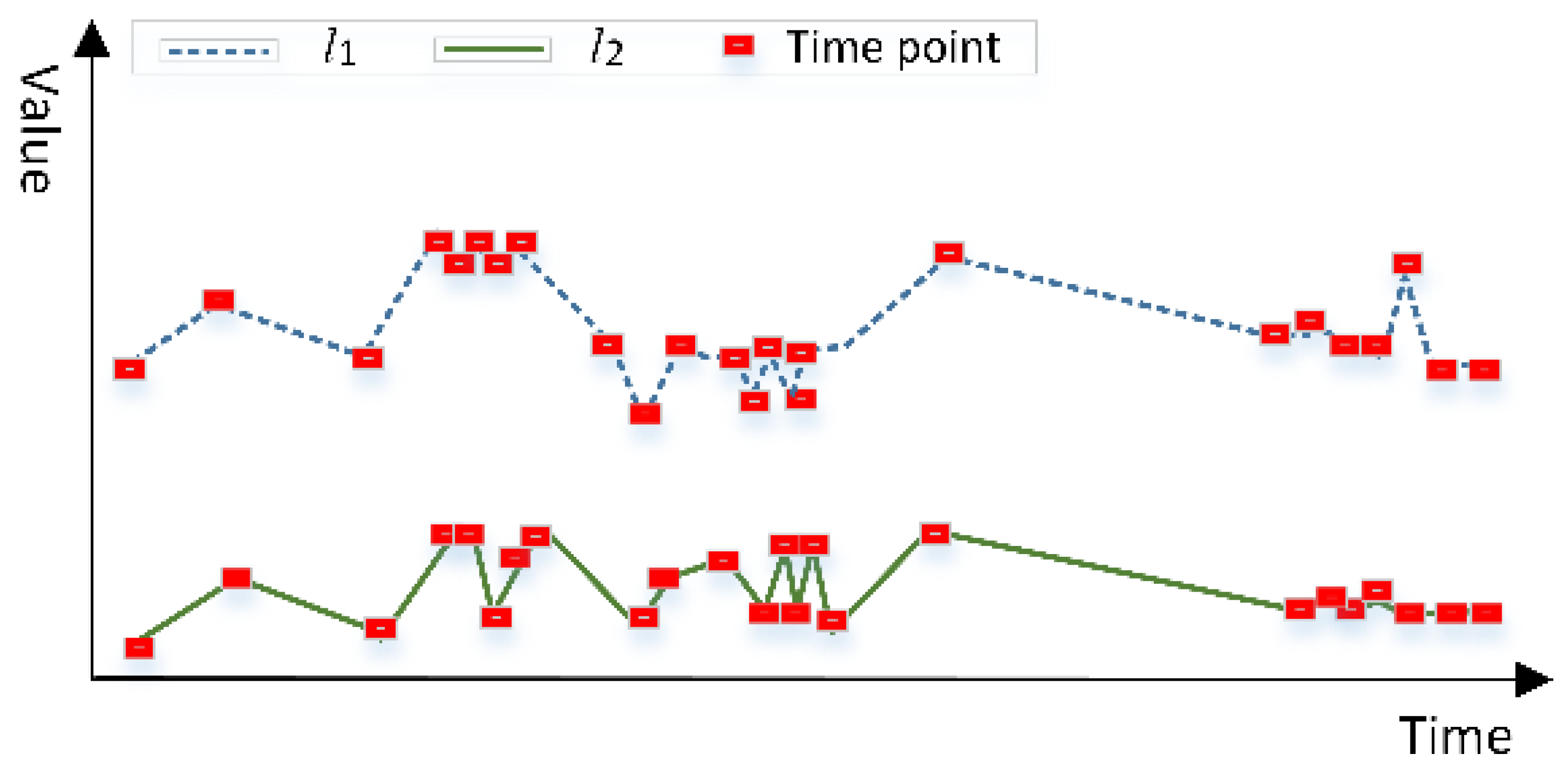
2.1. Measurement of Similarity between Objects

Spatial and non-spatial similarities are considered interdependently to eliminate the need to determine suitable weightings for the similarity between objects in the spatial and non-spatial domains. The Euclidean distance, which is useful to measure the spatial attribute similarity, is utilized for the spatial domain in this study. On the other hand, the Euclidean distance (measuring the similarity of non-spatial time series attribute values) or Pearson’s correlation coefficient (measuring the similarity of non-spatial time series attribute trends) are commonly used to measure non-spatial attribute similarities, but these methods cannot effectively separate certain phenomena, as shown in Figure 1 and Figure 2.

Figure 1 shows that the time series object $l_1$ is more similar with the object $l_3$ than with the objects $l_2$ and $l_4$. However, the Euclidean distance between objects $l_1$ and $l_3$ is equal to that between objects $l_1$ and $l_4$. The Pearson’s correlation coefficient between $l_1$ and $l_2$ is equal to that between $l_1$ and $l_3$. Using only one of the two similarity measurement methods would obviously produce an inaccurate judgment regarding the degree of similarity between the time series objects. However, if the Euclidean distance and Pearson’s correlation coefficient were utilized in combination to measure the degree of similarity between objects, then the result would show that the degree of similarity between $l_1$ and $l_3$ is the highest among all pairs. Hence, the judging criterion of the degree of similarity should be based on the Euclidean distance and Pearson’s correlation coefficient—the larger the value of the Pearson’s correlation coefficient and the smaller the value of the Euclidean distance, the higher the degree of similarity of the non-spatial attribute of the two objects will be.

In addition, the existing Euclidean distance and Pearson’s correlation coefficient ignore the un-equal time series phenomenon, as is shown in the time series objects in Figure 2. Figure 2 shows that the un-equal time interval phenomenon hinders the existing similarity measurement methods. The non-spatial attribute trend between the time series objects $l_1$ and $l_2$ are apparently similar by visualization, whereas the Pearson’s correlation coefficient between $l_1$ and $l_2$ is 0.423 with a significance level 0.029 and cannot represent the degree of similarity between time series objects with un-equal time intervals. An improved similarity measurement method that considers un-equal time series is proposed to increase the accuracy of measuring the degree of similarity of non-spatial attributes between time series objects. This method adopts a weighted Euclidean distance (Equation (1)) to measure the similarity of non-spatial attribute values and a weighted Pearson’s correlation coefficient (Equation (2)) to measure the similarity of non-spatial attribute trends. According to Ramirez-Lopez et al. [11], if the Pearson’s correlation coefficient between two time series objects is larger than 0.6 and the significance level is less than 0.1, then the time series objects represent a significantly similar attribute trend. The weighted Pearson’s correlation coefficient between $l_1$ and $l_2$ is 0.786 with a significance level 0.001, which shows that the attribute trend between $l_1$ and $l_2$ is significantly similar.

$$D\left(l_1,l_2\right)=\sqrt{{\displaystyle \sum }_{i=1}^{T}w\left(t\left(i\right)\right){\left(l_1^{t\left(i\right)}-l_2^{t\left(i\right)}\right)}^2}$$

(1)

$$pcw\left(l_1,l_2\right)=\frac{{{\displaystyle \sum }}_{i=1}^{T}w\left(t\left(i\right)\right)l_1^{t\left(i\right)}\times l_2^{t\left(i\right)}}{\sqrt{{{\displaystyle \sum }}_{i=1}^{T}w\left(t\left(i\right)\right){l_1^{t\left(i\right)}}^2}\sqrt{{{\displaystyle \sum }}_{i=1}^{T}w\left(t\left(i\right)\right){l_2^{t\left(i\right)}}^2}}$$

(2)

where $l_1^{t\left(i\right)}$ is the value in the $i\mathrm{th}$ time point of time series object $l_1$, and $w\left(t\left(i\right)\right)=\raisebox{1ex}{$\left(t\left(i\right)-t\left(i-1\right)\right)$}\!\left/ \!\raisebox{-1ex}{$\left(t\left(T\right)-t\left(0\right)\right)$}\right.$.

2.2. A New Adaptive Strategy for Time Series Clustering

A strategy of separately detecting clusters in the spatial and non-spatial domains is proposed in this study to adaptively identify the clusters with similar spatial and non-spatial attributes. The Euclidean distance is adopted in the spatial domain. Considering the neighboring relationship between objects [10], spatial proximity relationships between time series objects are adaptively obtained by removing inconsistent edges in the constructed Delaunay triangulation of objects by merging the particle swarm optimization (PSO) algorithm [12]. Then, based on the spatial proximity relationships, clusters with neighboring objects having similar non-spatial time series attributes are adaptively clustered by using an improved density-based time series clustering method in the non-spatial domain. The density based time series clustering method is improved by integrating the proposed similarity measurements (described in Section 2.1) and the strategy of density indicator of a dual density-based clustering method (DBSC) [10], to be introduced in Section 3.

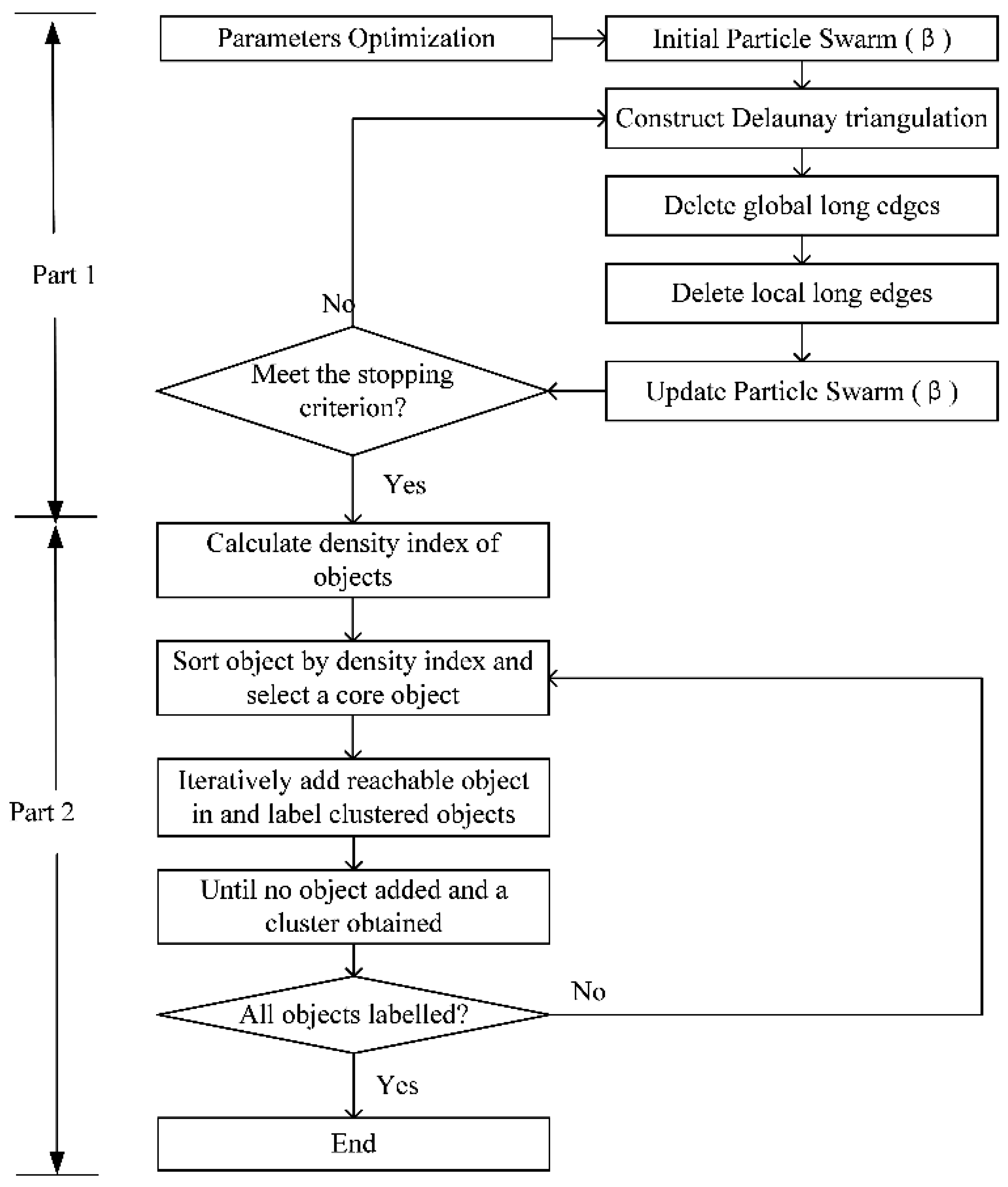
3. The DTSC Algorithm

The DTSC algorithm comprises two phases. In phase 1, spatial proximity relationships are constructed by removing the inconsistent edges that are excessively long at the global and local levels. This phase is adaptively controlled by PSO, as illustrated in Section 3.1. Phase 2 is then conducted based on the spatial proximity relationships, and an improved density based clustering method is utilized to adaptively detect clusters with similar time series attributes, which will be discussed in Section 3.2. The main procedures of DTSC are schematically shown in Figure 3. Eventually, to evaluate the result of DTSC algorithm, evaluation indexes are introduced and described in Section 3.3.

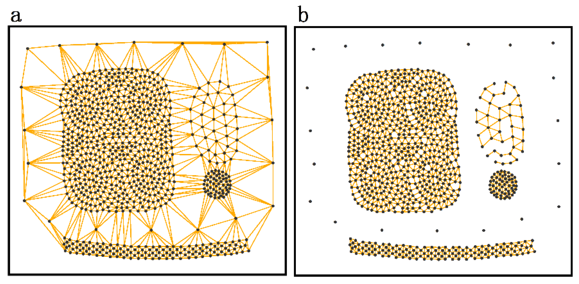
3.1. Construction of Spatial Proximity Relationships

Delaunay triangulation is a useful tool for constructing the spatial neighboring relationships [13], but there are generally some inconsistent edges in the constructed Delaunay triangulation. Hence, spatial proximity relationships are constructed by removing the inconsistent edges, which is derived from the spatial proximity construction procedure of DBSC [10]. The major steps are introduced as follows:

Step 1: The Delaunay triangulation $G$ is constructed.

Step 2: The global distance constraint is calculated by the following equation:

$$\begin{array}{l}Global\_cut\_Value\left(p_i\right)\\ =Global\_mean\left(G\right)\\ +\raisebox{1ex}{$Global\_mean\left(G\right)\times Global\_variation\left(G\right)$}\!\left/ \!\raisebox{-1ex}{$mean\left(p_i\right)$}\right.\end{array}$$

(3)

where $Global\_mean\left(G\right)$ and $Global\_variation\left(G\right)$ are the mean value and standard deviation of the length of the edges in $G$, respectively; and $mean\left(p_i\right)$ is the mean value of the length of the edges in relation to $p_i$.

Step 3: The long edges are deleted at a global level in $G$. The edge connected to $p_i$, which has distance larger than $Global\_cut\_constaint\left(p_i\right)$, should be deleted to remove the global inconsistent edges.

Step 4: The local distance constraint is calculated by the following equation:

$$Local\_cut\_value\left(p_i\right)=Mea{n}_{G_i}^2+\beta \times Mean\_variation\left(G\right)$$

(4)

where $Mea{n}_{G_i}^2$ is the mean length of the edges by the points equal to less than the second-order neighbors of $p_i$; $Mean\_variation\left(G\right)$ is the mean value of the local variation of the points in graph$G$; and $\beta$ is the adjustment parameter that controls the sensitivity of spatial attributes. In practice, $\beta$ is set from 1 to 2 [10]. The smaller the value of $\beta$ is, the easier the long edges can be deleted.

Step 5: The long edges are deleted at the local level. The edge connected to $p_i$, whose distance is larger than $Local\_cut\_value\left(p_i\right)$, should be deleted to remove local inconsistent edges. Objects connected are considered neighbors and sub-graphs with connected objects are obtained.

$\beta$ largely affects the result of the proximity relationships. Evaluation and optimization of $\beta$ are necessary and are therefore applied in this study to obtain satisfactory results under the proper value of $\beta$. The construction of proximity relationships is a graph based clustering method [14]. Hence, a graph-based evaluation function [15] that considers spatial outlier effectiveness is utilized in this phase; this method can accurately evaluate the feasibility of the spatial proximity construction results. The evaluation function is defined as follows:

$$Z=\raisebox{1ex}{$\left(P+Q\right)\times {}_{i=1,\cdots M}{}^{\min }{F}_I\left(G_i\right))$}\!\left/ \!\raisebox{-1ex}{${{\displaystyle \sum }}_{i=1}^M{F}_E\left(G_i\right)+{{\displaystyle \sum }}_{j=1}^N{F}_E\left(O_j\right)$}\right.$$

(5)

where $P$ and $Q$ are the number of clusters and noises, respectively; $Z$ is the evaluation value; $F_E\left(G_i\right)$ is the inter-graph similarity of sub-graph $G_i$; $F_E\left(O_j\right)$ is the similarity between outlier $O_j$ and sub-graphs; and $F_I\left(G_i\right)$ is the intra-cluster similarity of $G_i$.

According to the evaluation function, the value of Z will be large, if the similarity of inter-graph is high and if the similarity of intra-graph and similarity of graph and noises are low. PSO [12] is used to adaptively search for the good result with the largest $Z$ and proper $\beta$ automatically. The optimization procedure terminates until the Z value converges to a global maximum. The execution time is labeled as $k$. The time cost of the optimization procedure mainly depends on the data size and $k$. The computational efficiency of phase 1 is $O\left(k\times \left(\mathrm{Nlog}\left(\mathrm{N}\right)\right)\right)$. $k$ can be significantly decreased by a using parallel skill [16].

3.2. Clustering Objects with Similar Time Series Attributes

In the non-spatial domain, an improved time series clustering method is proposed based on the strategy of density indicator of DBSC algorithm [10]. The procedure can be divided into two parts. Part 1 calculates the degree of similarity based on the spatial proximity relationships. The degree of similarity between objects without a proximity relationship is considered to be near zero [10]. Part 2 aggregates objects with similar time series attributes. Several basic principles are first introduced to clarify the proposed method.

(1)

Spatial neighbors: Objects connected by edges in the modified Delaunay triangulation.

(2)

Attribute directly reachable: Objects with similar time series attribute values and attribute trends are considered as attribute directly reachable. The object $p_1$ and $p_2$ are attribute directly reachable, if

(i)

$pcw\left(p_1,p_2\right)>0.6$ and $sig\left(p_1,p_2\right)<0.1$; and

(ii)

$D\left(p_1,p_2\right)<TS$

where $TS$ is the threshold of the non-spatial attributes, which can be calculated as follows. First, the attribute distances $D$ between neighboring objects are calculated. Secondly, objects and minimum attribute distance objects are searched and labeled. The mean of the minimum attribute distances is calculated and assigned to$TS$. The effectiveness of this method has been experimentally proven [10].

(3)

Attribute reachable: Attribute reachable measures the similarity between an object and its neighboring objects. For a set of objects S, its neighboring object $p_1$ is considered attribute reachable from S if the attribute distance between $p_1$ and the mean value of S is less than TS.

(4)

Density indicator: Density indicator represents the density of objects with similar attributes in the spatial domain. For an object $p_1$, the density indicator is calculated with the following equation:

$$DI\left(p_1\right)=N_{sdr}\left(p_1\right)+N_{sdr}\left(p_1\right)/n\_ND\left(p_1\right)$$

(6)

where $N_{sdr}\left(p_1\right)$ is the number of objects that are attribute directly reachable from $p_1$. $n\_ND\left(p_1\right)$ is the number of neighbors of $p_1$.

Based on the basic concepts, the procedure of the DTSC algorithm is detailed as follows:

Step 1: Calculate the attribute distance $D$ and correlation coefficient $pcw$ of neighboring objects. The default value of the attribute threshold $TS$ can be determined in this step. This calculation needs $\mathrm{O}\left(2N*T\right)$ time complexity.

Step 2: Calculate the density indicator by the following two parts. Part 1 is the calculation of the attribute directly reachable objects. Part 2 is the calculation of the density indicator of every object using Equation (6). The computation procedure costs approximately $O\left(Nlog\left(N\right)\right)$.

Step 3: Choose an unclassified object $p_i$ with the largest density indicator. If several objects with the same value of the largest density indicator exist, then the object with the minimum attribute distance with its neighboring object is chosen.

Step 4: An unclassified object that is an attribute directly reachable from $p_i$ is added in descending order based on the density indicator and clustered objects are labeled as a cluster $C_i$. Unclassified objects iteratively added to$C_i$ are attribute directly reachable from objects in $C_i$ and are attribute reachable from $C_i$.

Step 5: $C_i$ is obtained until no further unclassified objects can be added.

Step 6: Implement Steps 3–5 iteratively. The clustering procedure stops when all objects are judged. Objects that do not belong to any clusters are identified as noises.

The time complexity of the clustering procedure comprises three main parts: Step 1 ($O\left(2N*T\right)$), Step 2 ($O\left(NlogN\right)$), and Steps 3–6 ($O\left(N\right)$). Constructing spatial proximity relationships utilizes $O\left(k\times \left(NlogN\right)\right)$. Hence, the whole computation procedure of the DTSC algorithm costs approximately $O\left(\left(kN+N\right)logN+\left(2T+1\right)N\right)$.

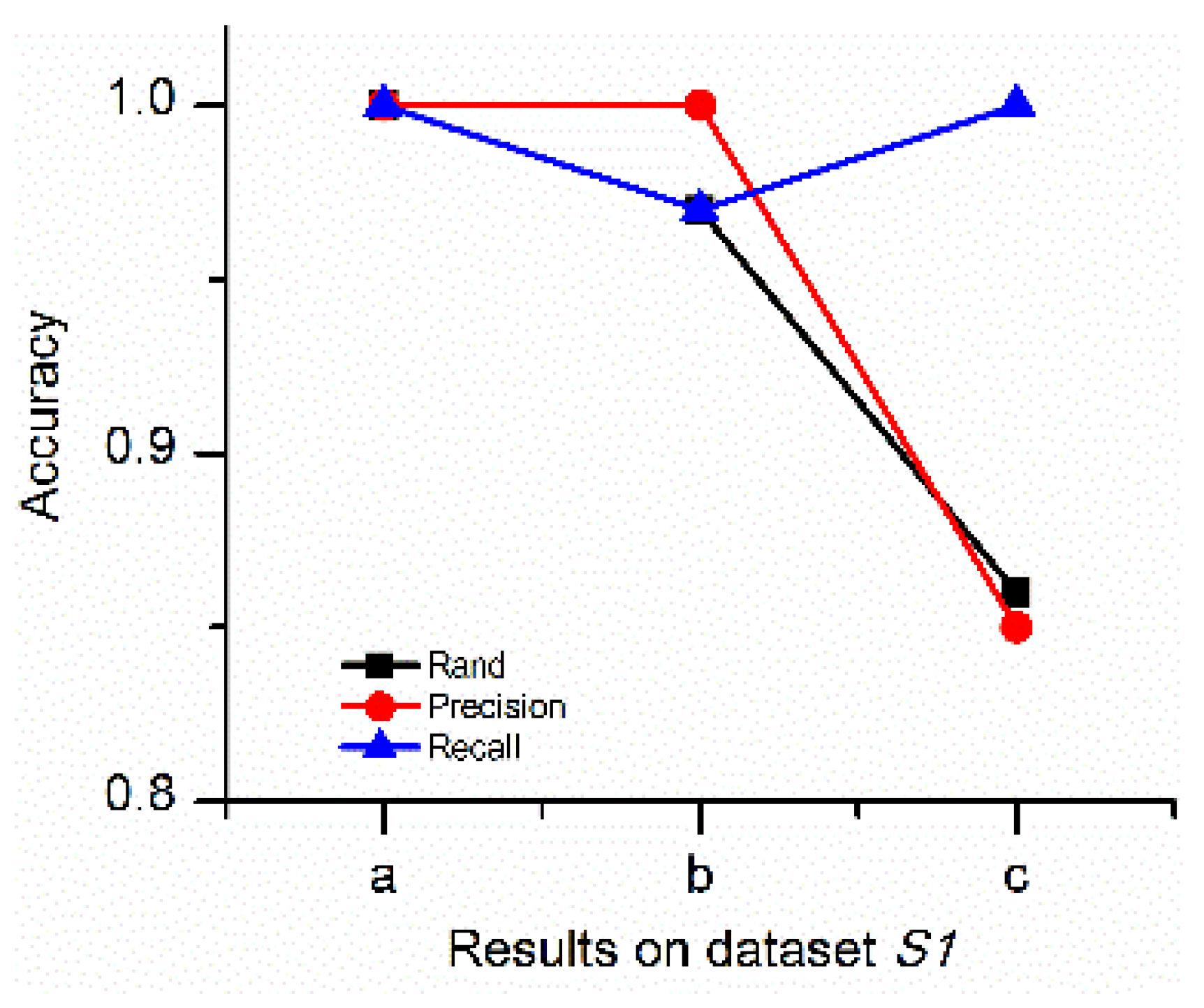
3.3. Accuracy Evaluation of Clustering Results

The literature provides several indexes that are useful for evaluating clustering results [17,18]. These indexes can evaluate the results of different clustering algorithms for the same dataset. The detailed calculation methods are discussed as follows.

The Rand index assesses the ability of a particular cluster detection approach to find the known clusters and noises. The index is expressed as follows:

$$Rand=\raisebox{1ex}{$T_P+T_N$}\!\left/ \!\raisebox{-1ex}{$T_P+F_P+F_N+T_N$}\right.$$

(7)

where $T_P$ is a true positive decision (i.e., the count of the points in correctly detected clusters based on the mapping functions [19]), $F_P$ is a false positive decision (i.e., the count of the points in incorrectly detected clusters), $T_N$ is a true positive decision (i.e., the total number of the correctly detected noises), and $F_N$ is a false negative decision (i.e., the total number of incorrectly detected noises). An issue of the accuracy index involves the simultaneous consideration of false positives and false negatives. To address this issue, another two indexes, precision and recall are further applied to assess the accuracy [18].

Recall evaluates the ability of the clustering algorithm to identify the positive detection success and is defined as follows:

$$Recall=\raisebox{1ex}{$T_P$}\!\left/ \!\raisebox{-1ex}{$T_P+F_N$}\right.$$

(8)

Precision captures the subtleties of the clustering algorithm and is defined as follows:

$$Precision=\raisebox{1ex}{$T_P$}\!\left/ \!\raisebox{-1ex}{$T_P+F_P$}\right.$$

(9)

Notably, the accuracy of the results is judged by all three indexes. For two clustering results $r1$ and $r2$ of the same dataset, the final evaluating results are denoted as $\left\{Rand\left(r1\right),recall\left(r1\right),precision\left(r1\right)\right\}$ and $\left\{Rand\left(r2\right),recall\left(r2\right),precision\left(r2\right)\right\}$, respectively. $r1$ is regarded as the better result if its indexes meet one of the following criteria.

Criterion 1: 

$recall\left(r1\right)>recall\left(r2\right)$ and $precision\left(r1\right)>precision\left(r2\right)$.

Criterion 2: 

$recall\left(r1\right)>recall\left(r2\right)$, $precision\left(r1\right)<precision\left(r2\right)$ and $Rand\left(r1\right)>Rand\left(r2\right)$.

4. Results

Simulated datasets and real applications are designed and utilized to verify the effectiveness and accuracy of DTSC. Simulated datasets are set according to several earlier studies about simulated dataset designation [20] and characteristics of real applications. A detailed validation of the DTSC algorithm on simulated datasets is given in Section 4.1. Rainfall data in Mainland China from 1960 to 2009 are investigated using the proposed DTSC to mine the distribution characteristics of rainfall to validate the advantages of DTSC further. The case study of Rainfall data using DTSC is thoroughly described in Section 4.2.

4.1. Validation of DTSC Algorithm on Simulated Datasets

This Section conducts three experiments based on simulated datasets to validate the effectiveness and accuracy of the DTSC algorithm. Simulated datasets are designed to verify the feasibility and accuracy of DTSC, as shown in Section 4.1.1. In Section 4.1.2, the efficiency of the proposed DTSC algorithm is then illustrated by comparing the DTSC with a typical algorithm (the density-based time series clustering algorithm) [6]. Experiment 2 in Section 4.1.3 is conducted to evaluate the effectiveness of the proposed parameter optimization method that was proposed in Section 3.1. Results with an optimal parameter and non-optimal parameters are compared with each other using the above-mentioned accuracy evaluation functions (see Section 3.3). Experiment 3 in Section 4.1.4 is utilized to validate the feasibility of the proposed similarity measurements that have been described in Section 2.1, which is achieved by comparing clustering results based on the proposed similarity measurements with those obtained based on typical similarity measurements.

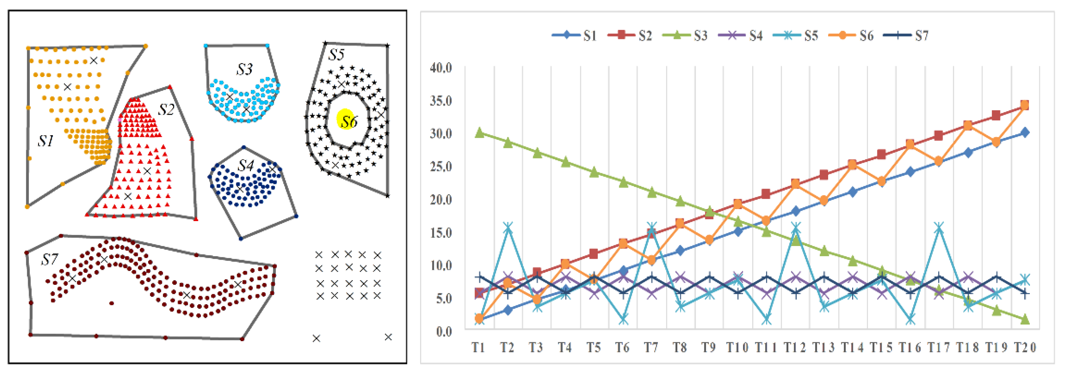
4.1.1. Validation of DTSC Algorithm Based on Simulated Dataset

To provide a reasonable simulated dataset for evaluating the performance of the DTSC algorithm, simulated datasets $S1$ (see Figure 4 and Figure 5) and $S2$ (see Figure 6 and Figure 7) are designed based on the characteristics of real applications and by referring to earlier studies [20].

The characteristics of $S1$ and $S2$ are described below.

(1)

$S1$ and $S2$ contain 759 and 806 objects, respectively,

(2)

The time dimensionality is 20 and the neighboring time intervals are equal,

(3)

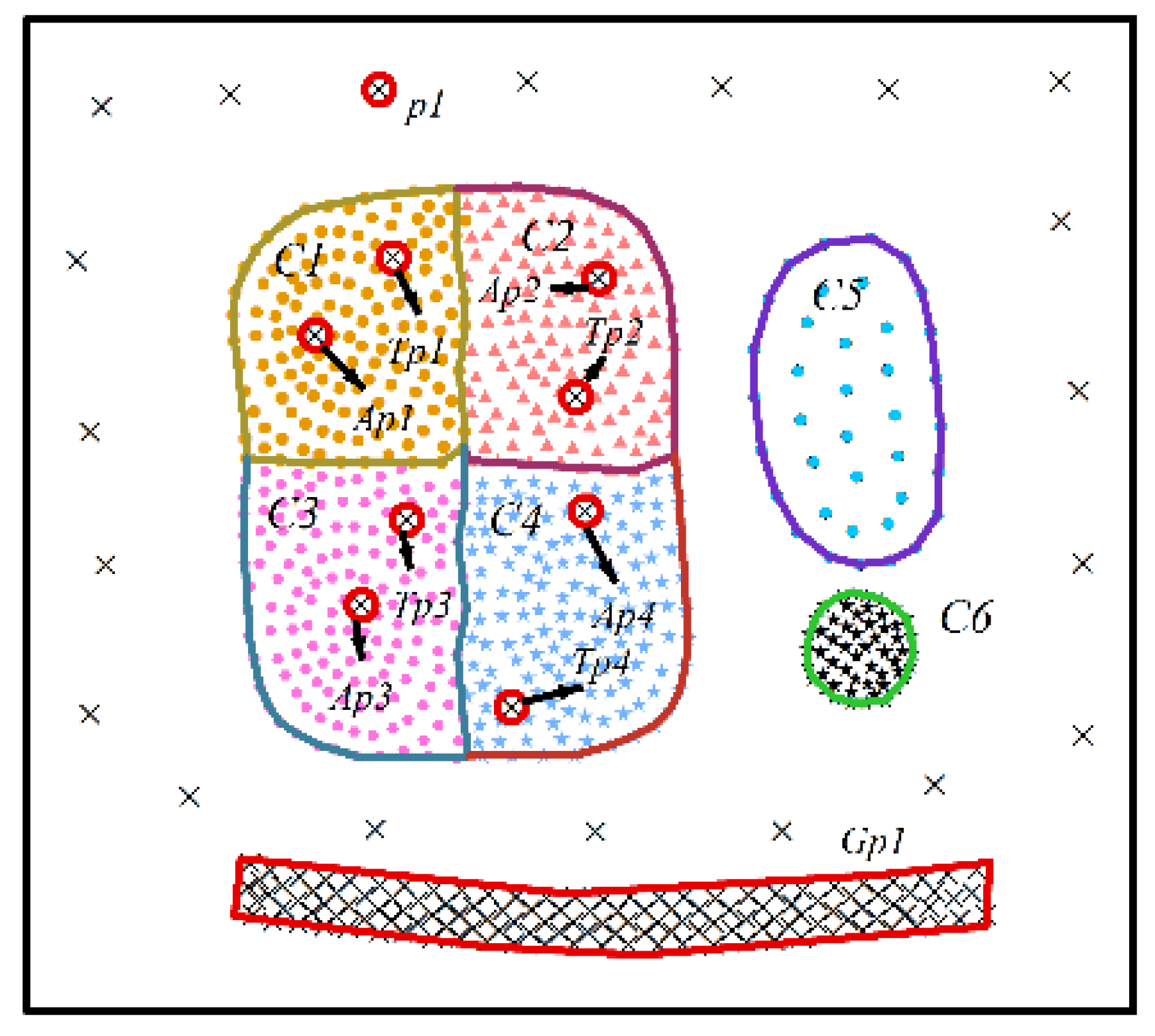
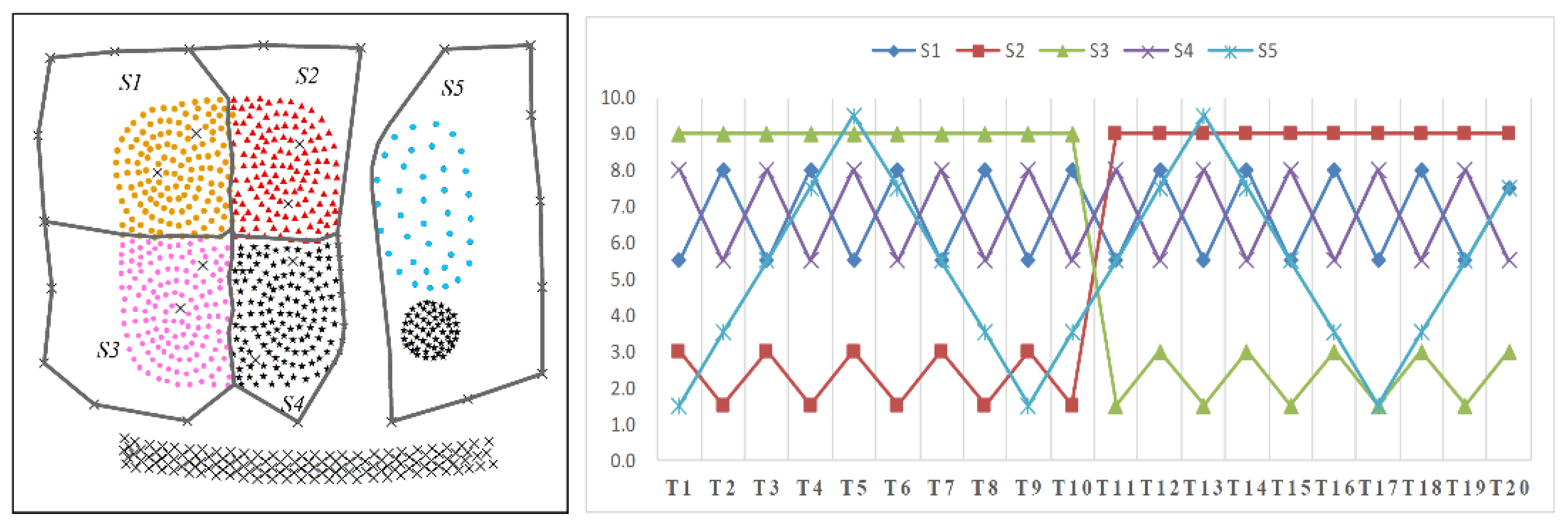
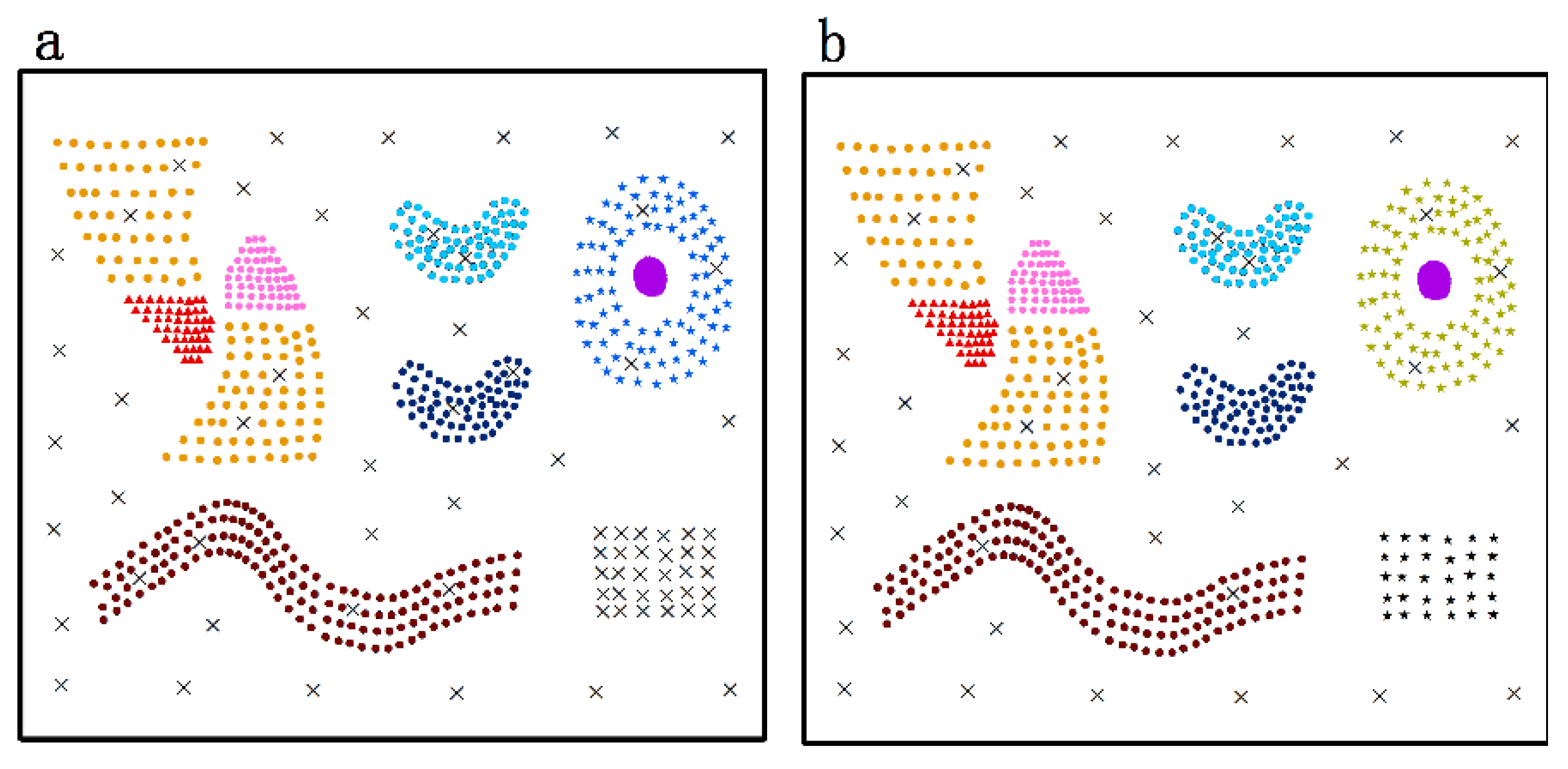
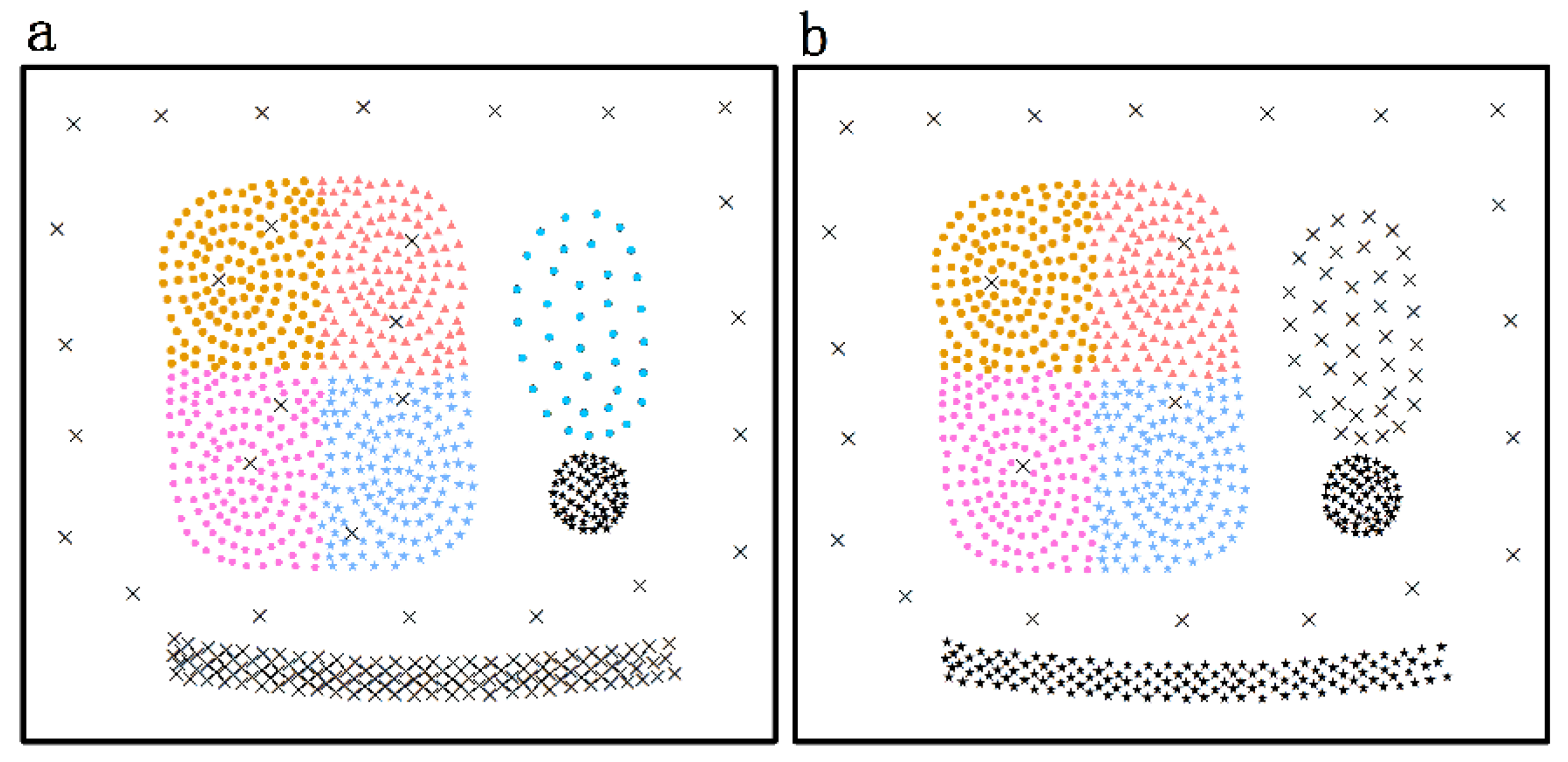
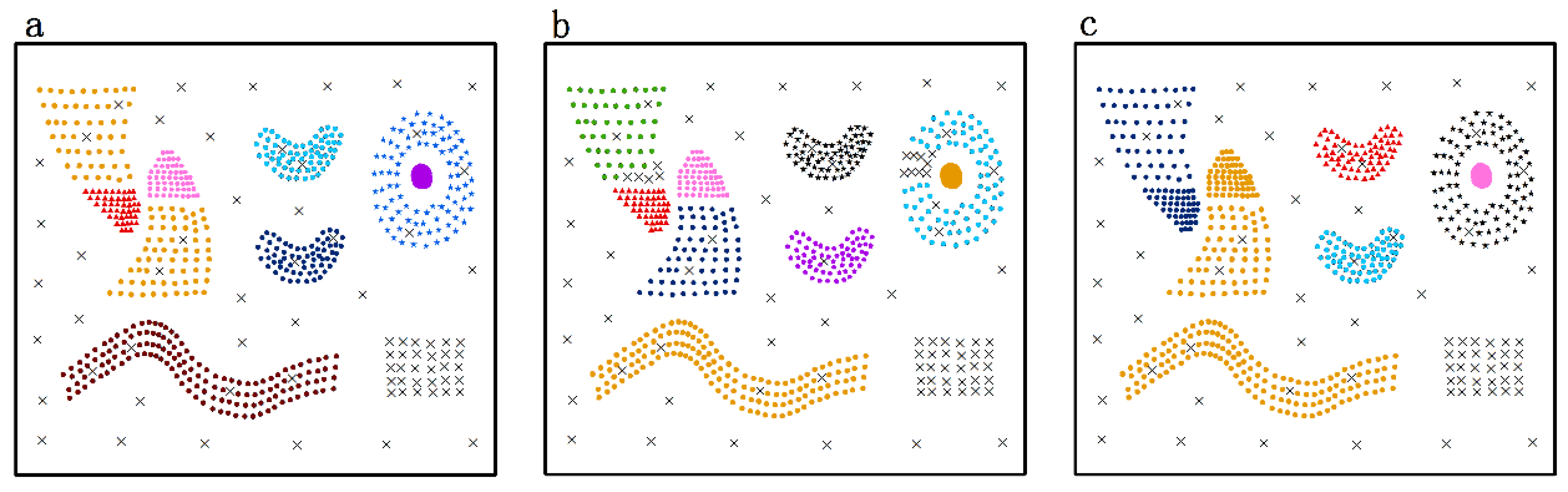
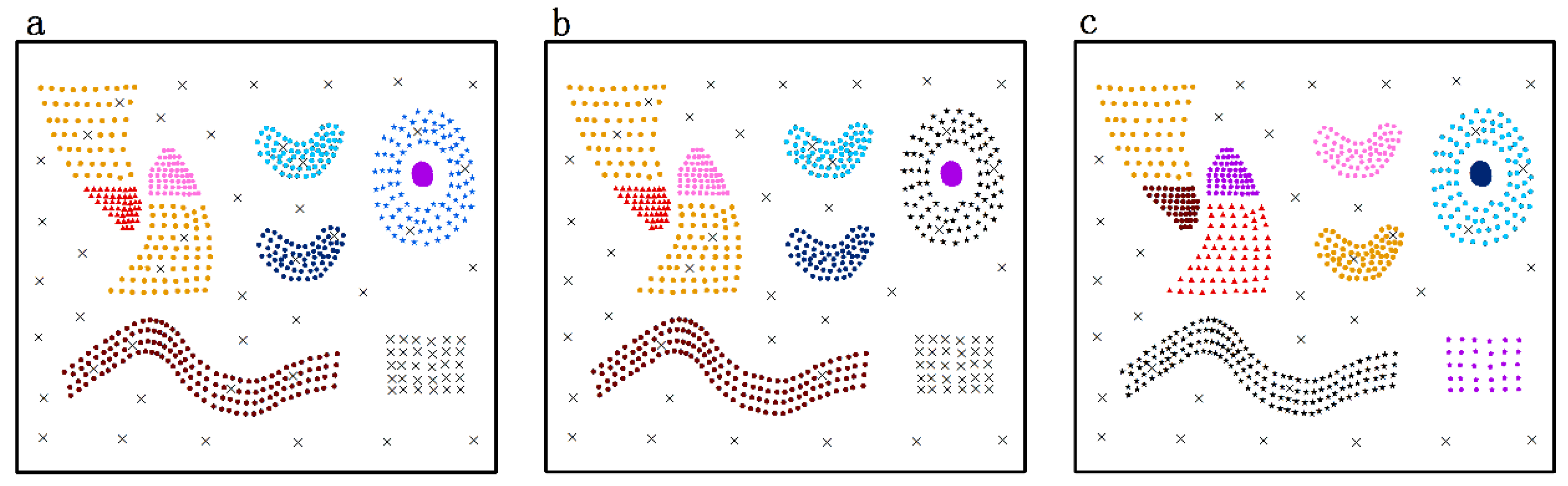
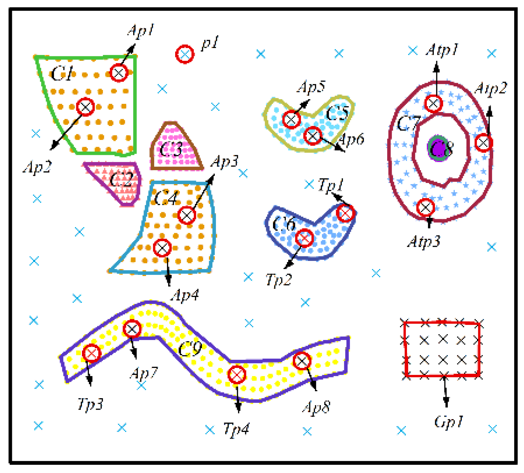
Nine predefined clusters labeled as $C1$ to $C9$ in $S1$ (in Figure 4) and five predefined clusters labeled as $C1$ to $C5$ in $S2$ (in Figure 6) exist. These clusters possess arbitrary geometrical shapes and different densities. The non-spatial attributes of the cluster at every time point are randomly distributed under one range, and the mean value of attributes in every cluster are shown in Figure 5 and Figure 7,

(4)

To maintain consistency with the real applications, noises are set in the simulated datasets and are classified into five types. Type 1 comprises the spatial noises that have a meaning similar to that of spatial outliers whose spatial attribute values are significantly different from those of other objects in their spatial neighborhood; these are labeled as $p$ (such as $p1$). The non-spatial attributes of spatial noises are similar to the nearest clusters in dataset $S1$. Types 2 and 3 are the non-spatial attribute noises and non-spatial attribute trend noises, respectively, which are labeled as $Ap$ (such as$Ap1$ to $p8$) and $Tp$ (such as $Tp1$ to $Tp4$), respectively. The attributes of these types of noises are significantly different from those of their neighboring objects. Type 4 comprises noises whose attribute values and attribute trends are both significantly different from those of neighboring objects; these noises are labeled as $Atp$ (such as $Atp1$ to $Atp3$). Type 5 comprises gradually changing noises, whose attribute values change in a descending or ascending fashion along the spatial position although their attribute trends are similar. For example, the temperature decreases as the altitude increases, and the temperature trend is similar at different altitudes with seasonal variations. These gradually changing noises are labeled as $Gp$ (such as $Gp1$).

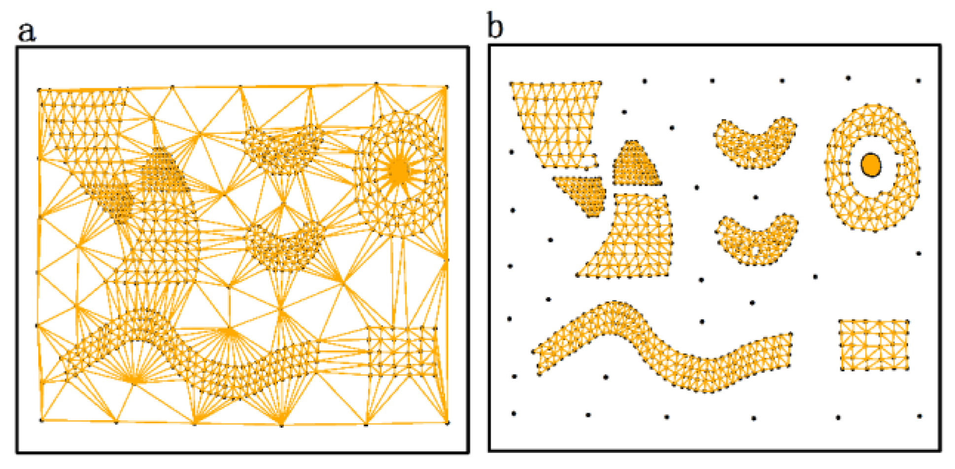
4.1.2. Comparison between DTSC and Typical Algorithms

Experiments are conducted on simulated datasets to verify the efficient and accuracy of DTSC algorithm in comparison with the density-based time series clustering algorithm, which also considers spatial and non-spatial attributes. Density-based time series clustering algorithm is based on the Euclidean distance-based similarity measurement method. Parameters in the density-based time series clustering algorithm are complex and comprise spatial radii and the threshold of attributes. In the density-based time series algorithm, when objects in the radius of an object p whose attribute distances from p are less than the threshold of attributes are iteratively aggregated. Optimal values of these parameters are difficult to obtain; hence, we conduct a parametric study to obtain the most appropriate result. The parametric study runs the proposed programs approximately 20 times.

The results of DTSC algorithm on $S1$ and $S2$ are obtained according to the steps in Section 3 as follows: First, the spatial proximity relationships based on the Delaunay triangulation are obtained by using the strategy in Section 3.1 and are shown in Figure 8 and Figure 9. Second, the clusters with similar spatial and non-spatial attributes (in Figure 10a and Figure 11a) are detected by adopting the proposed method in Section 3.2. Finally, the accuracy evaluation values of the results are shown in

Table 1. Accuracy values of clustering results on simulated datasets and its corresponding computation cost time.

Clustering Results	Simulated Dataset		Accuracy Values			Computation Cost
	$\mathit{S}1$	$\mathit{S}2$	Rand	Precision	Recall	Time (s)
Results of DTSC	√		1	1	1	5
Results of density-based time series clustering algorithm	√		0.95	0.95	1	4
Results of DTSC		√	1	1	1	4
Results of density-based time series clustering algorithm		√	0.65	0.55	0.44	3

.

For comparison, the clustering results of the density-based time series clustering algorithm are shown in Figure 10b and Figure 11b. A cluster is labeled as the same symbol with the same color, and noises are labeled with a black “x”. The figures show that the density-based time series clustering algorithm is sensitive to noises. For example, noises $Tp1$ to $Tp4$ (in $S1$ and $S2$) are incorrectly recognized as a part of the neighboring clusters and the gradually changing noises $Gp1$ (in $S1$ and $S2$) are incorrectly detected as a cluster. In addition, density-based time series clustering algorithm is unsuitable for clusters with different densities. $C4$ (in $S2$), with a relatively low density, is incorrectly recognized as noises. The computation cost of the methods in Table 1 show that both methods are highly efficient. Combing the accuracy evaluation indexes, we can see that the proposed DTSC algorithm can efficiently and accurately detect non-overlapping clusters with arbitrary shapes and uneven distributions of spatial and non-spatial time series attributes.

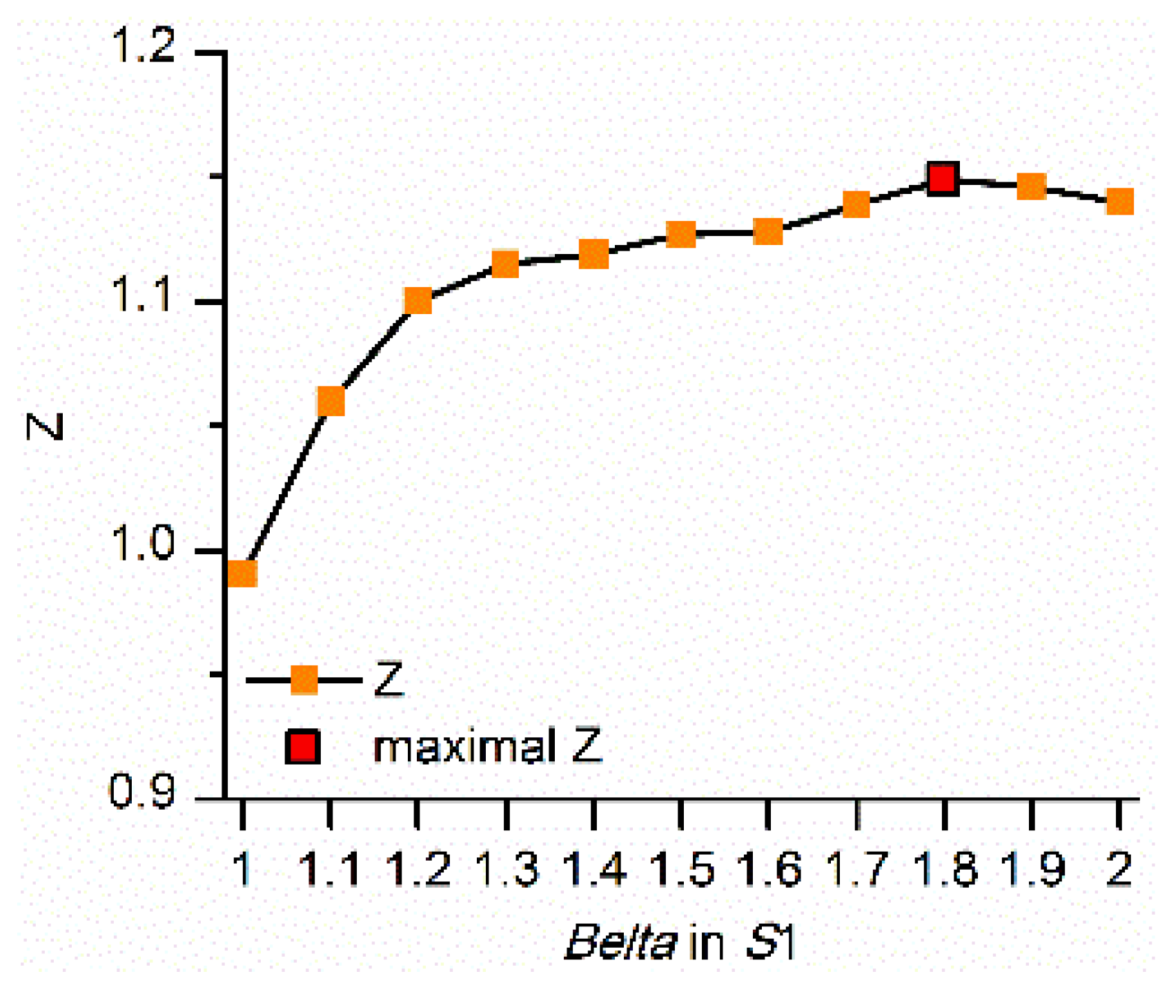
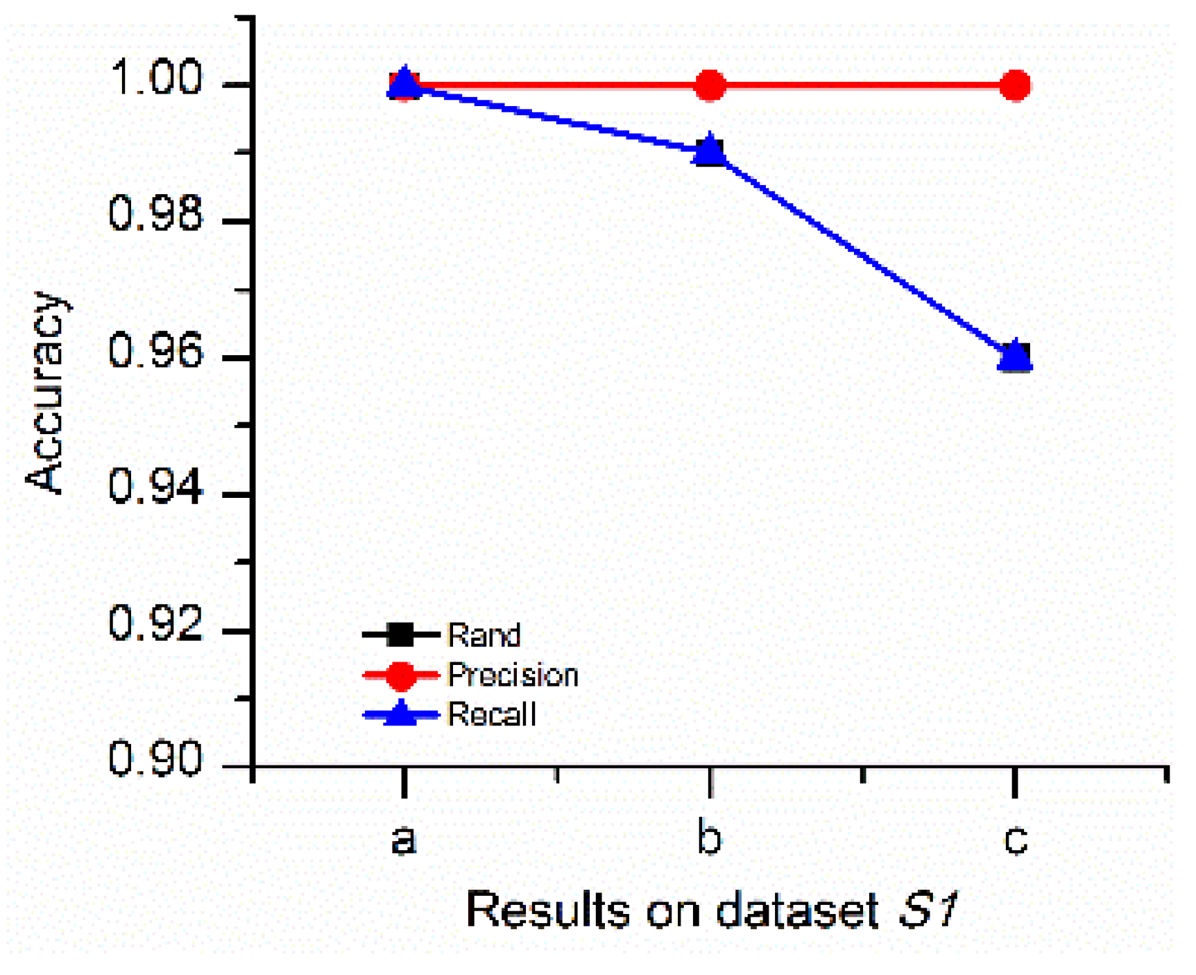
4.1.3. Comparison of the DTSC Algorithm with Optimal and Non-Optimal Parameters in the Spatial Domain

This Section evaluates the applicability of the parameter optimizing method described in Section 3.1. Clustering results of $S1$ obtained by the DTSC algorithm with optimal and non-optimal parameters are compared. The optimal value of parameter $\beta$ (In Equation (4)) with the largest parameter evaluation function $\mathrm{Z}$ (in Figure 12) is automatically obtained by utilizing the parameter optimizing method. The non-optimal parameter $\beta$, which is significantly different with each other and the optimal parameter, is set among the ranges of the parameter.

Clustering results on $S1$ (in Figure 13) show that the value of the parameter strongly affects the result. When the parameter is small, several clusters, such as $C1$ and $C7$, are over-segmented, and several objects in these clusters are incorrectly recognized as noises. When the parameter is large, the neighboring clusters with different density are recognized as the same cluster. For example, neighboring clusters $C1$ and $C2$ with different densities are recognized as the same cluster. Through the accuracy evaluation values in Figure 14, we can see that the result with the optimal parameter can detect clusters and noises with the highest accuracy relative to the results of non-optimal parameters.

4.1.4. Comparison of the DTSC Algorithm with Proposed Similarity Measurements and Typical Similarity Measurements in the Non-Spatial Domain

As illustrated in Section 2.1, the similarity measurement method is a key component of the clustering algorithm. Experiments are conducted based on the proposed similarity measurements, Euclidean distance similarity measurement and Pearson correlation coefficient similarity measurement to verify the proposed similarity measurements. Results on $S1$ are shown in Figure 15. Result of DTSC based on Euclidean distance (Figure 15b) shows that noises of type 3 are unable to be detected. For example, noises $Tp1$ to $Tp4$ (Figure 15b) with significantly different attribute trends from their neighbors are incorrectly recognized as a part of the neighboring cluster. Result of DTSC based on Pearson correlation coefficient (Figure 15b) indicates that attribute noises of types 2 and 4 cannot be correctly recognized by this method. For example, noises $Ap1$ to $Ap8$ (Figure 15c) are incorrectly recognized as a part of the neighboring clusters and gradually changing noises $Gp1$ (Figure 15c) are also incorrectly detected as a cluster. Both the result of DTSC based on the proposed similarity measurements (Figure 15a) and the accuracy result (Figure 16) indicate that the accuracy of DTSC with the proposed similarity measurements is highest; therefore, the proposed similarity measurements are effective.

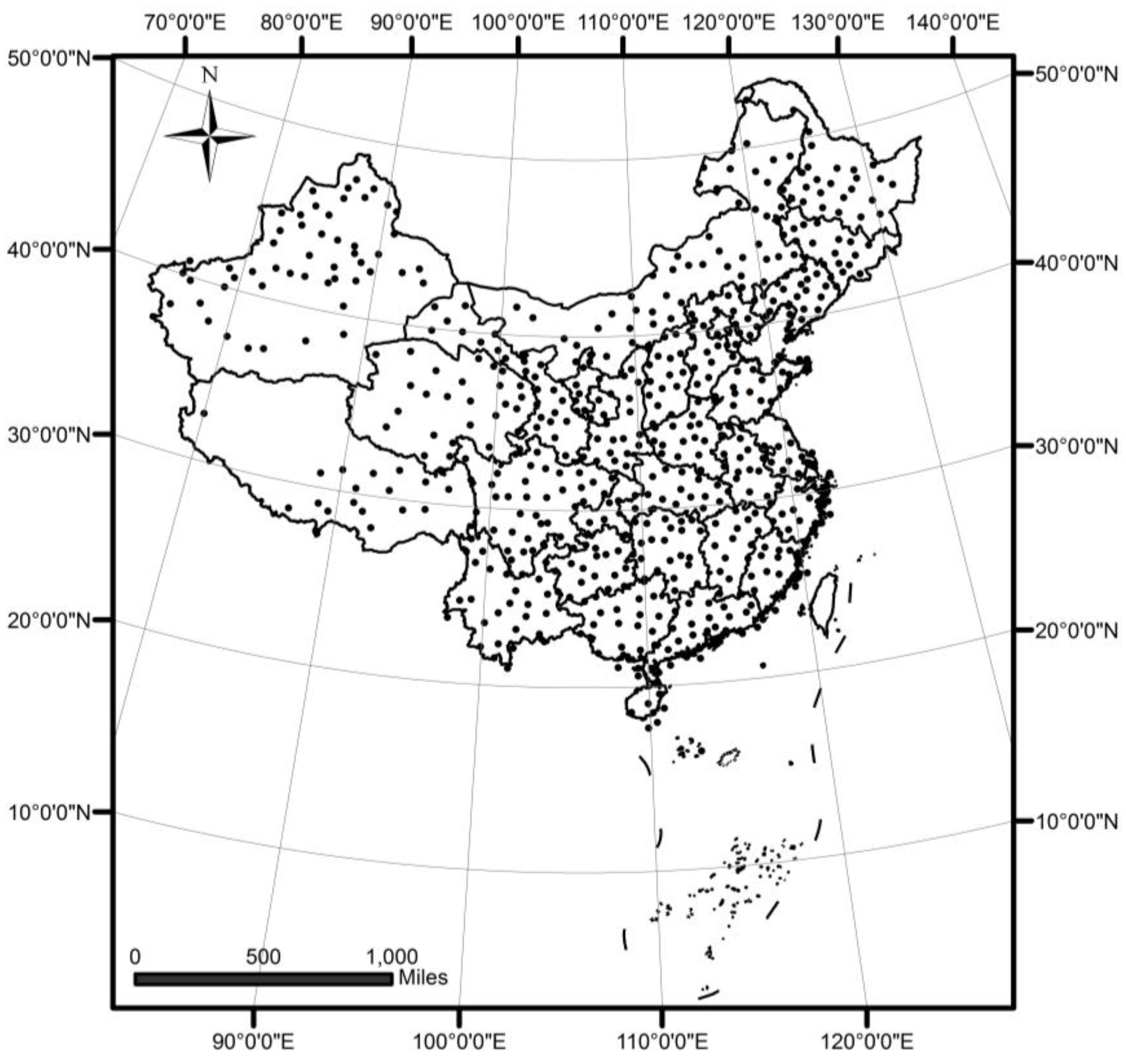
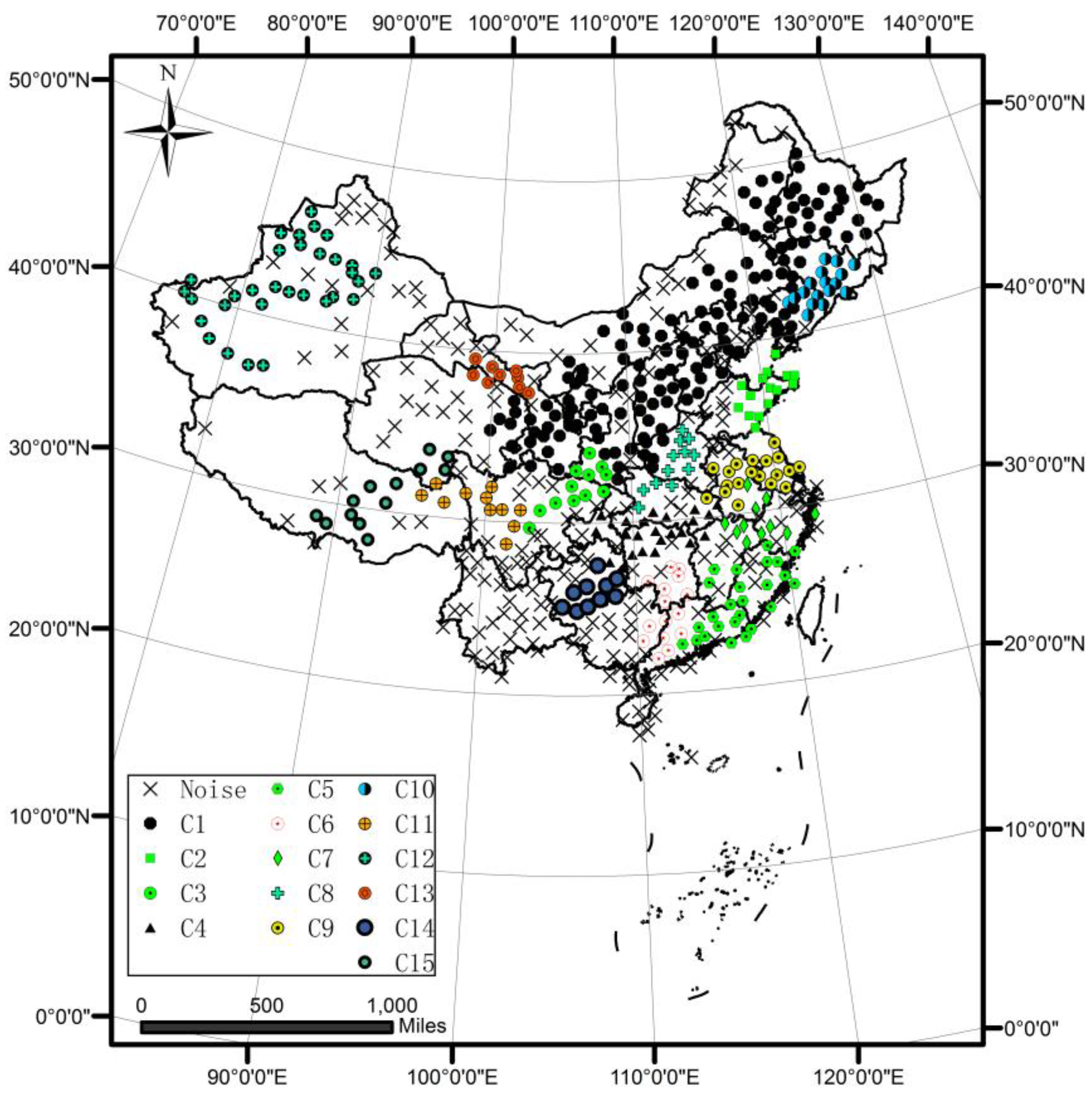
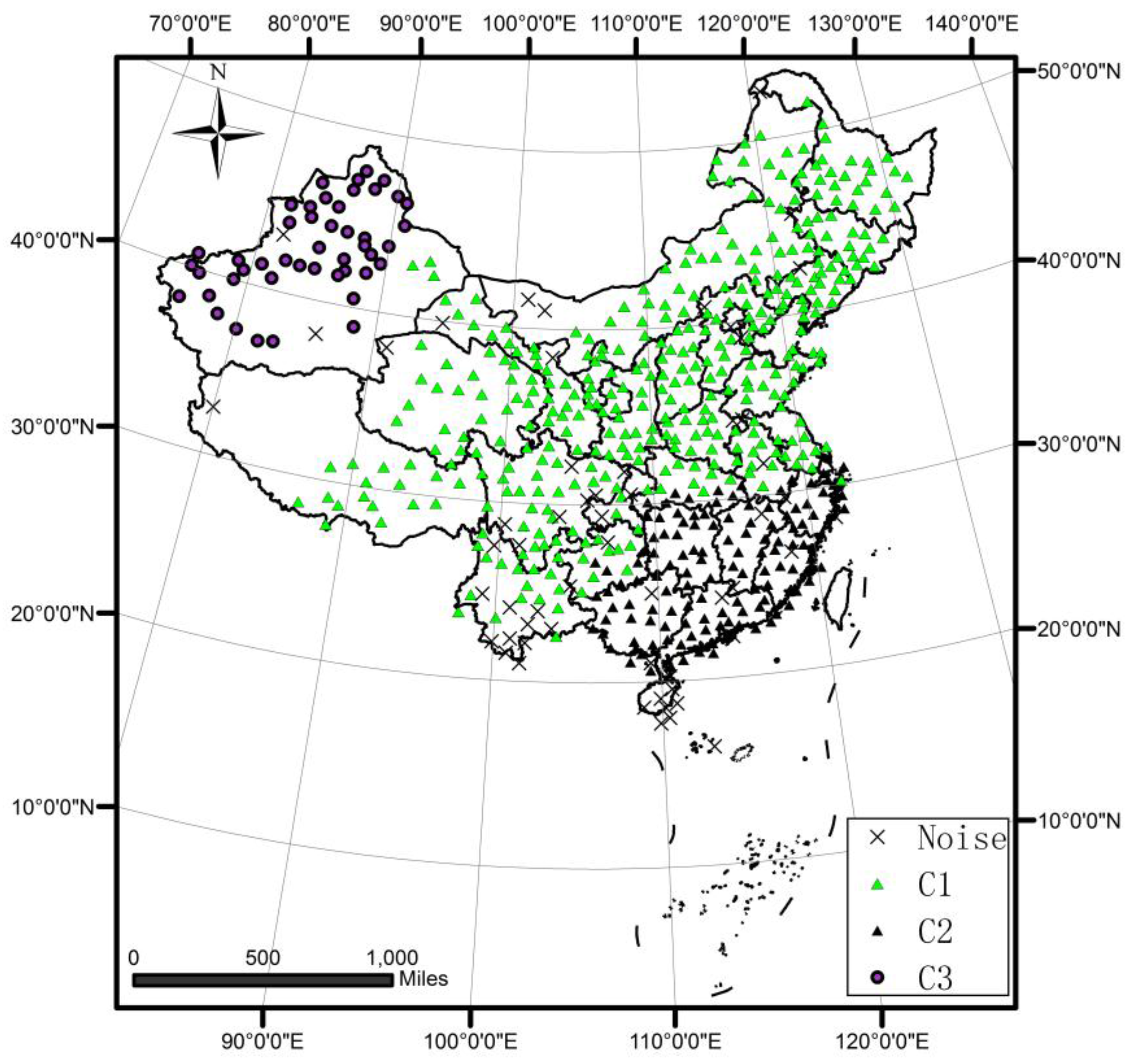
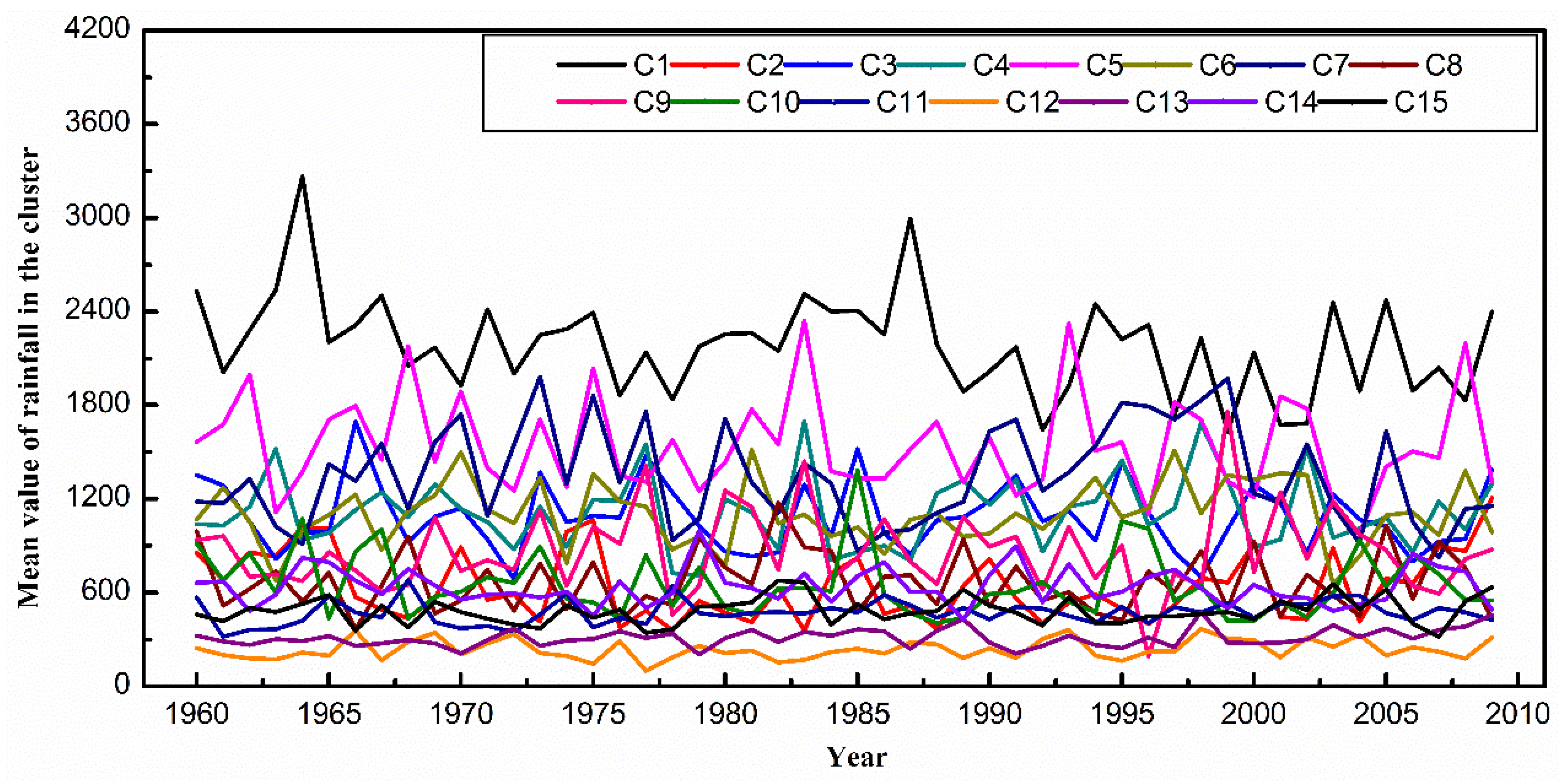
4.2. A Case Study of DTSC on Rainfall Data

The distribution of rainfall is significantly affected by the geographic location, topography, temperature and the distance to oceans, lakes and other factors, which thus suggests that the distribution of rainfall generally exists strong spatial heterogeneity. Characteristics of the clustering distribution of the rainfall provide the basis for further mining of the rainfall mechanism. This clustering will improve future rainfall prediction efforts. Time series clustering methods can accurately detect clustering distribution features of phenomena without compromising generality. The proposed DTSC algorithm is thus applied to the annual rainfall data to mine the clustering pattern of rainfall. These data are provided by the China Meteorological Bureau and comprise the annual average rainfall monitoring data of 599 rainfall stations in Mainland China from 1960 to 2009. The locations of rainfall stations are shown in Figure 17.

The distribution trend of the rainfall in China during the studied period decreases progressively from the southeast to the northwest. The clustering result is shown in Figure 18 and Figure 19. Several interesting patterns, which will be described in detail in the following paragraph, are discovered in the results. For comparison, the density-based time series clustering algorithm is also utilized in the dataset, and its result is shown in Figure 20.

Figure 18 shows that 15 interesting clusters were obtained. The mean and standard deviation of the clusters at every time point are listed in Figure 19 and

Table 2. Statistics of clusters in Figure 18 and Figure 20.

Statistical Variables	Statistics of the Clusters
	C1	C2	C3	C4	C5	C6	C7	C8	C9	C10	C11	C12	C13	C14	C15
Value (Figure 18)	171	153	168	150	189	160	136	169	148	167	50	98	146	162	106
Value (Figure 20)	373	310	180

. The neighboring clusters are significantly different in terms of non-spatial time series attribute values and trends. The distribution and statistics of clusters show that rainfall gradually increased from the northwestern to southeastern areas. Clusters C1, C12, C13 and C15 in the northern and eastern areas have low rainfall and are relatively stable. However, the other clusters in the eastern and southern parts experience abundant rainfall and fluctuate heavily over time. In these areas, clusters with significantly different time series attribute values and trends or that are separated by noises are correctly recognized by the proposed DTSC algorithm. Furthermore, Hou et al. [21] stated that separating line between C1 and C2, C3, C8 and C10 is consistent with the line of semi-humid and semi-arid regions; these results are consistent with actual conditions. Regions recognized as noises are unstable and vary highly in the spatial domain; these regions can serve as the basis for outlier events and extreme climate phenomena.

Compared with the result of the density-based time series clustering algorithm in Figure 20, clusters with significantly different time series attribute values and trends are recognized as the same clusters. Combing the statistics in Table 2, we can see that the standard deviations of clusters are seriously larger than the result obtained by the DTSC algorithm.

In summary, two important findings are obtained from the application of the DTSC to the rainfall data. First, clusters with similar time series attribute values and trends are detected using DTSC algorithm. Second, the characteristics of clusters are analyzed by combining their statistics and existing studies; this combination provides an important reference for rainfall mechanism analysis and forecasting.

5. Discussion and Further Work

In this paper, a DTSC algorithm was proposed to adaptively detect the clusters of objects with spatial proximity and similar time series attribute values and trends. The proposed algorithm uses two important techniques to realize an automatic procedure for detecting clusters. The first technique is the combinational use of the operation of constructing spatial proximity in DBSC and PSO, which contributes significantly to realizing the automatic discovering of spatially homogenous object sets with spatial proximity, similar densities and arbitrary shapes. The other technique is to combine the strategy of non-spatial clustering in DBSC with the proposed similarity measurements, based on which the DTSC can correctly recognize the non-overlapping clusters with similar time series attribute values and trends.

The experiments on the simulated datasets and a real application have validated the efficiency of the DTSC algorithm. Several conclusions are therefore summarized as follows. First, the DTSC algorithm can separate objects with different densities and prevent over-segmentation and under-segmentation by using PSO. Second, the DTSC algorithm automatically detects clusters with similar spatial attributes and non-spatial time series attribute values and trends. Third, compared with the traditional algorithms that detect clusters but require several predefined parameters, the DTSC algorithm can adaptively mine the distribution features of data without sufficient prior knowledge. Fourth, noises with significantly different attributes from neighbors can be recognized easily with a reasonable accuracy. Lastly, the DTSC algorithm is more efficient and precise than the typical algorithms when addressing clusters with arbitrary shapes, different densities and unevenly distributed attributes under the interference of spatial and non-spatial noises.

Based on the current study, future studies should focus on: (1) enhancing the computing efficiency of DTSC using more advanced strategies such as the dimensionality reduction method [22]; (2) extending the DTSC to applications with multiple variables; and (3) combining the association rules with the DTSC to mine the association of clusters with other coexisting factors which can provide basic information for further mechanism analysis.

References

- Guyet, T.; Nicolas, H. Long term analysis of time series of satellite images. Pattern Recognit. Lett. 2016, 70, 17–23. [Google Scholar] [CrossRef]
- Bidari, P.S.; Manshaei, R.; Lohrasebi, T.; Feizi, A.; Malboobi, M.A.; Alirezaie, J. Time series gene expression data clustering and pattern extraction in arabidopsis thaliana phosphatase-encoding genes. In Proceedings of the 8th IEEE International Conference on BioInformatics and BioEngineering, Athens, Greece, 8–10 October 2008; pp. 1–6.
- Kaur, G.; Dhar, J.; Guha, R.K. Minimal variability owa operator combining anfis and fuzzy c-means for forecasting bse index. Math. Comput. Simul. 2016, 122, 69–80. [Google Scholar] [CrossRef]
- Yin, J.; Zhou, D.; Xie, Q.Q. A clustering algorithm for time series data. In Proceedings of the 7th International Conference on Parallel and Distributed Computing, Applications and Technologies, Taipei, Taiwan, 4–7 December 2006; pp. 119–122.
- Uijlings, J.R.R.; Duta, I.C.; Rostamzadeh, N.; Sebe, N. Realtime video classification using dense HOF/HOG. In Proceedings of the ICMR 2014: International Conference on Multimedia Retrieval, Glasgow, UK, 1–4 April 2014; pp. 145–152.
- Chandrakala, S.; Sekhar, C.C. A density based method for multivariate time series clustering in kernel feature space. In Proceedings of the 2008 IEEE International Joint Conference on Neural Networks (IEEE World Congress on Computational Intelligence), Hongkong, China, 1–8 June 2008.
- Yeang, C.; Jaakkola, T. Time series analysis of gene expression and location data. Int. J. Artif. Intell. Tools 2003, 14, 305–312. [Google Scholar] [CrossRef]
- Xu, T.; Shang, X.; Yang, M.; Wang, M. Bicluster algorithm on discrete time-series gene expression data. Appl. Res. Comput. 2013, 30, 3552–3557. [Google Scholar]
- Yan, L.; Kong, Z.; Wu, Y.; Zhang, B. Biclustering nonl inearly correlated time series gene expression data. J. Comput. Res. Dev. 2008, 45, 1865–1873. [Google Scholar]
- Liu, Q.; Deng, M.; Shi, Y.; Wang, J. A density-based spatial clustering algorithm considering both spatial proximity and attribute similarity. Comput. Geosci. 2012, 46, 296–309. [Google Scholar] [CrossRef]
- Ramirez-Lopez, L.; Schmidt, K.; Behrens, T.; van Wesemael, B.; Demattê, J.A.M.; Scholten, T. Sampling optimal calibration sets in soil infrared spectroscopy. Geoderma 2014, 226–227, 140–150. [Google Scholar] [CrossRef]
- Chan, C.-W. Modified particle swarm optimization algorithm for multi-objective optimization design of hybrid journal bearings. J. Tribol. 2014, 137. [Google Scholar] [CrossRef]
- Liu, Q.; Deng, M.; Shi, Y. Adaptive spatial clustering in the presence of obstacles and facilitators. Comput. Geosci. 2013, 56, 104–118. [Google Scholar] [CrossRef]
- Liu, Y.; Wang, X.; Liu, D.; Liu, L. An adaptive dual clustering algorithm based on hierarchical structure: A case study of settlements zoning. Trans. GIS 2016, in press. [Google Scholar]
- Liu, Q.; Deng, M.; Peng, D.; Wang, J. Validity assessment of spatial clustering methods based on gravitational theory. Geomat. Inf. Sci. Wuhan Univ. 2011, 36, 982–986. [Google Scholar]
- Guo, W.Z.; Chen, J.Y.; Chen, G.L.; Zheng, H.F. Trust dynamic task allocation algorithm with nash equilibrium for heterogeneous wireless sensor network. Secur. Commun. Netw. 2015, 8, 1865–1877. [Google Scholar] [CrossRef]
- Grubesic, T.H.; Wei, R.; Murray, A.T. Spatial clustering overview and comparison: Accuracy, sensitivity, and computational expense. Ann. Assoc. Am. Geogr. 2014, 104, 1134–1156. [Google Scholar] [CrossRef]
- Sanderson, M.; Christopher, D. Manning, Prabhakar Raghavan, Hinrich Schütze, Introduction to Information Retrieval; Cambridge University Press: Cambridge, UK, 2008. [Google Scholar]
- Meng, F.; Li, X.; Pei, J. A feature point matching based on spatial order constraints bilateral-neighbor vote. IEEE Trans. Image Process. 2015, 24, 4160–4171. [Google Scholar] [CrossRef] [PubMed]
- Nosovskiy, G.V.; Liu, D.; Sourina, O. Automatic clustering and boundary detection algorithm based on adaptive influence function. Pattern Recognit. 2008, 41, 2757–2776. [Google Scholar] [CrossRef]
- Hou, G.; Wang, J.; Guo, Q.; Yan, X. A study on the cumulative distributions of rainfall rate R_1 (0.01) over China. J. Beijing Inst. Technol. 2002, 22, 262–264. [Google Scholar]
- Keogh, E.; Chakrabarti, K.; Pazzani, M.; Mehrotra, S. Dimensionality reduction for fast similarity search in large time series databases. Knowl. Inf. Syst. 2002, 3, 263–286. [Google Scholar] [CrossRef]