Processing: A Python Framework for the Seamless Integration of Geoprocessing Tools in QGIS

Abstract

Processing is an object-oriented Python framework for the popular open source Geographic Information System QGIS, which provides a seamless integration of geoprocessing tools from a variety of different software libraries. In this paper, we present the development history, software architecture and features of the Processing framework, which make it a versatile tool for the development of geoprocessing algorithms and workflows, as well as an efficient integration platform for algorithms from different sources. Using real-world application examples, we furthermore illustrate how the Processing architecture enables typical geoprocessing use cases in research and development, such as automating and documenting workflows, combining algorithms from different software libraries, as well as developing and integrating custom algorithms. Finally, we discuss how Processing can facilitate reproducible research and provide an outlook towards future development goals.

1. Introduction

Geographic information systems (GIS) have found widespread adoption in public administration, industry and a multitude of research disciplines thanks to their capabilities to integrate heterogeneous digital data and to provide data analysis, as well as their visualization functionality [1,2]. The development of GIS follows two principal development paradigms [3,4]: the open source or the closed source (often proprietary) development model. In the open source model, the source code is typically published under a free software license, which grants the user four essential freedoms [5,6]: the rights to run the code for any purpose, to study how the code works and to modify it, to redistribute copies and even to redistribute modified copies.

QGIS [7] (formerly known as Quantum GIS) is one of the most popular open source GIS with a growing user base and increasing importance in the education sector (see, for example, the courses offered by [8,9]). It is a multi-purpose open source GIS, which can be used for spatial data creation, editing, analysis and mapping. Besides the desktop GIS application, the QGIS project also provides server and related web mapping applications, as well as versions adapted to the requirements of mobile devices.

Processing is an object-oriented Python framework for QGIS. Although QGIS did include geoprocessing tools before Processing was introduced, it lacked a comprehensive framework for spatial analysis. The main goal of Processing is to provide a platform for the development of analysis algorithms that makes it easy to implement and use these algorithms.

The remainder of this paper is structured as follows: Section 2 provides background information about the development history of the QGIS Processing framework and similar existing technology. Section 3 describes the software architecture, algorithm integration for different source libraries, as well as the current limitations of the framework. Section 4 presents a review of selected applications, and Section 5 summarizes the key points and discusses room for further development.

2. Background

QGIS is an open source GIS project, which was started in 2002. The initial goal of the QGIS project was to create a spatial data viewer [7]. Today, QGIS has reached a point in its evolution where it is used by a wide variety of users for daily spatial data viewing, editing, and analysis tasks [10], as well as in education (for example, [8,9]). QGIS runs on most Linux and Unix platforms, Windows and Mac OS X and has been published under the GNU (a collection of free software; the acronym stands for “GNU’s not Unix”) General Public License (GPL). The QGIS core is developed using the Qt toolkit and C++. Additionally, QGIS provides a Python application program interface (API), which is used to expand its functionality. As [11] note, a “powerful Python interface can help to efficiently exploit the capabilities of a GIS” and integrate different tools and programming languages to expand it. This effect, an increasing number of contributions, has been very noticeable since the introduction of the QGIS Python API in QGIS 0.9 in 2007 when new developers started to add functionality using Python plugins.

2.1. Processing Goals and Motivation

The main goal of Processing is to create a platform for the development of geoprocessing algorithms that makes it easy to implement and use these algorithms. Although QGIS did include geoprocessing tools before Processing was developed, it lacked a comprehensive geoprocessing framework for spatial analysis.

Already early on, QGIS provided an integration with the Geographic Resources Analysis Support System (GRASS GIS) [12] through a dedicated GRASS plugin [4]. This plugin provides functionality to import layers from QGIS to a GRASS mapset, apply GRASS geoprocessing algorithms to imported layers and visualize the content of GRASS mapsets in QGIS. While this integration offers a way of using GRASS algorithms from within the QGIS graphical user interface (GUI), it requires manual creation of GRASS mapsets, as well as repeated imports and exports whenever the user wants to switch between GRASS GIS and QGIS geoprocessing tools. This leads to cumbersome and error-prone workflows.

Besides the GRASS plugin, there is a variety of additional geoprocessing tools in the QGIS core application, as well as other plugins. In particular, the following issues related to this multitude of geoprocessing tools were identified:

• Heterogeneity: The implementation of existing tools was not homogeneous. Both in their implementation style (such as the availability of progress indicators, automatic loading of results) and GUI behavior (such as the order of entries in layer selectors, consistent closing of dialogues when processes are finished, location of help buttons), the analysis tools were not consistent.
• Duplication: Code was not being reused. Routines, such as implementing a layer selector, were implemented multiple times and not reused between tools.
• Isolation: Existing tools could not be combined into processes.

Section 3 describes the Processing framework architecture and how it solves these issues in detail.

2.2. Development History

Processing is a full rewrite of the preceding Sistema Extremeño de Análisis Territorial (SEXTANTE) project, which was launched in 2004. Originally, SEXTANTE was written in Java and running on top of the gvSIG desktop GIS. Eventually, SEXTANTE became an independent library with an analysis framework, a set of algorithms built on top of it, graphical tools to use those algorithms and elaborate analysis workflows. The original set of algorithms in the Java version of SEXTANTE was adapted from the System for Automated Geoscientific Analyses (SAGA) project, a desktop GIS with advanced analysis capabilities [13]. The decision to convert SEXTANTE into an independent library made it possible to incorporate it into other Java-based GIS, such as OpenJUMP, uDig, Kosmo and OrbisGIS [14].

An important advancement in the framework design was introduced during the migration to QGIS when the SEXTANTE framework was rewritten as a Python plugin: instead of porting the complete set of algorithms to Python, a new approach was used, allowing SEXTANTE to connect to external applications. Thus, the original SAGA binaries could be used to provide analytical capabilities. We describe how this integration was achieved in detail in Section 3.4. Similar integration solutions are implemented for other applications, such as GRASS GIS (see also Section 3.4), R (see Section 3.5) or the ORFEO Toolbox (see Section 3.6).

In 2012, SEXTANTE was included as a QGIS core plugin and renamed Processing. Today, it is the core geospatial data processing framework of the QGIS desktop GIS. Likewise, the Java version of SEXTANTE has been integrated into gvSIG, and development is now done as part of gvSIG. Therefore, the SEXTANTE framework is not available as an independent tool anymore.

2.3. Existing Similar Technology

Similar products exist for other desktop GIS. Apart from the already mentioned SEXTANTE platform, which precedes Processing and had similar capabilities, Processing has many similarities with elements in the ESRI ArcGIS platform, such as the ESRI ArcToolbox and the ESRI Model Builder. Although similar in design, the following main differences can be identified:

• Adding algorithms to Processing does not require external development tools, but can be done from within QGIS itself.
• Processing supports the customization of algorithm GUIs by providing access to UI libraries.
• All parts of Processing are open source. Like all QGIS plugins, the source code of Processing has to be released under a GPL license, since QGIS itself is released under GPL. Thus, it is possible to verify the inner workings of each Processing component.
• On the other hand, advanced features, such as conditional flows or loops, are currently not possible in the Processing Graphical Modeler.

3. Framework Architecture

This section presents a detailed description of the Processing framework architecture. Since this architecture design builds on experience from multiple previous iterations of geoprocessing frameworks, it provides a valuable reference for software engineers who might face similar challenges. Furthermore, an understanding of the framework architecture enables researchers and developers to choose the optimal integration strategy for their own tools.

Processing is written in Python and connects to the QGIS API, as well as external applications, such as SAGA, GRASS GIS, R or ORFEO Toolbox binaries. It provides an integration layer between those analytical applications and QGIS, making them easier and more efficient to use. To this end, Processing was developed taking into account the following main goals:

• Efficiency: This enables efficient integration of analytical capabilities by connecting to original binaries of other software, such as SAGA, GRASS GIS, R, or ORFEO Toolbox, instead of duplicating development effort.
• Modularity: To ease the implementation of algorithms and provide consistent behavior across different tools, the framework provides additional classes that implement commonly-needed routines for modular integration.
• Flexibility: The implemented algorithms can be reused in any of the graphical tools included in the framework, such as the graphical modeler or the batch processing interface. This does not require additional work by the algorithm developer, since this flexibility is a feature of all algorithms developed using the base Processing classes.
• Automatic GUI generation: Developers can focus on the algorithm itself instead of the GUI elements. Processing takes care of generating GUIs based on the algorithm description.

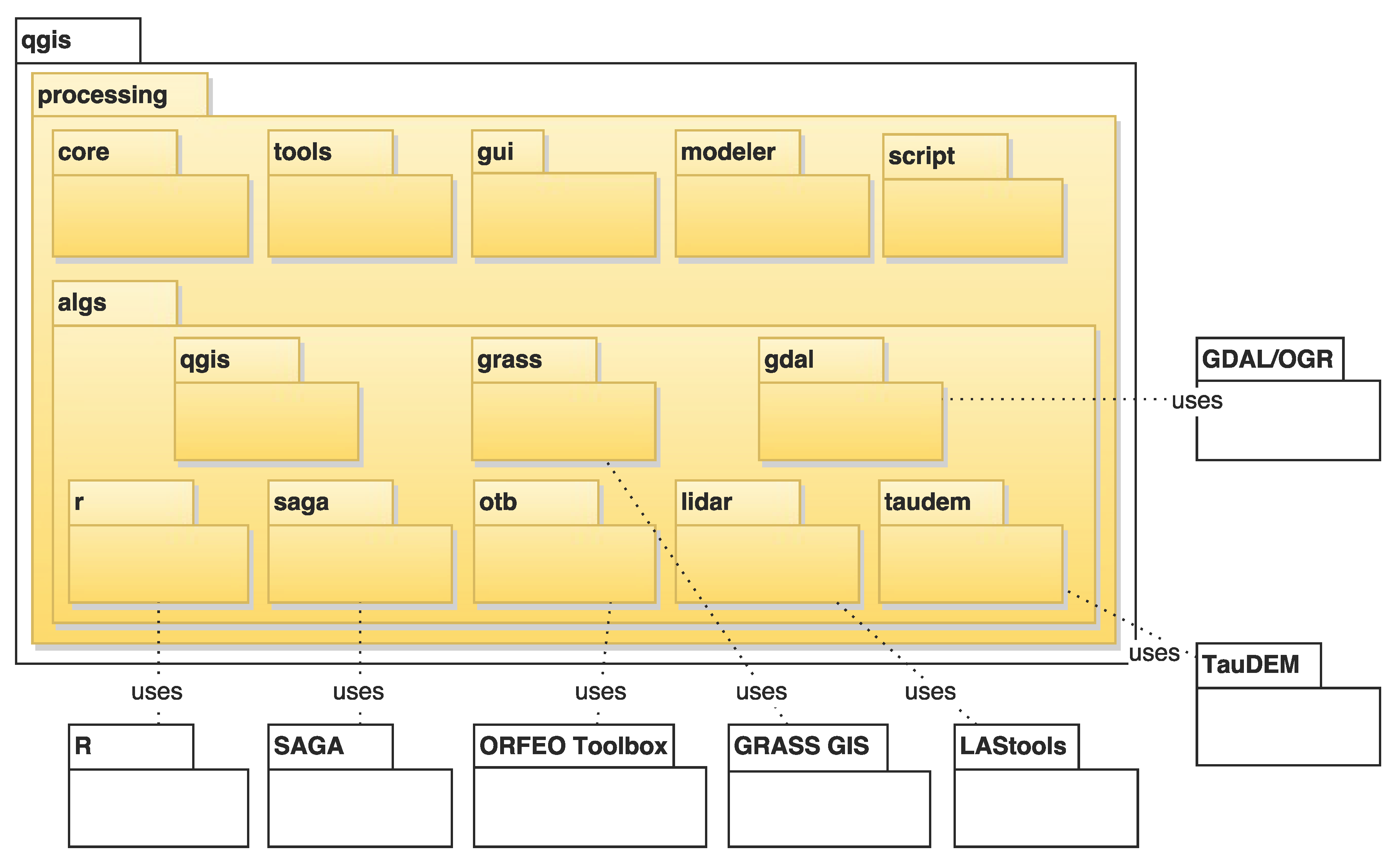
Figure 1 provides an overview of the packages that make up Processing and their interactions with external libraries. The following sections describe the Processing package content and the interactions of the contained classes in detail.

Figure 1. Package diagram with Processing packages (highlighted in yellow) and related packages.

Figure 1. Package diagram with Processing packages (highlighted in yellow) and related packages.

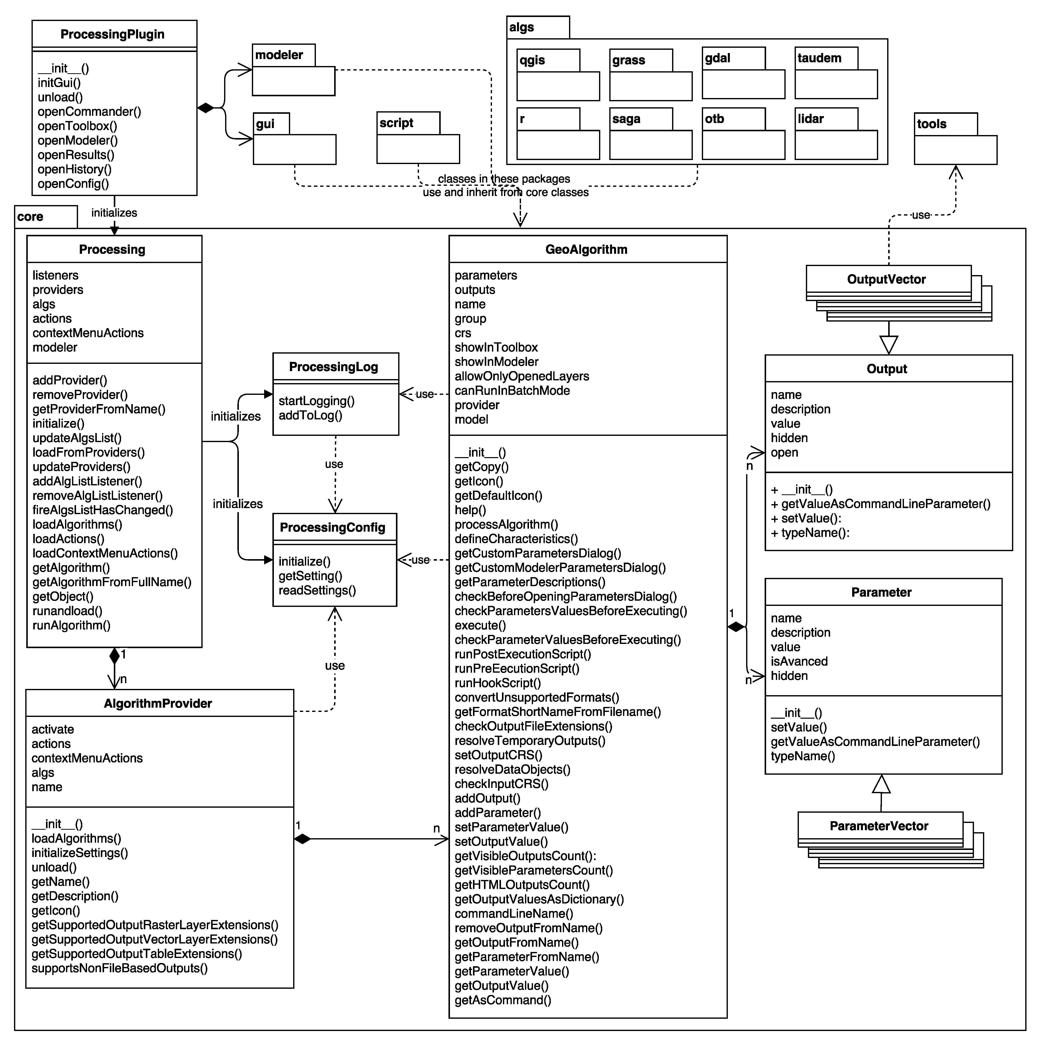
The core package contains the central classes of the Processing framework. Figure 2 shows the most important classes in this package (please note that for reasons of clarity, as well as to stay within the restrictions of the paper format, we do not show every error, output, parameter or GUI class in the following class diagrams). When the plugin is loaded, the ProcessingPlugin instance initializes the core Processing class. This in turn initializes the ProcessingConfig and ProcessingLog and loads the configured AlgorithmProviders. Each AlgorithmProvider contains a list of GeoAlgorithms, which contain the logic for geospatial analysis algorithms, such as the required Parameters and Outputs.

More specifically, the implementation of algorithms in the GeoAlgorithm class involves two main steps: first, the inputs required by the algorithm and the outputs that it will produce are specified. These should be included in the defineCharacteristics() method, which populates the arrays of inputs and outputs, defining the semantics of the algorithm. Additional parameters that describe the algorithm, such as the name of the associated group, are also defined in this method. In some cases, for example, where algorithms use a backend, such as GRASS or SAGA, parameters are not directly defined in these methods. Instead, defineCharacteristics() reads the input and output descriptions from a file and uses that information to populate the input and output arrays. This is done to simplify the process of adding the large collections of algorithms that these backends provide by taking advantage of the fact that most of them provide some mechanism of describing their algorithms. This makes is easier to adapt to new versions of the backend software, where algorithms might have changed, since the necessary adaptations are limited to changes in the description files and no Processing code has to be rewritten.

Figure 2. Class diagram of the core package and its connection to other packages.

Figure 2. Class diagram of the core package and its connection to other packages.

As the second step, the algorithm code, which will use the inputs provided to the algorithms and produce the outputs, is implemented in the processAlgorithm() method. This method must take the values of the algorithm input parameters (which have been set by the user through any of the UI elements of processing, such as the toolbox, batch processing interface, etc.) to compute outputs. Outputs are stored in the locations specified by the user-defined output configuration (at the moment, only file output is supported). Once the algorithm is implemented, it is added to the list of available algorithms. Processing can then setup the algorithm, prepare the input datasets, execute the algorithm and later process the resulting outputs. When the algorithm is executed, Processing runs the processAlgorithm() method, along with ancillary methods, which check the integrity of the input and output configuration, resolve output names (in the case of using temporary outputs, in which Processing itself sets the output file path), among other tasks needed to ensure the correct execution. Specific algorithm implementations in the different subpackages of the algs package will be discussed in the respective sections.

Besides core, the tools package contains essential utility functions and classes, which are used by other packages. Utility functions include alglist(), which returns the full list of available algorithms. Similarly, alghelp() displays the algorithm help text and parameter descriptions, and runalg() runs the algorithm. See Listing 1 for usage examples.

Listing 1: Syntax of important utility functions of the tools package (for usage examples see https://docs.qgis.org/2.8/en/docs/user_manual/processing/console.html)

import processing
processing.alglist()
processing.alghelp(name_of_the_algorithm)
processing.runalg(name_of_the_algorithm, param1, param2, ..., paramN,
                  Output1, Output2, ..., OutputN)

3.1. Graphical User Interface

Processing algorithms can be used by any of the framework’s graphical user interface elements. The following GUI elements are currently implemented in the gui and modeler packages, as depicted in Figure 3 and Figure 4, respectively:

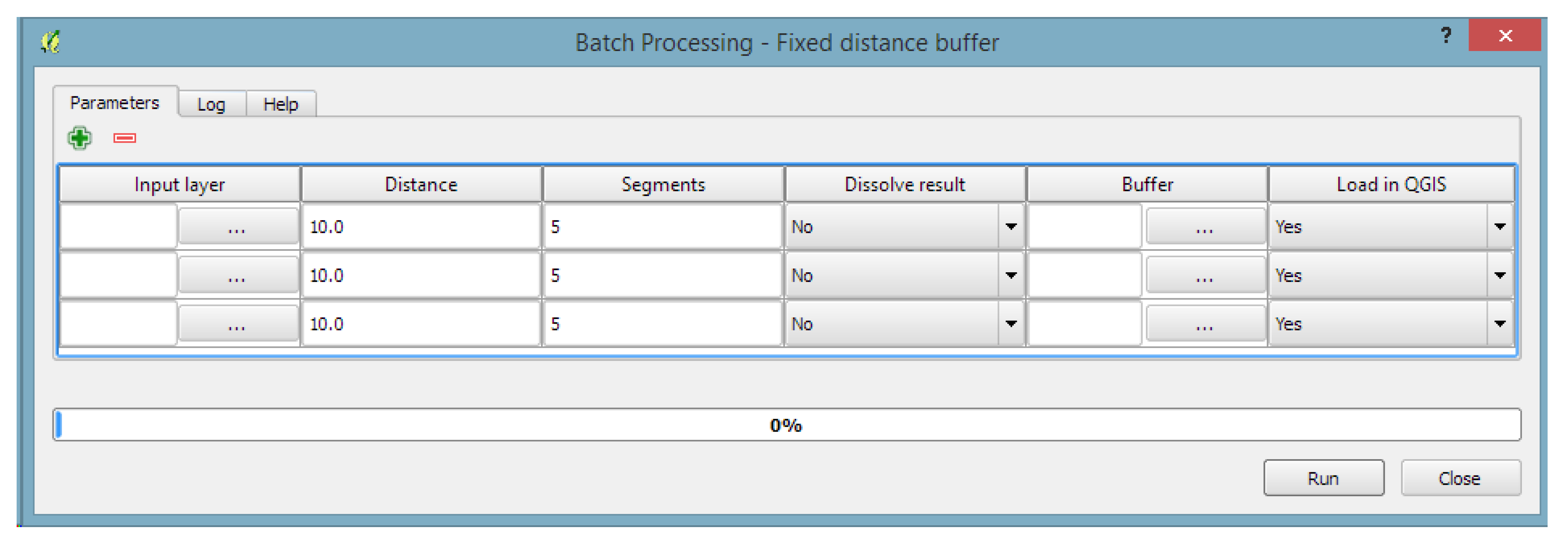
• The Toolbox (the gui.ProcessingToolbox class; for an example, see Figure 5) lists all available algorithms in its algorithmTree and allows one to execute algorithms and models using the AlgorithmDialog or BatchAlgorithmDialog. While the AlgorithmDialog is used to execute an algorithm or model once, the BatchAlgorithmDialog (for an example, see Figure 6) enables the repeated execution of an algorithm or model with varying parameter settings. The toolbox furthermore implements a mechanism that provides so-called Actions. This mechanism enables providers to extend the functionality of the toolbox and to provide tools that the provider needs. An example of this is the Create new script action that is added by the R provider, which opens a dialog for editing R scripts.
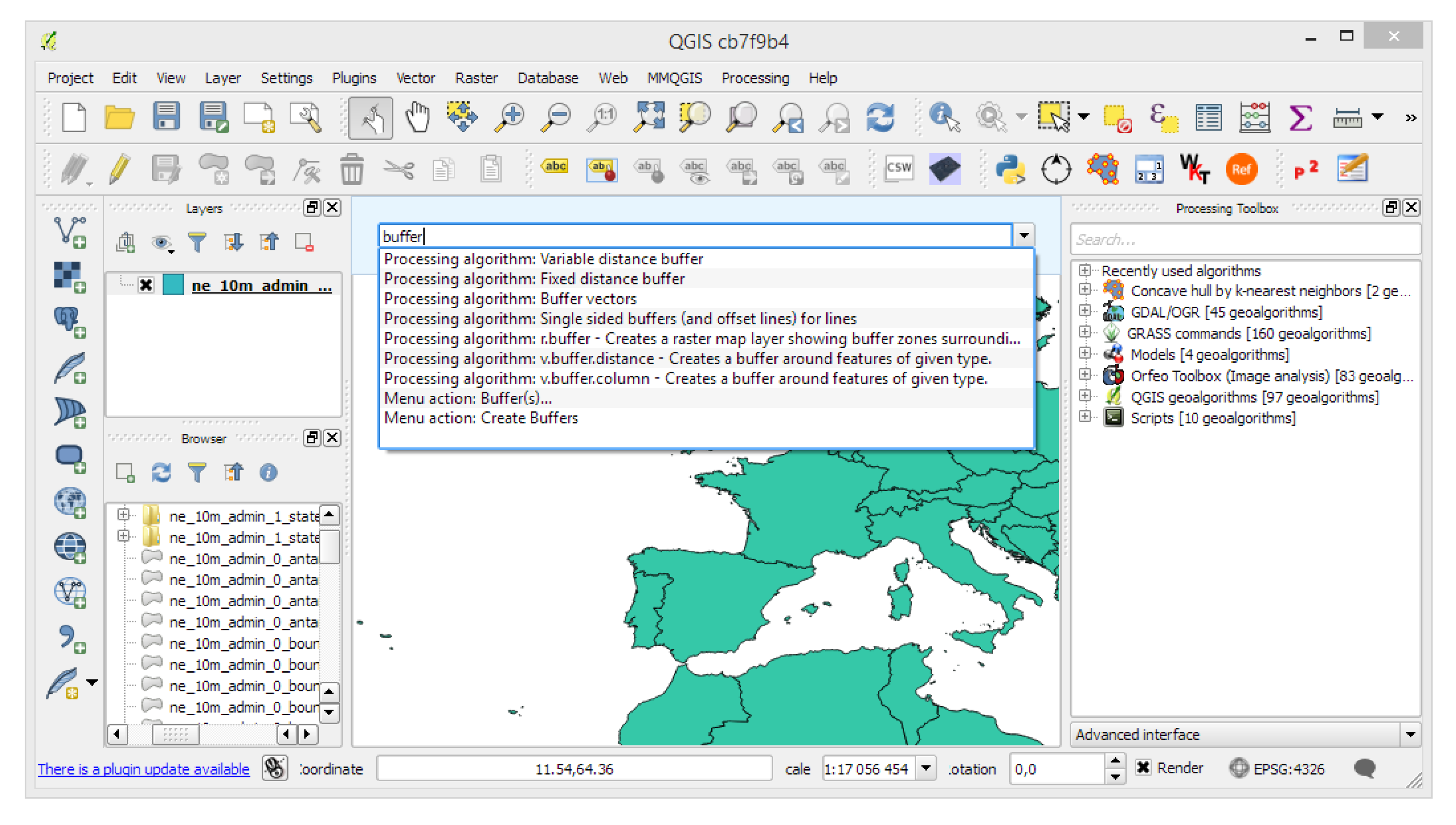
• The Commander (the gui.CommanderWindow class; for an example, see Figure 5) provides quick access to algorithms and models through a quick launcher interface. This enables the user to find and launch a geoprocessing tool by starting to type its name and picking the tool from the suggested search results.
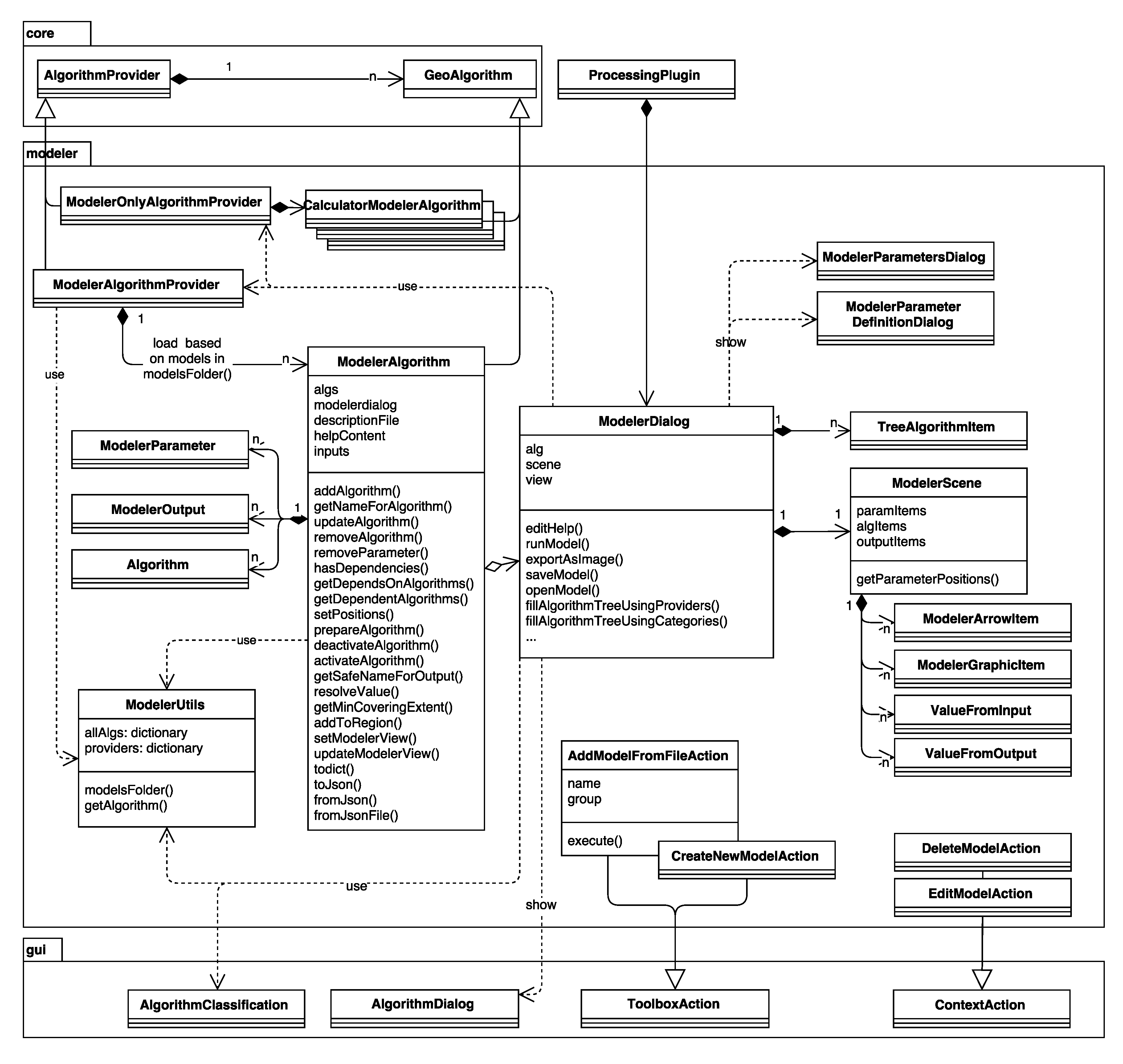
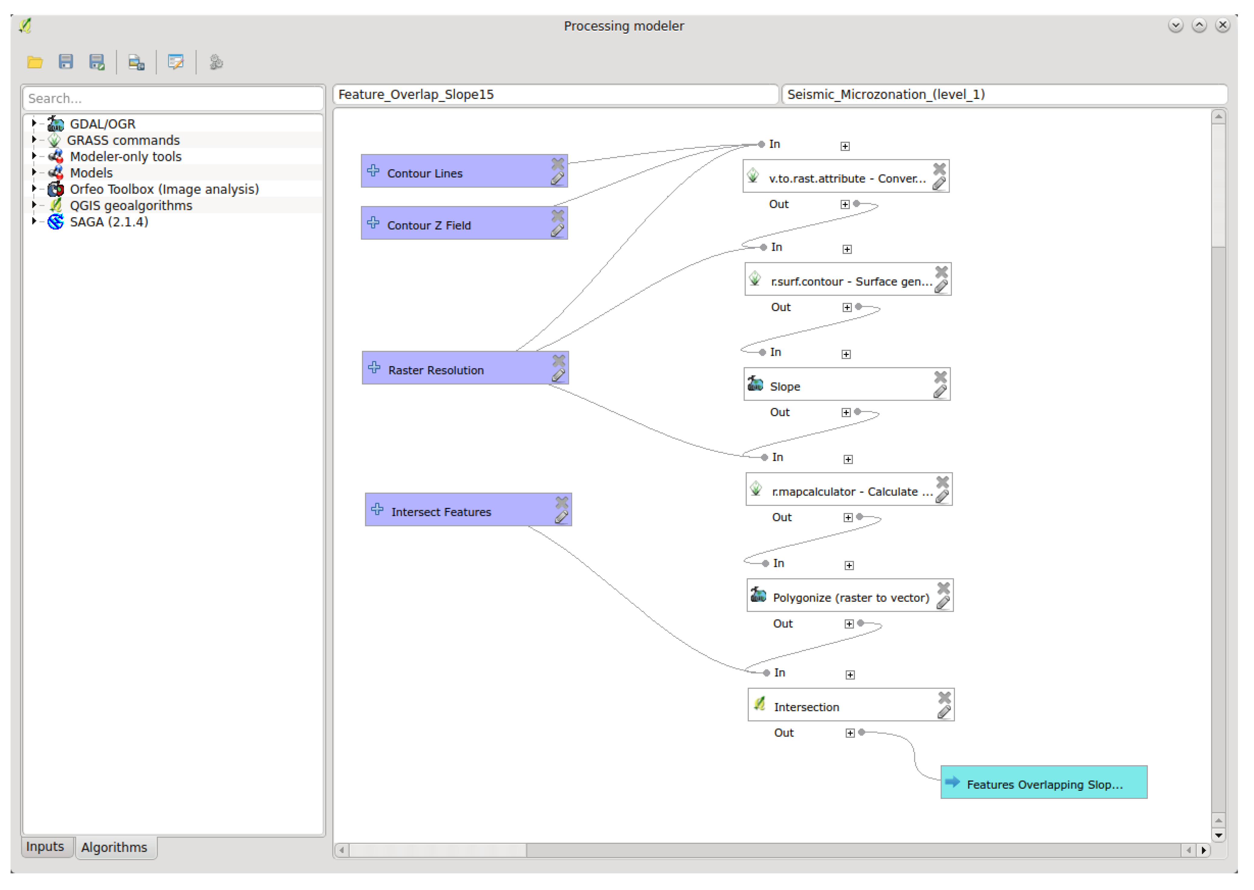
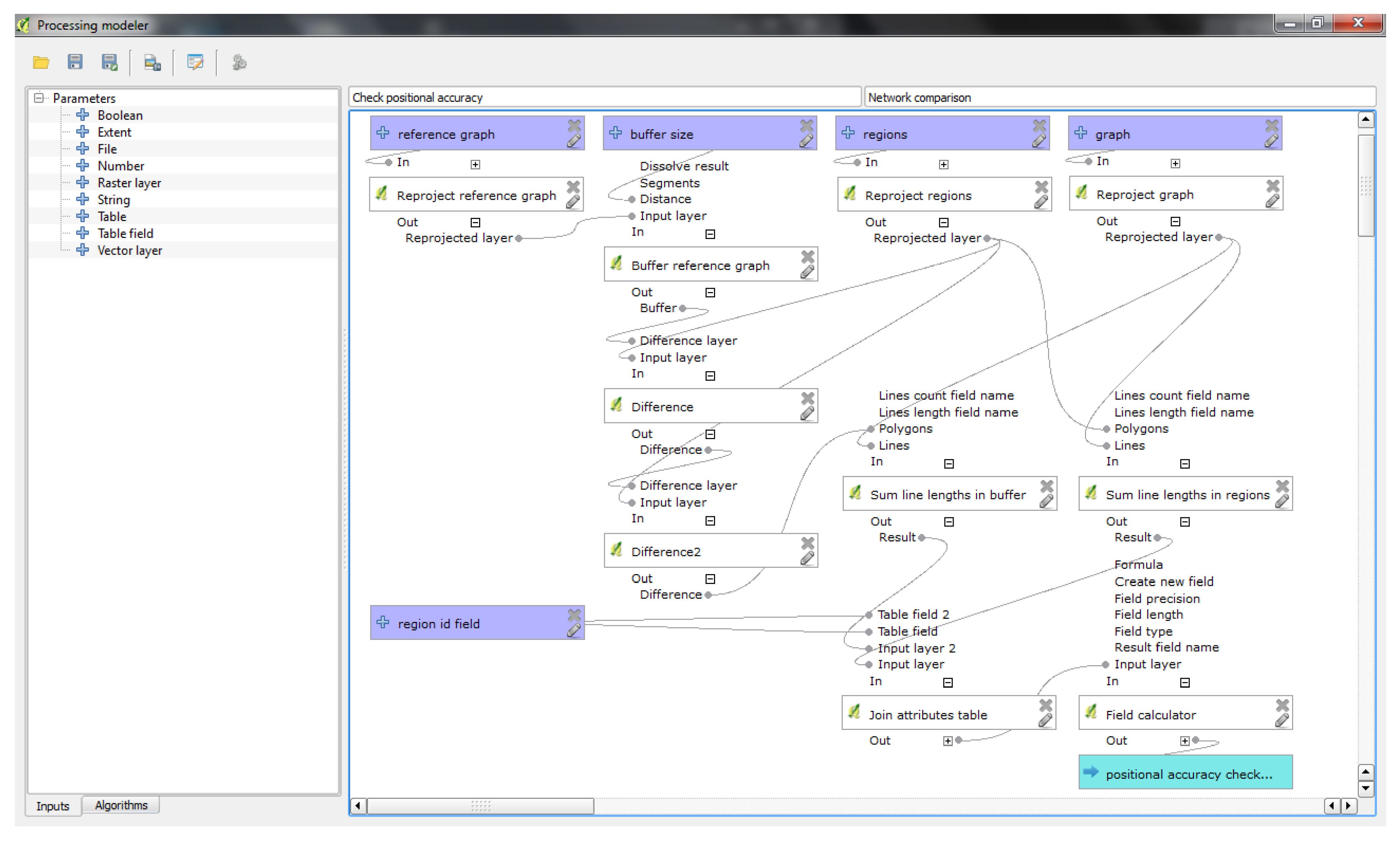
• The Graphical modeler (the modeler.ModelerDialog class; for examples, see Figure 7 and Figure 8) enables workflow automation by chaining individual tools into geoprocessing models. The visual representation of the model is drawn in the ModelerScene and consists of ModelerGraphicItems represented as boxes for input ModelParameters, Algorithms and ModelerOutputs, as well as ModelerArrowItems connecting them. The available input options and algorithms are listed in tree widgets similar to the one in the toolbox.

Figure 3. Class diagram of the gui package and its connections to other packages.

Figure 3. Class diagram of the gui package and its connections to other packages.

Customization of the graphical user interface associated with each algorithm is possible, both for execution from the toolbox, as well as for using the algorithm as part of a model. If no custom interface is provided, Processing creates the interface automatically. This is the case for most algorithms. To create the GUI, Processing uses the input and outputs of the algorithm, as defined in the algorithm description method. Depending on the data type of the input or output, the corresponding widget is selected, and all of them are arranged together in a simple AlgorithmDialog.

It is worth noting that models are instances of the ModelerAlgorithm class, which derives from the core GeoAlgorithm class. This way, Processing can treat models like any other algorithm, and it is possible to use both algorithms and existing models to build new models.

The following sections describe how Processing integrates algorithms from different analytical applications, such as QGIS ftools, MMQGIS, GDAL/OGR, SAGA, GRASS GIS, R and ORFEO Toolbox. These applications are supported by Processing out of the box. Further applications that are integrated in Processing by default, but are discussed only briefly in Section 3.7 due to their limited scope are TauDEM and Lastools. Finally, we show how new custom algorithms can be added and discuss the current limitations of the Processing framework.

Figure 4. Class diagram of the modeler package and its connections to other packages.

Figure 4. Class diagram of the modeler package and its connections to other packages.

Figure 5. Processing Toolbox (right panel) and Commander with auto-complete (top center).

Figure 5. Processing Toolbox (right panel) and Commander with auto-complete (top center).

Figure 6. Processing Batch processing GUI.

Figure 6. Processing Batch processing GUI.

Figure 7. Model for the creation of Level 1 seismic microzonation maps as used for [15] and described in [16].

Figure 7. Model for the creation of Level 1 seismic microzonation maps as used for [15] and described in [16].

Figure 8. Positional accuracy comparison model; updated version of the model published in [17].

Figure 8. Positional accuracy comparison model; updated version of the model published in [17].

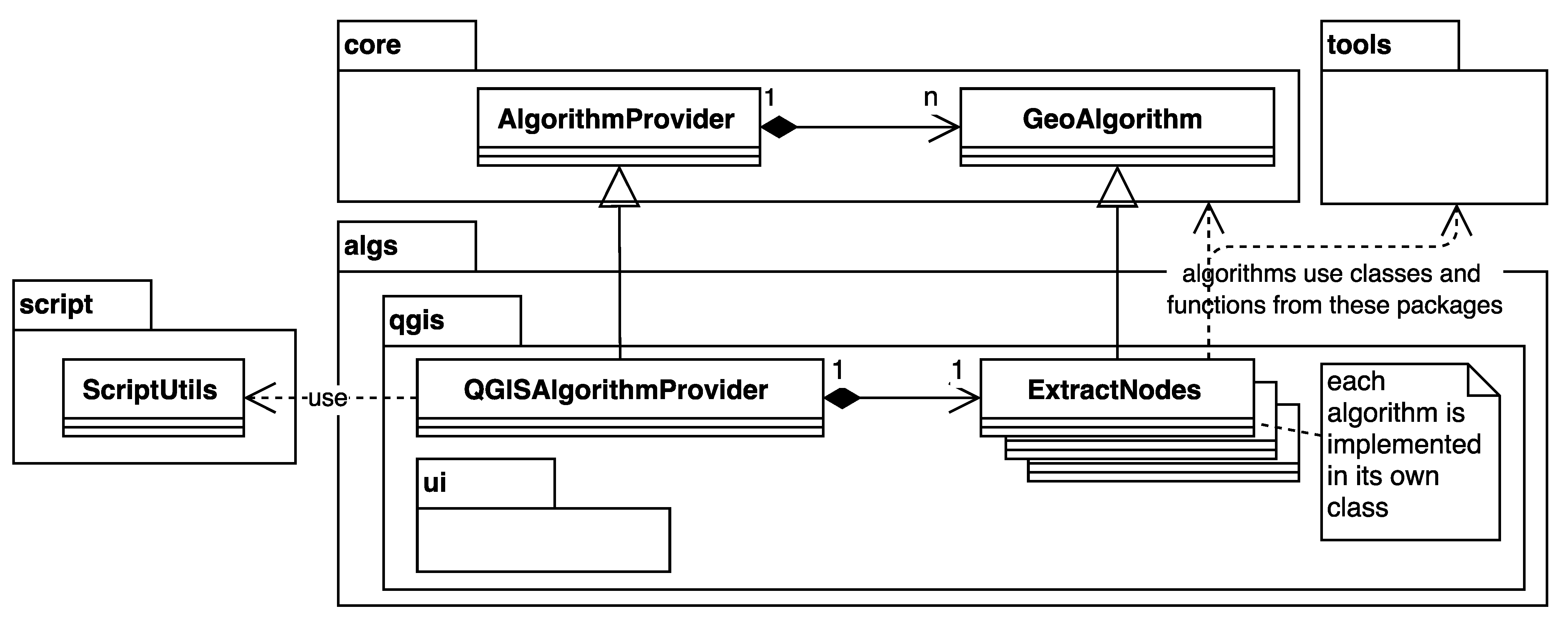
Figure 9. Class diagram of the qgis package and its connections to other packages.

Figure 9. Class diagram of the qgis package and its connections to other packages.

3.2. QGIS Ftools and MMQGIS Integration

ftools and MMQGIS [18] are two algorithm collections focusing on vector geoprocessing tools, which are provided as QGIS plugins. The algorithms from these collections were manually converted to Processing algorithms and are organized in the qgis package, as illustrated in Figure 9. This was achieved by adapting the tool code to the specific format of the GeoAlgorithm class, which is the base for all Processing algorithms.

Listing 2: Implementation of the ftools Extract nodes tool (shortened, for the full script see https://github.com/qgis/QGIS/blob/master/python/plugins/processing/algs/qgis/ExtractNodes.py)

from qgis.core import QGis, QgsFeature, QgsGeometry
from processing.core.GeoAlgorithm import GeoAlgorithm
from processing.core.parameters import ParameterVector
from processing.core.outputs import OutputVector
from processing.tools import dataobjects, vector
class ExtractNodes(GeoAlgorithm):
   INPUT = ’INPUT’
   OUTPUT = ’OUTPUT’
   def defineCharacteristics(self):
      self.name = ’Extract nodes’
      self.group = ’Vector geometry tools’
      self.addParameter(ParameterVector(self.INPUT,
         self.tr(’Input layer’),
         [ParameterVector.VECTOR_TYPE_POLYGON,
         ParameterVector.VECTOR_TYPE_LINE]))
      self.addOutput(OutputVector(self.OUTPUT,
         self.tr(’Output layer’)))
   def processAlgorithm(self, progress):
      layer = dataobjects.getObjectFromUri(
         self.getParameterValue(self.INPUT))
      writer = self.getOutputFromName(self.OUTPUT)
         .getVectorWriter(
            layer.pendingFields().toList(),
            QGis.WKBPoint, layer.crs())
      outFeat = QgsFeature()
      outGeom = QgsGeometry()
      for f in vector.features(layer):
          points = vector.extractPoints(f.geometry())
          outFeat.setAttributes(f.attributes())
          for i in points:
	 outFeat.setGeometry(outGeom.fromPoint(i))
              writer.addFeature(outFeat)
      del writer

These tools make extensive use of the QGIS Python API and the geoprocessing algorithms implemented in the QGIS core application. Listing 2 shows a shortened version of the Processing implementation of the ftools Extract nodes tool. This example illustrates how the new algorithm extends the GeoAlgorithm class and implements the two methods defineCharacteristics() and processAlgorithm(), which, respectively, describe and run the algorithm.

3.3. GDAL/OGR Integration

GDAL (Geospatial Data Abstraction Library) is a translator library for raster and vector geospatial data formats. Traditionally, GDAL used to focus on the raster part of the library and OGR the vector part for simple features. Starting with GDAL 2.0, both parts have been integrated more tightly. Multiple applications, such as QGIS, use this library for reading and writing spatial data. It implements a single raster abstract data model and vector abstract data model for all supported formats. Additionally, GDAL comes with a variety of command line utilities for data translation and processing [19].

The GdalOgrAlgorithmProvider integrates GDAL-based algorithms into the Processing framework, as illustrated in Figure 10. Individual algorithms extend the GdalAlgorithm or OGRAlgorithm class and have been implemented using two different mechanisms: calling the GDAL/OGR Python bindings or using the GDAL command line interface.

Figure 10. Class diagram of the gdal package and its connections to other packages.

Figure 10. Class diagram of the gdal package and its connections to other packages.

When GDAL/OGR Python bindings exist for a function, the corresponding GdalAlgorithm or OGRAlgorithm calls GDAL/OGR, as shown in the example in Listing 3, which uses GDAL to extract projection information from an input file.

Listing 3: Integration of Extract projection using GDAL Python bindings (shortened, for the full script see https://github.com/qgis/QGIS/blob/master/python/plugins/processing/algs/gdal/extractprojection.py)

from osgeo import gdal, osr
from processing.algs.gdal.GdalAlgorithm import GdalAlgorithm
...
class ExtractProjection(GdalAlgorithm):
   ...
   def processAlgorithm(self, progress):
      rasterPath = self.getParameterValue(self.INPUT)
      createPrj = self.getParameterValue(self.PRJ_FILE)
      raster = gdal.Open(unicode(rasterPath))
      crs = raster.GetProjection()

Listing 4: Integration of Clip raster by extent using the command line interface (shortened, for the full script see https://github.com/qgis/QGIS/blob/master/python/plugins/processing/algs/gdal/ClipByExtent.py)

from processing.algs.gdal.GdalAlgorithm import GdalAlgorithm
from processing.algs.gdal.GdalUtils import GdalUtils
...
class ClipByExtent(GdalAlgorithm):
   ...
   def processAlgorithm(self, progress):
      out = self.getOutputValue(self.OUTPUT)
      noData = str(self.getParameterValue(self.NO_DATA))
      projwin = str(self.getParameterValue(self.PROJWIN))
      extra = str(self.getParameterValue(self.EXTRA))
      arguments = []
      arguments.append(’-of’)
       arguments.append(GdalUtils.getFormatShortNameFromFilename(out))
      ...
      regionCoords = projwin.split(’,’)
      arguments.append(’-projwin’)
      arguments.append(regionCoords[0])
      arguments.append(regionCoords[3])
      arguments.append(regionCoords[1])
      arguments.append(regionCoords[2])
      ...
      GdalUtils.runGdal([’gdal_translate’,
         GdalUtils.escapeAndJoin(arguments)], progress)

Other algorithms, such as warp, translate, contour or clipping (see Listing 4), are called directly using the command line interface. All algorithms in the GDAL provider that call GDAL tools on the command line rely on the GdalUtils.runGdal() method. This method takes care of preparing the command line based on the parameter values, as well as the platform being used. It also handles the output created by the GDAL algorithms and provides progress indication and logging of output content.

3.4. SAGA and GRASS GIS Integration

SAGA and GRASS have been integrated in Processing in a similar manner; therefore, their integration is described together in this shared section.

The System for Automated Geoscientific Analyses (SAGA) is a GIS focusing on spatial data processing and analysis [13]. SAGA functions are organized as modules in framework-independent module libraries and can be accessed via SAGA’s graphical user interface or various scripting environments, such as shell scripts, Python or R [20].

The Geographic Resources Analysis Support System (GRASS GIS) is a multi-purpose open source GIS [21]. It supports 2D and 3D raster and vector data and includes vector network analysis functions, spatial modeling algorithms, 3D visualization, as well as image processing routines pertaining to LiDAR and multi-band imagery [4].

Figure 11. Class diagram of the saga package and its connections to other packages.

Figure 11. Class diagram of the saga package and its connections to other packages.

Both SAGA and GRASS GIS offer a great number of algorithms, and their executables are included in most QGIS packages, so there is no need to install them separately to have this functionality available. Although both SAGA and GRASS GIS can be called from Python using their corresponding Python APIs, Processing uses their command line interfaces, since these have proven to provide more stability (at least at the time of the initial implementation) and allowed for a quicker implementation of a large number of algorithms. 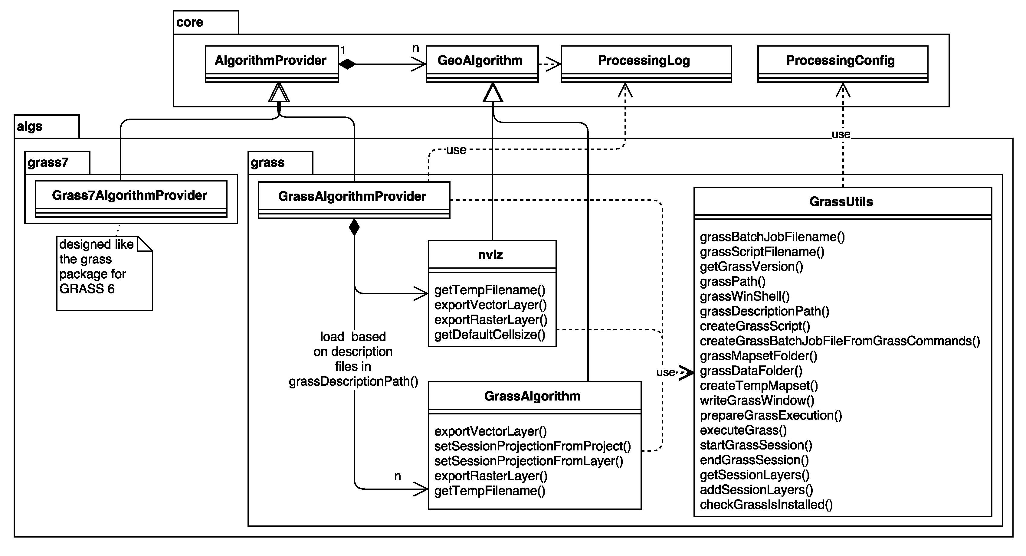As shown in Figure 11, Processing currently supports SAGA Versions 2.1.2, 2.1.3 and 2.1.4 through the SagaAlgorithm212, SagaAlgorithm213 and SagaAlgorithm214 classes implemented in the saga package, respectively. Similarly, GRASS 6 and 7 are supported through the grass and grass7 packages, as shown in Figure 12.

Figure 12. Class diagram of the grass and grass7 packages and their connections to other packages.

Figure 12. Class diagram of the grass and grass7 packages and their connections to other packages.

More specifically, SAGA and GRASS GIS integration is achieved using four main steps: description of algorithm inputs and outputs, input data preparation, algorithm execution and output handling.

Listing 5: Algorithm description for GRASS v.voronoi (as given in https://github.com/qgis/QGIS/blob/master/python/plugins/processing/algs/grass/description/v.voronoi.txt)

v.voronoi
v.voronoi - Creates a Voronoi diagram from an input vector layer
            containing points.
Vector (v.*)
ParameterVector|input|Input points layer|0|False
ParameterBoolean|-l|Output tessellation as a graph (lines),not areas
   |False
ParameterBoolean|-t|Do not create attribute table|False
OutputVector|output|Voronoi diagram

Descriptions of the algorithm inputs and outputs are necessary to automatically create the GUI, run the algorithm, as well as to know which outputs will be generated. This information is stored in a separate file for each algorithm. The location of these description files can be accessed using SagaUtils.sagaDesriptionPath() and GrassUtils.grassDescriptionPath(), respectively. Both SAGA and GRASS provide methods to describe their algorithms. These methods simplify the integration, since it is not necessary to create the algorithm description files manually. Listing 5 shows an example description for the GRASS GIS v.voronoi algorithm, which features one input and one output, as well as two configuration parameters.

The second integration step is the preparation of the input datasets. This is necessary since SAGA and GRASS GIS use their own formats for vector and raster data, and layers in popular formats that are supported by QGIS cannot be directly used by them. Therefore, Processing takes care of converting layers into the required formats before calling the algorithm. This provides a seamless integration into QGIS, allowing the user to use data, even if it is stored in a format that is not natively supported by SAGA or GRASS GIS. Additionally, in the case of vector layers, the data conversion can also make SAGA and GRASS GIS aware of feature selections by converting only the selected features before calling the algorithm.

In the third integration step, the algorithm is executed using either the original input layer (if the data type is natively supported) or the converted layers.

The final and fourth integration step is the handling of outputs. Processing receives the output generated by SAGA/GRASS GIS and adds it to the current QGIS project. If the output format specified by the user is not supported by SAGA/GRASS GIS, Processing will take care of converting the output before loading the layer. For instance, SAGA does support conversion from its native raster format into TIFF format, but cannot produce a TIFF file directly. Therefore, if the user specifies a TIFF output, it is necessary to first create a native SAGA raster layer, which can then be converted to TIFF by calling the SAGA conversion algorithm.

Depending on the format, data conversions for both input and output are performed using functions provided by QGIS or the external application. Conversions using SAGA/GRASS GIS require several calls to the application. Therefore, all calls necessary to convert data and run the algorithm are written to a script file using SagaUtils.createSagaBatchJobFileFromSagaCommands() and GrassUtils.createGrassBatchJobFileFromGrassCommands(), respectively, which is then executed in one go.

3.5. R Integration

R is a system for statistical computation and graphics. It consists of a language plus a run-time environment to run programs stored in script files [22]. The R project also provides packages, functions, classes and methods for handling spatial data [23].

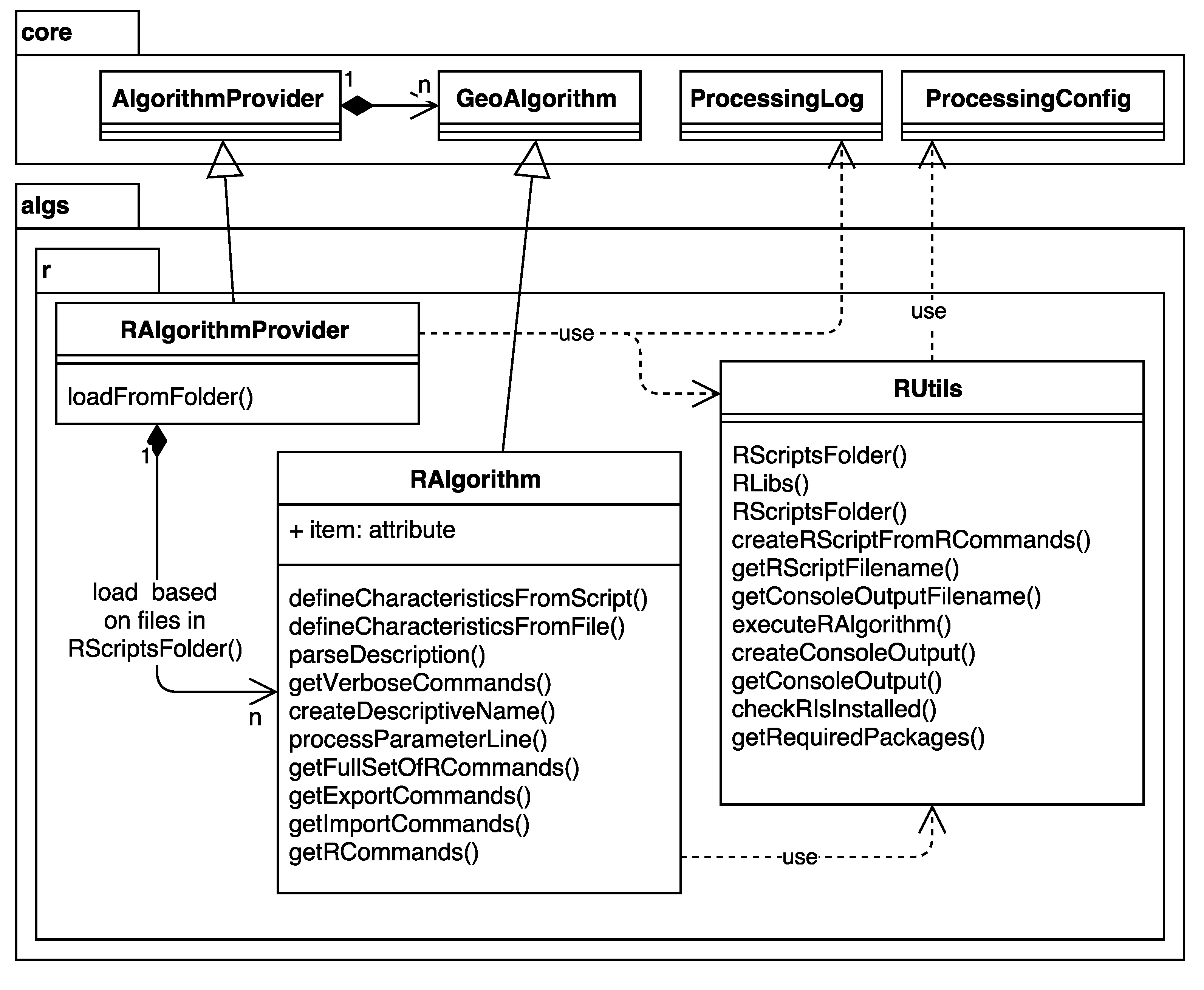
Processing integrates R into QGIS, enabling users to run R scripts from within QGIS and use QGIS layers as inputs. Figure 13 shows the classes of the r package. Similar to the SAGA/GRASS GIS integration, R integration includes data conversion routines for inputs and outputs, and it runs R on the command line using RUtils.executeRAlgorithm(). The main difference is that the RAlgorithmProvider does not offer any predefined algorithms. Instead, it enables the users to create their own algorithms, which can be written using a built-in text editor and can be stored and used in future sessions. The location of the R scripts can be accessed using RUtils.RScriptsFolder().

R scripts in Processing use the standard R syntax extended by additional header elements (represented by code lines starting with double hashes ##), which provide the information Processing needs to understand the context, as well as the inputs and outputs of the algorithms. An example using R to compute and display a histogram is given in Listing 6.

3.6. ORFEO Toolbox Integration

The ORFEO Toolbox (OTB) is a library of image processing algorithms, which is based on the medical image processing library Insight Segmentation and Registration Toolkit (ITK) . It provides functionality for remote sensing image processing in general and for high spatial resolution images in particular [24].

Figure 13. Class diagram of the R package and its connections to other packages.

Figure 13. Class diagram of the R package and its connections to other packages.

Listing 6: Processing R script for the R Histogram function (as given in in https://github.com/qgis/QGIS/blob/release-2_8/python/plugins/processing/algs/r/scripts/Histogram.rsx

##Vector processing=group
##showplots
##Layer=vector
##Field=Field Layer
hist(Layer[[Field]], main=paste("Histogram of",Field),
     xlab=paste(Field))

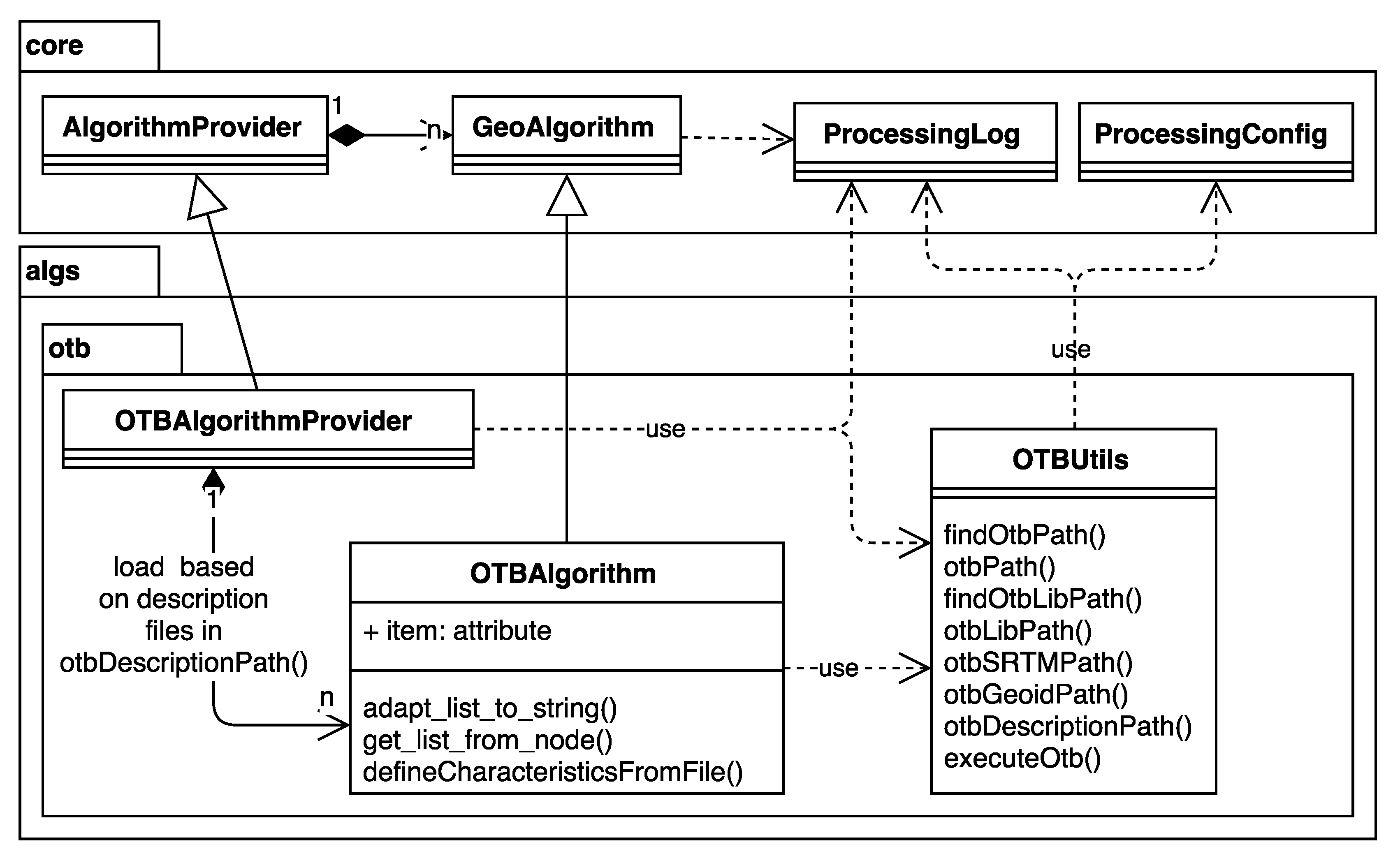
Figure 14 shows the classes of the otb package. The integration of OTB into Processing is similar to that of SAGA and GRASS GIS, since it calls the corresponding command line tools, which are located in the OTBUtils.otbDescriptionPath() and then loads the output images generated by them. To simplify the execution of certain algorithms that require similar parameters, some of those parameters have been added to the OTBAlgorithmProvider configuration settings, so that they can be configured once and then be used automatically whenever an algorithm that requires them is run. In particular, the SRTM (Shuttle Radar Topography Mission) tiles folder parameter (which can be accessed using OTBUtils.otbSRTMPath()) and the geoid file parameter (which can be accessed using OTBUtils.otbGeoidPath()) will be used by default in the parameters dialog of an OTB algorithm that uses any of them.

Figure 14. Class diagram of the otb package and its connections to other packages.

Figure 14. Class diagram of the otb package and its connections to other packages.

3.7. Integration with Other Backends

Algorithm providers that integrate other backends, such as LWGEOM, are available, as well. However, these providers are not part of Processing itself and exist as independent plugins that work on top of Processing, taking advantage of its modular and pluggable architecture.

The TauDEM provider represents a special case. TauDEM (Terrain Analysis Using Digital Elevation Models) is a suite of digital elevation model (DEM) tools for the extraction and analysis of hydrological information from topography as represented by a DEM [25]. The TauDEM provider is a core provider due to historical reasons. It was added to Processing when the framework itself was still in development, and it has been kept there despite being highly specific rather than of general interest.

A similar situation is found in the case of the LiDAR provider, which provides a frontend for two popular tools for working with LiDAR data: LAStools and Fusion. Although part of the core Processing distribution, these providers are disabled by default, as they require backends that need to be installed separately and are not included in the most common QGIS distributions.

The number of QGIS plugins that extend Processing with new providers is growing, and most of them use techniques similar to the ones described in the above sections. Those providers are, however, not described here. The following section describes this expanding Processing with new providers, as well as other available options.

3.8. Development of New Algorithms

New algorithms can be integrated into Processing using three different techniques, with increasing complexity: writing a Python Processing script, creating a new QGIS plugin, which implements a Processing provider, or adding new classes to the Processing core.

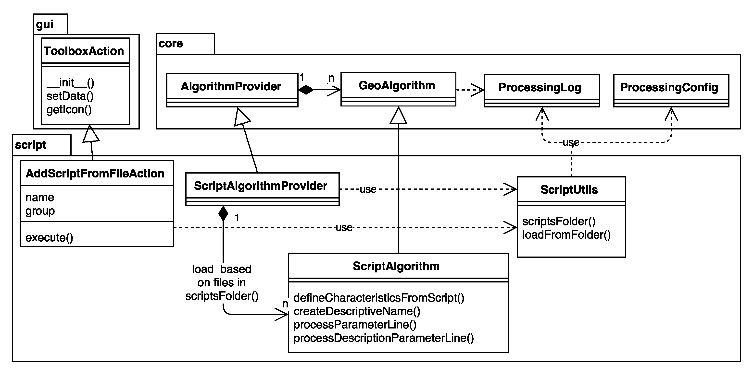
Creating a python script is the most straight-forward way to add new algorithms to Processing. These scripts are handled by the script package depicted in Figure 15. Scripts are simple to create, since they can be written directly in QGIS, using the built-in editor. This is the recommended approach for most cases. Users can share scripts and associated documentation (in .help files) on a dedicated Github repository [26], and other users can download these tools using the built-in “Get scripts/models from online source” functionality. The location of the scripts can be accessed using ScriptUtils.scriptsFolder().

Figure 15. Class diagram of the script package and its connections to other packages.

Figure 15. Class diagram of the script package and its connections to other packages.

Listing 7 shows an example script, which increments the value in the given input field of the input vector layer by one and outputs the result as a new vector layer. The first three lines marked by double hashes ## contain the input and output configuration. The remainder of the script performs the data processing. This example also serves to show how Processing supports efficient implementation by providing easy to use functions, such as processing.getObject() to read the input data and the processing.core.VectorWriter class to save the results.

The second option is creating a new QGIS plugin, which implements a Processing provider. A provider wraps a set of algorithms, and it can be registered on the Processing framework, telling Processing to display its algorithms to the user. This allows one to create new stand-alone plugins that integrate with Processing. Their algorithms can be enabled or disabled by enabling or disabling the respective plugin using the QGIS plugin manager.

Listing 7: Example Processing script demonstrating script input and output configurationscript

##input=vector
##field=field input
##results=output vector
from qgis.core import *
from processing.core.VectorWriter import VectorWriter
layer = processing.getObject(input)
writer = VectorWriter(results, None, layer.pendingFields(),
                       layer.dataProvider().geometryType(),
                       layer.crs())
for feat in layer.getFeatures():
    feat.setAttribute(field, feat[field]+1)
    writer.addFeature(feat)
del writer

The most advanced third option is to add classes to the Processing core. This is restricted to core developers and not recommended for regular users.

3.9. Limitations

Processing has certain limitations, particularly when it comes to integrating external applications. This is mostly due to restrictions in the semantics of the algorithms, which in some cases make it difficult or impossible to create certain types of algorithms. The following limitations of the Processing framework for defining algorithms should be noted:

• Inputs and outputs are fixed, and optional parameters or outputs are not supported. This limitation was introduced deliberately in order to ensure correct working and efficient implementation of algorithm workflow support using Processing models. It is worth noting that the algorithm design, which handles the list of outputs and inputs, could easily accommodate optional parameters, but they would increase the complexity of Processing models. Therefore, restrictions were imposed when the GeoAlgorithm class was designed. There is currently no short- or medium-term plan to add support for optional parameters and outputs, since this might require a rewrite of the Modeler.
• Algorithms cannot have any type of interactivity and should work in a black box way, receiving inputs and providing output files without the user participating in the process. This limitation was introduced to ensure that models generated from Processing algorithms can run automatically without the need for user actions.
• Performance is reduced when the input dataset has to be converted. This is particularly noticeable with large datasets. Currently, Processing does not take advantage of the fact that it is not necessary to convert datasets when chaining several algorithms of the same provider. An optimization mechanism is currently under development.

In the particular case of the SAGA and GRASS GIS integration, these limitations have been handled manually, adapting those algorithms that could not be integrated directly in their current form or removing them in some cases. The following are some of the limitations of the SAGA integration:

• SAGA’s interactive algorithms, such as kriging with interactive variogram fitting, have not been added to Processing.
• Single algorithms implementing multiple methods with optional parameters were split into multiple Processing algorithms. This solution was used, for example, for the SAGA buffer algorithm, which was split into one Processing algorithm for each method with its respective parameters.
• SAGA support for vector data, when used on the command line, is limited to shapefiles. This leads to inconsistent results, especially when the original dataset contains field names longer than 10 characters, which are not supported by the DBF (dBASE database file) format used to store attribute data in shapefiles.

4. Use Cases and Application Examples

This section discusses typical geoprocessing use cases in research and development and how the design of Processing supports them. The presented use cases include automating and documenting geoprocessing workflows consisting of algorithms from one or more sources using models and scripts, implementing new algorithms, as well as sharing models or scripts to facilitate reproducible research. The real-world application examples used to illustrate these use cases span the fields of ecology, data quality assessment, mobility research, risk assessment and geology.

4.1. Workflow Automation and Documentation

A core use case of the Processing framework is workflow automation. By automating workflows, users can increase their efficiency by reducing time spent on repetitive tasks. Additionally, models and scripts can also serve as a means to document workflow steps. Automation can be achieved by chaining tools in geoprocessing models or by calling algorithms in Python scripts.

Workflow automation using geoprocessing models is used, for example, by [27], who use a model combining SAGA and GDAL algorithms to create a hydrological network for their assessment of the effects of forest certification on the ecological condition of Mediterranean streams. While both SAGA and GDAL algorithms could also be accessed from the command line, the possibility of integrating algorithms from both sources in a graphical model enables the researcher to focus fully on the actual analysis, rather than having to deal with the particularities and command line syntax of the involved tools.

Further examples of Processing model applications can be found in the QGIS case study section: [28] presents a model to map hotspot areas for biodiversity and ecosystem services, which combines GRASS GIS, SAGA and QGIS tools; [29] presents a model to compute forest fire risk, which combines GRASS GIS, SAGA and QGIS tools (more specifically, QGIS ftools and MMQGIS). Most recently, [16] presented a model to automate the identification of unstable seismic zones combining GRASS GIS, GDAL and QGIS algorithms, as depicted in Figure 7.

To further automate spatial analyses, Processing scripts and models can be called from the command line and within Python scripts. For example, [30] developed a Processing script that computes energy estimates for electric vehicles on a certain route. To compare the influence of different input datasets and parameter settings, they employ a Python script that handles calling the Processing script with different combinations of input datasets and parameter settings. Listing 8 shows a simplified version of the script, which illustrates how user-generated Processing scripts (such as the estimateenergy script) and other Processing tools (such as qgis:basicstatisticsfornumericfields) can be called using processing.runalg() and their results used, in this example, to compute descriptive statistics.

Listing 8: Example usage of Processing on the command line (simplified version of the script used for [30])

import processing
out_path =  "/home/user/output.shp"
processing.runalg("script:estimateenergy",
   "input.shp","id","/home/user/input.tif",v, out_path)
stats = processing.runalg("qgis:basicstatisticsfornumericfields",
   out_path,"kWh",None)
avg_kwh = stats[’MEAN’]

4.2. Integration of New Algorithms

Processing facilitates the development of geoprocessing tools and adding new algorithms to the Toolbox by allowing researchers and developers to focus on the core algorithms while the automatic GUI generation and utility functions for accessing and writing data take care of the repetitive tasks. Integration of the new algorithm can be achieved by writing custom Processing scripts or by developing additional algorithm providers.

Integration of new algorithms using scripts is used, for example, by [17], who present geoprocessing models for OpenStreetMap data quality assessment, which combine existing tools from the Processing Toolbox and custom scripts created particularly for this task. The custom scripts include an implementation of Hausdorff distance computations (https://github.com/anitagraser/QGIS-Processing-tools/blob/master/1.1/scripts/hausdorff_distance_pairwise.py), which is used to determine the similarity of street network features in different datasets. This script takes advantage of Processing convenience tools, such as the VectorWriter class, to simplify writing the algorithm output. Furthermore, the user interface is generated automatically when the script is executed through the Toolbox or Modeler. The automatic GUI generation process takes care to, for example, only list vector layers as potential input layers and keep the input fields listing the layer attributes synced to the selected layers.

More examples of new algorithms can be found on the dedicated Github repository [26]. Users can access the documentation stored in the .help files through both the automatically-generated user interface, as well as the processing.alghelp(“algname”) function.

An example of a new algorithm provider is implemented in the Concave Hull plugin (http://plugins.qgis.org/plugins/concavehull/), which adds tools to cluster points and to compute concave hulls around sets of points. Besides this Processing integration, this plugin also offers a regular plugin user interface dialog, which can be accessed through the QGIS Vector menu. This approach enables the plugin developers to support both users who prefer classical plugin dialogs, as well as Processing users who might want to combine these tools with other tools in the Toolbox.

4.3. Sharing and Reproducible Research

Sharing geoprocessing tools (scripts, as well as models) is an important step towards reproducible research. Shared tools enable other researchers to study the analysis process and to reproduce the published results in a much more straight-forward fashion than by trying to reproduce the individual steps based on a textual description or having to implement the analysis from pseudocode.

For example, [17] describe a Processing model to assess the positional accuracy of the OpenStreetMap (OSM) street network by comparing it to a reference network. The workflow is based on a method described in [31], which has been applied in numerous other studies on OSM quality. The individual steps are easy to reproduce using standard GIS functionality, which certainly helped to make this method popular with many researchers. The model, which is shown in Figure 8, implements this method by combining multiple QGIS tools from the Processing Toolbox into one automatic workflow. The model can thus be applied to different areas of interest while ensuring that the process is always performed in the exact same way. Both the model diagram, as well as the model source code are published together with the paper (https://github.com/anitagraser/QGIS-Processing-tools/tree/master/1.1/models).

So far, sharing code has not yet become standard among researchers in the field of geographic information sciences and related disciplines using GIS. While some researcher publish at least diagrams of the Processing models they developed, many publications do not contain information at this level of detail. With the increasing trend towards reproducible research, we expect to see more Processing tools being published in the future.

5. Conclusions and Outlook

In this paper, we presented the Processing framework, which provides an efficient seamless integration of geoprocessing tools from a variety of sources into the QGIS geographic information system. This new framework was designed to overcome issues with previous implementations of geoprocessing tools in QGIS, such as the lack of user interface and behavior consistency, extensive code duplication and lack of automation capabilities. The Processing architecture avoids the need for duplication of development effort by directly integrating multiple libraries, such as QGIS, GDAL/OGR, SAGA, GRASS GIS, R and ORFEO Toolbox. Furthermore, Processing aims at facilitating both the development as well as the usage of geoprocessing tools.

For users, Processing makes it possible to automate geoprocessing tasks without the need for programming knowledge. It facilitates the usage of geoprocessing algorithms by automating input data format conversions where necessary and, thus, reduces potential error sources by reducing the number of manual steps the user has to perform.

For algorithm developers, Processing facilitates the development of new algorithms through automatic GUI generation for scripts and models. Furthermore, the Processing graphical modeler supports modular development of geoprocessing workflows, allowing each tool to focus on one clearly-defined functionality while complex workflows can be built by chaining specialized tools. Developers are encouraged to inspect all underlying code and to evaluate, benchmark, customize and enhance all algorithms and methods.

In research settings, Processing can facilitate reproducible research by enabling researchers to publish tools and models with their papers, which can be picked up directly by interested users to validate results or to apply the tools to their own data. The array of published applications demonstrates the wide applicability of the Processing framework.

In order to offer more flexibility for advanced modeling purposes, future development should add support for advanced features, such as conditional flows or loops in the graphical modeler. Another open issue is the implementation of alternatives to storing intermediate results or temporary files in shapefiles in order to avoid the drawbacks of this format, particularly the truncation of attribute names. Current enhancement plans include a Google Summer of Code project to add multi-threading support to Processing [32], as well as the integration of the spatial analysis library PySAL [33], as mentioned in [34].