Exploring Spatial Scale, Autocorrelation and Nonstationarity of Bird Species Richness Patterns

Abstract

In this paper we explore relationships between bird species richness and environmental factors in New York State, focusing particularly on how spatial scale, autocorrelation and nonstationarity affect these relationships. We used spatial statistics, Getis-Ord G_i*(d), to investigate how spatial scale affects the measurement of richness “hot-spots” and “cold-spots” (clusters of high and low species richness, respectively) and geographically weighted regression (GWR) to explore scale dependencies and nonstationarity in the relationships between richness and environmental variables such as climate and plant productivity. Finally, we introduce a geovisualization approach to show how these relationships are affected by spatial scale in order to understand the complex spatial patterns of species richness.

1. Introduction

The statistical methods used to relate biodiversity to environmental factors are essential for addressing a suite of ecological questions ranging from predicting the effects of climate change on biodiversity [1], identifying anthropogenic land cover changes on species richness [2], to exploring new locations for reserve sites [3]. Traditional studies investigating biodiversity have often explored the relationship between species richness (the number of different species recorded in a region) and a set of environmental factors at a single spatial scale [4,5,6,7]. The selection of the spatial scale when studying biodiversity is particularly pertinent, as factors and processes that are found to be important at one scale frequently prove to be less so at another scale, rendering interpretation and prediction difficult [8]. Many studies have subsequently adopted a multiscale approach to study the processes responsible for the spatial patterns observed across a number of spatial scales [9,10,11].

More recently, local spatial statistics have been used to investigate species richness patterns in relation to spatial autocorrelation [12,13,14] and spatial nonstationarity [15,16,17,18,19]. One of the most important parameters in local spatial statistics is the spatial weights matrix, which is used to determine “neighboring” observations. Neighborhoods are generally based either on distance (thresholds or inverse distance weighting) or contiguity and the choice of appropriate neighborhood definition is often subjective with little data exploration performed beforehand. Therefore, studies investigating the effect of environmental factors on species richness have to consider how spatial scale influences the richness-environment relationships observed, as well as the statistical methods used to study them.

Spatial autocorrelation refers to the relationship between similarity and distance, that near things are more related than distant things, and provides the basis for Tobler’s First Law of Geography [20]. This phenomenon is often observed in species data, and can result from biotic pressures, such as competition or dispersal, as well as from habitat preferences within spatially structured environmental gradients [21]. Recently the statistical effect of spatial autocorrelation in ecological studies has been noted (see [22,23,24]), and methods to incorporate spatial autocorrelation into regression models have become more common [25,26,27].

Getis-Ord G_i* is a local spatial statistic for measuring positive spatial autocorrelation, derived from the Getis-Ord General G (see [28]), and calculates whether an observation is within a cluster of high or low values as a function of distance. A high value indicates that the values for most of its neighbors are also high, indicating that it is part of a hot-spot, whereas a low value indicates that most of the neighbors are also low, and identifies a cold-spot [28]. This method has been used to study hot-spots of various species [29,30], but it is only recently that the scale of analysis has been explicitly considered. Studies have found that as the neighborhood size increased, the number of hot-spots identified in the study area also increased [31,32]. However, in a study on weed distribution in Australia, Laffan [33] found that hot-spots were associated with intermediate scales, and that a broad neighborhood did not result in the maximum G_i* values. However, little (if any) research has been done to investigate in more detail the complex spatial pattern of species richness.

Spatial nonstationarity describes a relationship or process that is not constant across space [21]. If a relationship is spatially nonstationary, then the global statistical measures used to investigate it will more likely generate “smoothed” model results that may only be applicable to some of the study area or none at all. Nonstationarity of species richness-environment relationships has been studied for a variety of species using geographically weighted regression (GWR) [15,16,17,18,19,34].

GWR advances on traditional regression models by calculating parameters (coefficients, R²) for each observation based on neighboring observations, thus allowing the model’s parameters to vary in space. This provides a basis to test and explore spatial nonstationarity in the relationship between response and predictor variables, as well as to explore how this relationship is affected by scale [35]. Analogous to the distance threshold used in G_i*, neighborhoods in GWR are determined using a spatial kernel defined by a bandwidth, which can be fixed (consistent bandwidth) or adaptive (based on number of observations).

Testing different fixed bandwidths can be a useful tool for exploring the spatial scale and nonstationarity of functional relationships. Foody [15] identified spatial variation in the GWR coefficients derived at four bandwidths (1°, 3°, 5°, 8°) for the relationship between bird species richness and precipitation, temperature and Normalized Difference Vegetation Index (NDVI) in sub-Saharan Africa. He gave examples of four different species richness and precipitation relationships within the study area: uni-directionally positive (coefficient remains positive at all bandwidths), uni-directionally negative (remains negative), relatively stable, and one where the slope changed sign from negative to positive, with all four converging towards the global estimate as the bandwidth increased to 8°. The variability of these species-environment relationships indicated spatial nonstationarity (although see Austin [36] for a discussion on how incorrectly specified curvilinear relationships may cause incorrect inferences of spatial non-stationarity), and the direction and rate of change in the individual observations he tracked across the four bandwidths was spatially variable, suggesting that scale had an important influence on these relationships.

In recent years, more systematic approaches using GWR to study the scale of species-environment relationships have appeared [18,34,37]. In a study of the relationship between calandra lark species and green biomass, urban developments, altitude and topography in Spain, Osborne et al. [18] found that the relationship between lark distribution and individual environmental predictors became stationary at different spatial scales, indicating that the distribution was influenced by processes operating at multiple scales. Miller and Hanham [34] found that the scale of species-environment relationships for plants in the Mojave Desert varied for different types of species (e.g., rare vs. common) as well as with different types of environmental predictors (e.g., broad-scale climate vs. complex topographic). Ma et al. [37] studied nonstationarity of bird species richness of New York State, using a spatial Poisson model at four spatial lags, and found inversions in the richness-environment relationships (i.e., positive to negative), as well as the statistics of the local parameters at different scales. These studies have affirmed the importance of systematically studying the interaction between scale and spatial nonstationarity.

Previous studies investigating systematic changes in scales for local spatial autocorrelation and nonstationarity statistics have identified that changes do occur, but they have not explored the geographical distribution of these changes. An integral aspect of local spatial statistics is their “mappability” and while recent studies have focused on GWR mapping standards by presenting both coefficient values and significance values in order to aid interpretation of results [38], the use of maps in identifying where nonstationarity occurs (irrespective of statistical significance) and if this changes as a result of bandwidth would be a powerful exploratory tool, and is something that has yet to used.

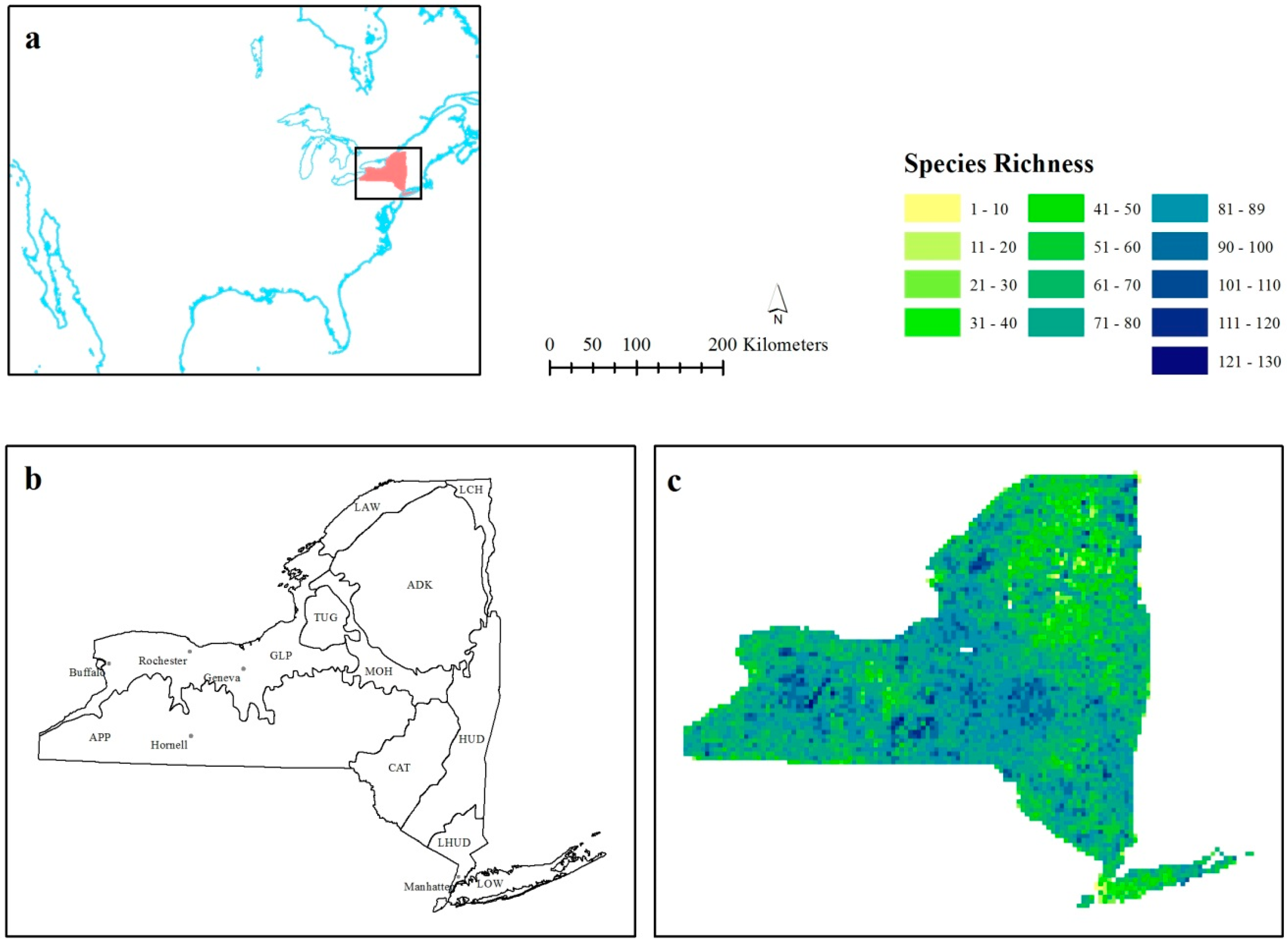
Here we focus on bird species richness data using the New York Breeding Bird Atlas (BBA), which was collected by over 1200 volunteer contributors over a five-year period [39]. The purpose of this research is to investigate how changing the scale of local spatial statistics can be used to explore the environmental factors influencing the bird species richness patterns of New York State. This was done using separate autocorrelation and nonstationarity statistics. Firstly, we use autocorrelation statistics to explore species richness hot- and cold-spots. Secondly, we consider a change in the species richness-environment relationship across the study area as evidenced by a considerable change in the coefficient value to suggest scale-dependent nonstationarity.

2. Material and Methods

2.1. Species Richness and Environmental Data

The BBA surveys cover the entire state in 5 km × 5 km survey blocks and contain three levels of sighting; possible, probable and confirmed, and absences are recorded only if a set of strict protocols were adhered to [40]. The atlas data collected from 2000 to 2005 was used in this study [41], with only confirmed sightings used to generate species richness (Figure 1c). New York State is comprised of eleven ecozones varying in spatial extent (Figure 1b), and has an approximate width and length of 450 km and 500 km respectively.

Figure 1. (a) New York State in relation to North America; (b) the study area with the eleven major ecozones. Ecozones include, the Adirondacks (ADK), Appalachian Plateau (APP), Catskills (CAT), Coastal Lowlands (LOW), Great Lake Plains, (GLP), Hudson Valley (HUD), Lake Champlain (LCH), Lower Hudson Valley (LHUD), Mohawk Valley (MOH), St. Lawrence (LAW), and Tug Hill (TUG); and (c) the species richness data used in the analysis.

Figure 1. (a) New York State in relation to North America; (b) the study area with the eleven major ecozones. Ecozones include, the Adirondacks (ADK), Appalachian Plateau (APP), Catskills (CAT), Coastal Lowlands (LOW), Great Lake Plains, (GLP), Hudson Valley (HUD), Lake Champlain (LCH), Lower Hudson Valley (LHUD), Mohawk Valley (MOH), St. Lawrence (LAW), and Tug Hill (TUG); and (c) the species richness data used in the analysis.

Precipitation and average minimum temperature were obtained from the Parameter-elevation Regressions on Independent Slope Models (PRISM), elevation in the form of a digital elevation model (DEM) was obtained from the USGS, and Enhanced Vegetation Index (EVI) was acquired from the Moderate Imaging Spectroradiometer (MODIS) MOD13 product [42] (see Table 1). EVI was used instead of the more commonly used proxy for vegetation productivity, NDVI, because it is more responsive to canopy structure variations, which strongly influence bird assemblages [43]. Monthly data were averaged for all variables (except elevation) from 2000 to 2005. Data were resampled from their native resolution (see Table 1) using a bilinear technique to 5 km resolution to match the BBA resolution. Prior to analysis, six grid cells, which had zero species richness, were removed. These grids were located over extensive bodies of water (i.e., Peconic Bay and Oneida Lake), and as such were removed from analysis due to lack of land preventing birds from breeding there. Any BBA grid cell with less than 50% of EVI values was deemed to contain more water than land and were subsequently removed from analysis (original n = 5332, final n = 5226). All analysis was undertaken in ArcMap 10.1 [44].

Table 1. Source and resolution of data used in research.

Dataset	Source	Resolution (km)
Breeding Bird Atlas 2005 (BBA)	New York State Breeding Bird Atlas 2000 [41]. Available from: http://www.dec.ny.gov/animals/7312.html	5
Precipitation	PRISM Climate Group, Oregon State University, http://prism.oregonstate.edu/, created 28 September 2011.	4
Minimum Temperature	PRISM Climate Group, Oregon State University, http://prism.oregonstate.edu/, created 28 September 2011.	4
Elevation	National Elevation Dataset: http://ned.usgs.gov/	0.03
Enhanced Vegetation Index (EVI)	MODIS Product 13: Vegetation Indices [42]	1

Table 1. Source and resolution of data used in research.

Dataset	Source	Resolution (km)
Breeding Bird Atlas 2005 (BBA)	New York State Breeding Bird Atlas 2000 [41]. Available from: http://www.dec.ny.gov/animals/7312.html	5
Precipitation	PRISM Climate Group, Oregon State University, http://prism.oregonstate.edu/, created 28 September 2011.	4
Minimum Temperature	PRISM Climate Group, Oregon State University, http://prism.oregonstate.edu/, created 28 September 2011.	4
Elevation	National Elevation Dataset: http://ned.usgs.gov/	0.03
Enhanced Vegetation Index (EVI)	MODIS Product 13: Vegetation Indices [42]	1

2.2. Spatial Nonstationarity—Regression Analysis

Exploration of data identified that relationships between species richness and environmental variables were linear (in line with Austin’s [36] suggestion). Ordinary least squares (OLS) and GWR were subsequently used to examine the relationships between bird species richness and environmental factors. The GWR version of the OLS regression model can be defined as:

$$y_i\left(u\right)= {\beta }_{0i}\left(u\right)+ {\beta }_{1i}\left(u\right)x_{1i}+ {\beta }_{2i}\left(u\right)x_{2i}+\cdots + {\beta }_{mi}\left(u\right)x_{mi}$$

(1)

where y is the dependent variable, there is a set of m independent variable(s), x_k, with k = 1, …, m, and β_0i(u) represents the relationship around location u and is specific to that location. A geographically weighted variance-covariance matrix was used to define the kernel, or neighborhood, within which observations were used. The influence of neighbors was calculated as inversely related to distance through a Gaussian weighting scheme. The bandwidth is a Gaussian measurement of distance, which is in the same units as the coordinate system, and as the bandwidth gets larger, the weights approach unity and the local GWR model approaches the global OLS model.

The choice of an appropriate kernel bandwidth is very important. A bandwidth that is too small will produce an overly local model and an overly large bandwidth will produce results approaching those of a global model. As a result of preliminary exploration of a range of bandwidths (30 km or 6 cells to 450 km or 90 cells), we determined that 120 km was the distance at which these relationships became stationary (where model parameters no longer changed with increasing bandwidth), so we focused on the following four bandwidths: 30 km, 60 km, 90 km, and 120 km.

2.3. Species Richness—Hot-Spot and Cold-Spot Analysis

The G_i* statistic was used to identify spatial clusters of high or low species richness. A positive z-score indicates that the values for most of its neighbors (calculated within the distance variable) are also high, indicating that it is part of a hot-spot, whereas a negative z-score indicates that the neighbors are also low, and identifies a cold-spot [28]. The distance can be changed, altering the neighborhood size, and therefore hot- and cold-spots can be investigated as a function of scale. Distance thresholds matching those used in the GWR analysis were used to explore how richness measurement was scale dependent. The G_i*(d) statistic is defined by:

$$G_i^{*}\left(d\right)=\frac{{{\displaystyle \sum }}_{j=1}^n{w}_{ij}\left(d\right)x_j}{{{\displaystyle \sum }}_{j=1}^n{x}_j}$$

(2)

where w_ij are the elements of the weights matrix, i is a particular location, and d is the radius around i used to define the neighbors, and n is the number of locations.

It should be noted that the neighborhood definitions for GWR and G_i* are not directly comparable. GWR used an inverse-distance weighting function, while G_i* applied equal weighting to all neighbors. However, they can be considered as complementary in terms of studying the effects of scale on spatial pattern. There will also subsequently be inevitable edge effects along the boundary of New York State, as terrestrial state boundaries are not necessarily the end of the extent, and while data limitations prevented us from including observations beyond these boundaries, this is something that should be noted.

3. Results

All four standardized variables were significant in the final OLS model (Table 2). Precipitation and elevation had a negative relationship with bird species richness, possibly due to the inverse physiological tolerances associated with higher rainfall near the coast, and lower temperatures at higher altitudes, while EVI and minimum temperature had a positive relationship, with the benefits of more vegetation for nesting and importance of warmer conditions on the survival of many birds the reason behind these relationships. The variable that had the most influence in the final model was EVI.

Table 2 also shows the descriptive statistics for the final GWR models at the four scales tested here. Precipitation, which had a negative relationship with species richness at the global scale, had a mean positive relationship for all four bandwidths. Similarly, temperature had a negative mean relationship at the smaller bandwidths, despite the positive global relationship. All four environmental variables had a coefficient range whereby the minimum value was negative and the maximum value was positive (Table 2). Elevation was the most important variable at all four bandwidths explored in the GWR analysis, but it was third in importance in the OLS final model.

Table 2. Regression results from ordinary least squares (OLS) and geographically weighted regression (GWR) (tested at four bandwidths). * significant at 0.05, ** significant at 0.01.

OLS		GWR
Explanatory Variables	Coefficients	30 km bw	60 km bw	90 km bw	120 km bw
		Mean (SD)	Mean (SD)	Mean (SD)	Mean (SD)
Intercept	72.32 **	74.6 (14.7)	74.9 (7.5)	75.2 (6.2)	75.3 (5.9)
Precipitation	−0.52 *	1.7 (7.5)	0.9 (4.1)	0.9 (3.5)	1.0 (3.4)
EVI	3.76 **	0.7 (2.2)	1.6 (1.4)	1.7 (1.3)	1.7 (1.3)
Temperature	2.05 **	−1.6 (9.2)	−0.1 (5.3)	0.3 (5.0)	0.5 (5.0)
Elevation	−1.21 **	−3.9 (9.1)	−2.9 (4.8)	−2.7 (4.0)	0.1 (0.1)
R2	0.06	0.143	0.134	0.136	0.137

Table 2. Regression results from ordinary least squares (OLS) and geographically weighted regression (GWR) (tested at four bandwidths). * significant at 0.05, ** significant at 0.01.

OLS		GWR
Explanatory Variables	Coefficients	30 km bw	60 km bw	90 km bw	120 km bw
		Mean (SD)	Mean (SD)	Mean (SD)	Mean (SD)
Intercept	72.32 **	74.6 (14.7)	74.9 (7.5)	75.2 (6.2)	75.3 (5.9)
Precipitation	−0.52 *	1.7 (7.5)	0.9 (4.1)	0.9 (3.5)	1.0 (3.4)
EVI	3.76 **	0.7 (2.2)	1.6 (1.4)	1.7 (1.3)	1.7 (1.3)
Temperature	2.05 **	−1.6 (9.2)	−0.1 (5.3)	0.3 (5.0)	0.5 (5.0)
Elevation	−1.21 **	−3.9 (9.1)	−2.9 (4.8)	−2.7 (4.0)	0.1 (0.1)
R2	0.06	0.143	0.134	0.136	0.137

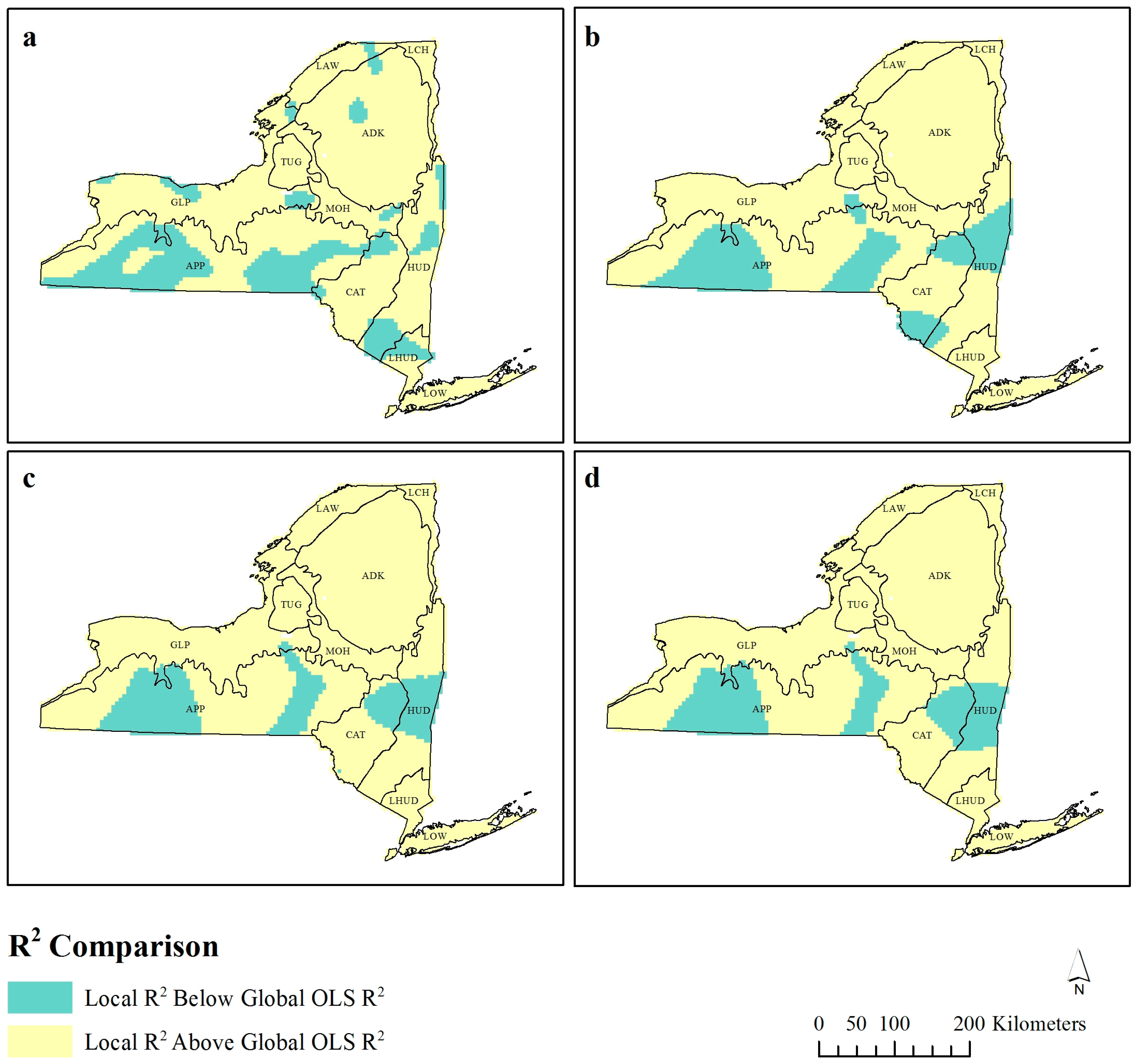
Figure 2. Local R² values for each observation compared to the global ordinary least squares (OLS) R² at bandwidths (a) 30 km, (b) 60 km, (c) 90 km, and (d) 120 km.

Figure 2. Local R² values for each observation compared to the global ordinary least squares (OLS) R² at bandwidths (a) 30 km, (b) 60 km, (c) 90 km, and (d) 120 km.

The mean adjusted R² value was higher at all four bandwidths when compared to the OLS model (Table 2), however, the minimum value of local R² shows that some observations had a lower R² than the global OLS statistic. While this is unsurprising (the global OLS model is effectively a GWR where all locations have equal weight), GWR studies often focus on solely the local R² values that are higher than the global OLS model and little consideration is given to the spatial distribution of these values. At 30 km bandwidth (Figure 2a), there are 12 spatially contiguous “clusters” of lower R² values, and as the bandwidth increases to 90 km (Figure 2c), these decrease in frequency and their extent. At 90 km, the majority of lower R² observations appear consistent in their geographic location.

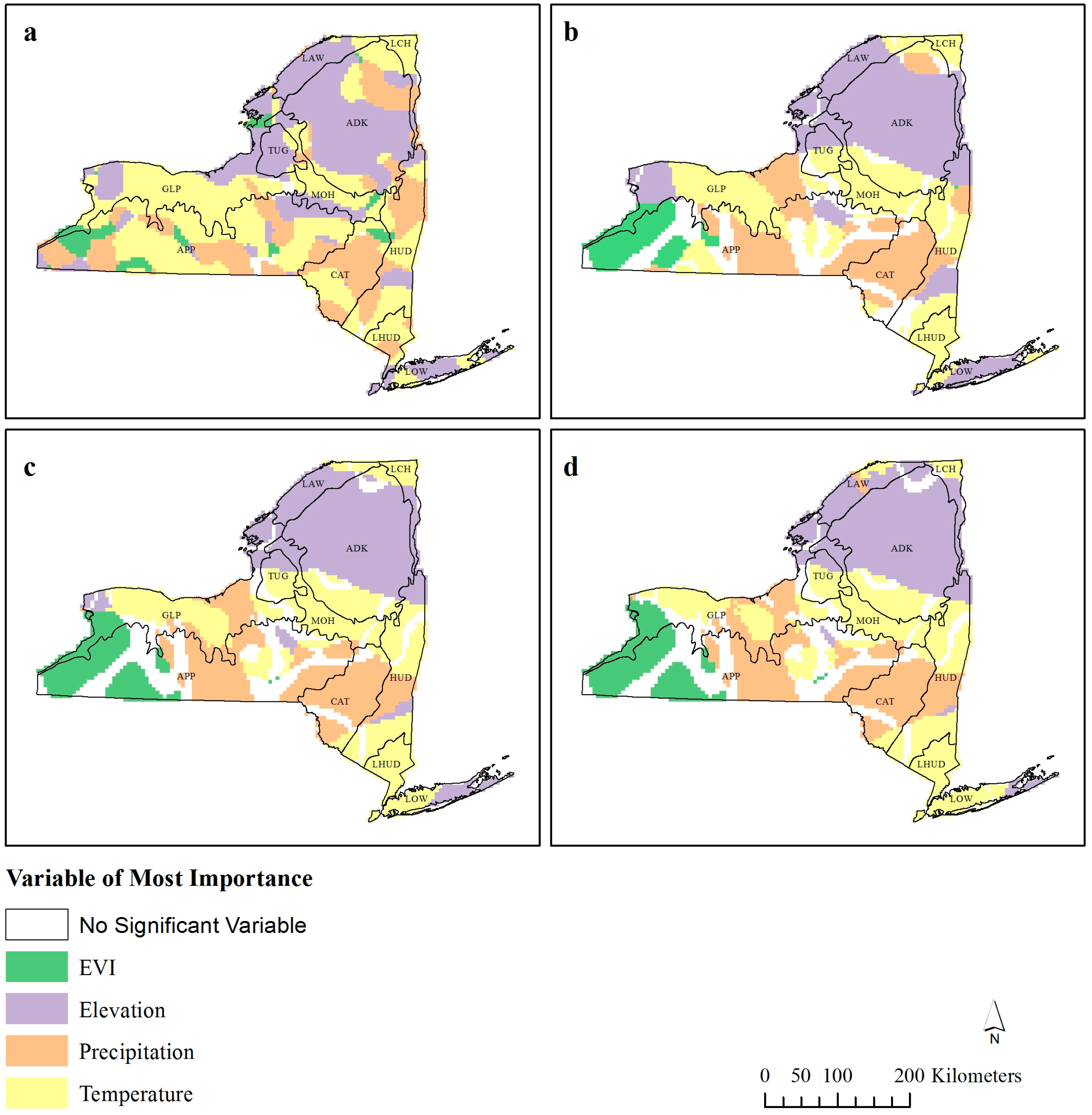
Figure 3. Standardized variable of most importance for geographically weighted regression (GWR) bandwidths (a) 30 km,(b) 60 km, (c) 90 km, and (d) 120 km. Only variables with β > ±1.96 are reported.

Figure 3. Standardized variable of most importance for geographically weighted regression (GWR) bandwidths (a) 30 km,(b) 60 km, (c) 90 km, and (d) 120 km. Only variables with β > ±1.96 are reported.

This spatial exploration of the R² values is important when Figure 2 is compared with Figure 3 and Figure 4, as patterns begin to emerge. The areas of lower local R² values (Figure 2) are situated alongside changes in the significant (β > ±1.96) standardized coefficient of dominance (Figure 3). The humped region of lower R² values which is reported at all four bandwidths in the west of the state and ecozone APP (Figure 2) is located along the border to where EVI and temperature are the dominant coefficients (Figure 3). Likewise, the clumped areas of lower R² values in the east of the state (Figure 2) correspond to the border where precipitation or temperature are considered most important (Figure 3b–d).

Similarly, the humped region of lower local R² values (Figure 2) matches the humped region in Figure 4c, which shows the coefficient inversions of temperature. The strips of positive coefficients changing to negative coefficients as the bandwidth increases appear to follow valley bottoms (DEM: data not shown). As the bandwidth increases, the next valley across inverts its relationship with temperature and richness, most likely a result of the increasing neighborhood capturing richness variations between the productive valley bottoms and the less productive ridgelines. In fact, there appear to be inversions for all independent variables (Figure 4) in all three areas of lower R² values (Figure 2).

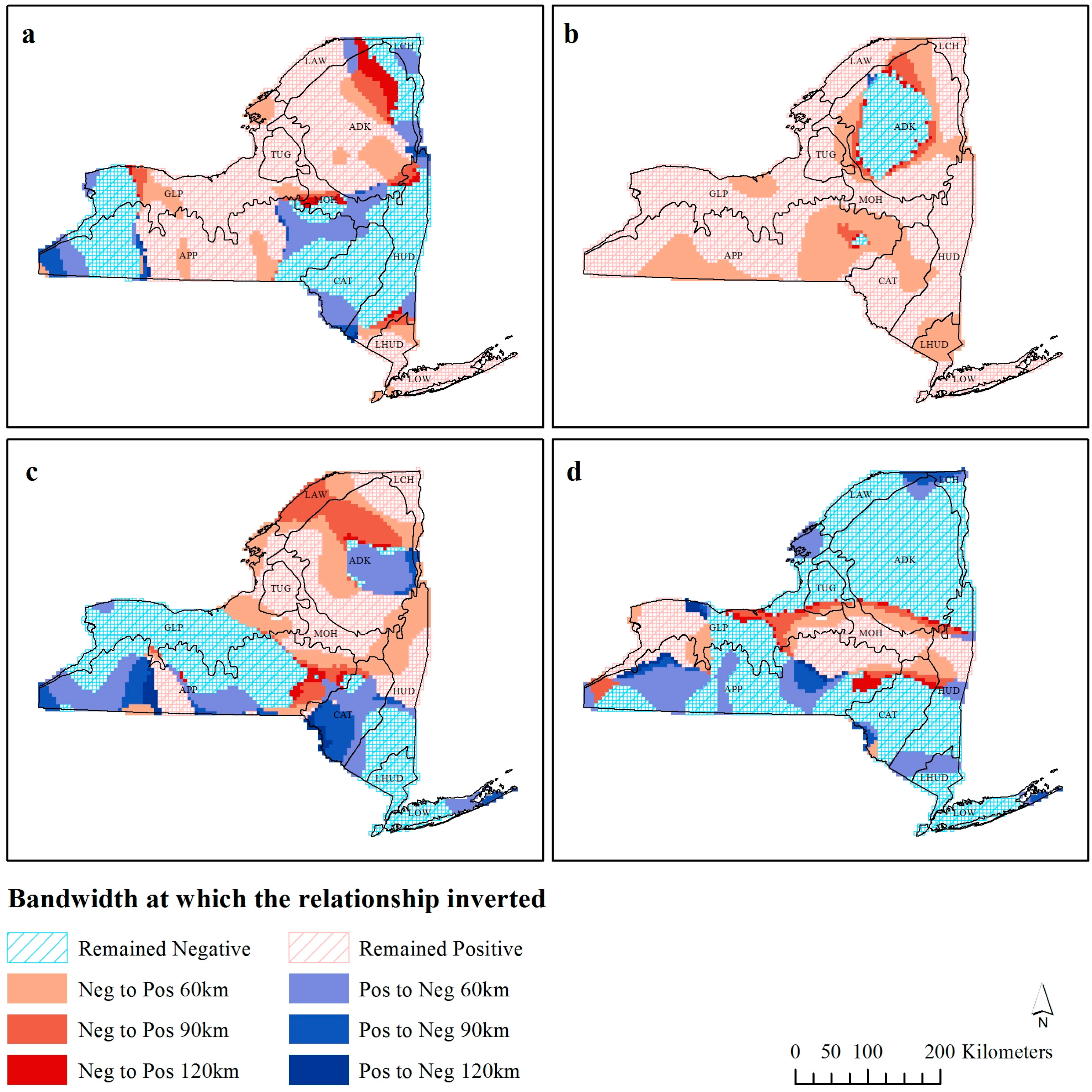
Figure 4. Observations that invert their 30 km richness-environment relationships with increasing scale for (a) precipitation, (b) Enhanced Vegetation Index (EVI), (c) temperature, and (d) elevation.

Figure 4. Observations that invert their 30 km richness-environment relationships with increasing scale for (a) precipitation, (b) Enhanced Vegetation Index (EVI), (c) temperature, and (d) elevation.

Figure 4 shows the bandwidth distance at which coefficients invert their fundamental relationship with species richness (i.e., from positive to negative or vice versa). Precipitation has three distinct regions of positive and negative relationships, with each of these areas expanding as the bandwidth increases. In the northeastern part of the State, the area of negative precipitation richness relationship is constricting, and the three darker bands of red can be observed to illustrate this. Temperature appears to have various relationships at different bandwidths, although in comparison to the other variables, there are fewer observations, which do not invert their fundamental relationship with species richness. In particular, there is a humped shape in the southwest of the state in the Appalachian Plateau (ecozone APP), where at 30 km the whole area has positive observations, and as the bandwidth increases, one half of this area changes to a negative relationship. At 120 km the majority of the study area has a positive richness-EVI relationship, except for the area in ecozone ADK. The areas surrounding the region of negative EVI relationships at 120 km were negative at lower bandwidths, and subsequently as the bandwidth increases, the area of negative relationship would become positive (like the global OLS coefficient). Elevation has a predominantly negative relationship across the state, except for the swath in the middle, which has a positive relationship. Many of the negative observations do not invert, with large extents of continuous observations that do not switch at any distance. There are a handful of observations on the edge of the positive region, which switch from negative to positive as the bandwidth increases, and some in the southwestern part of the state.

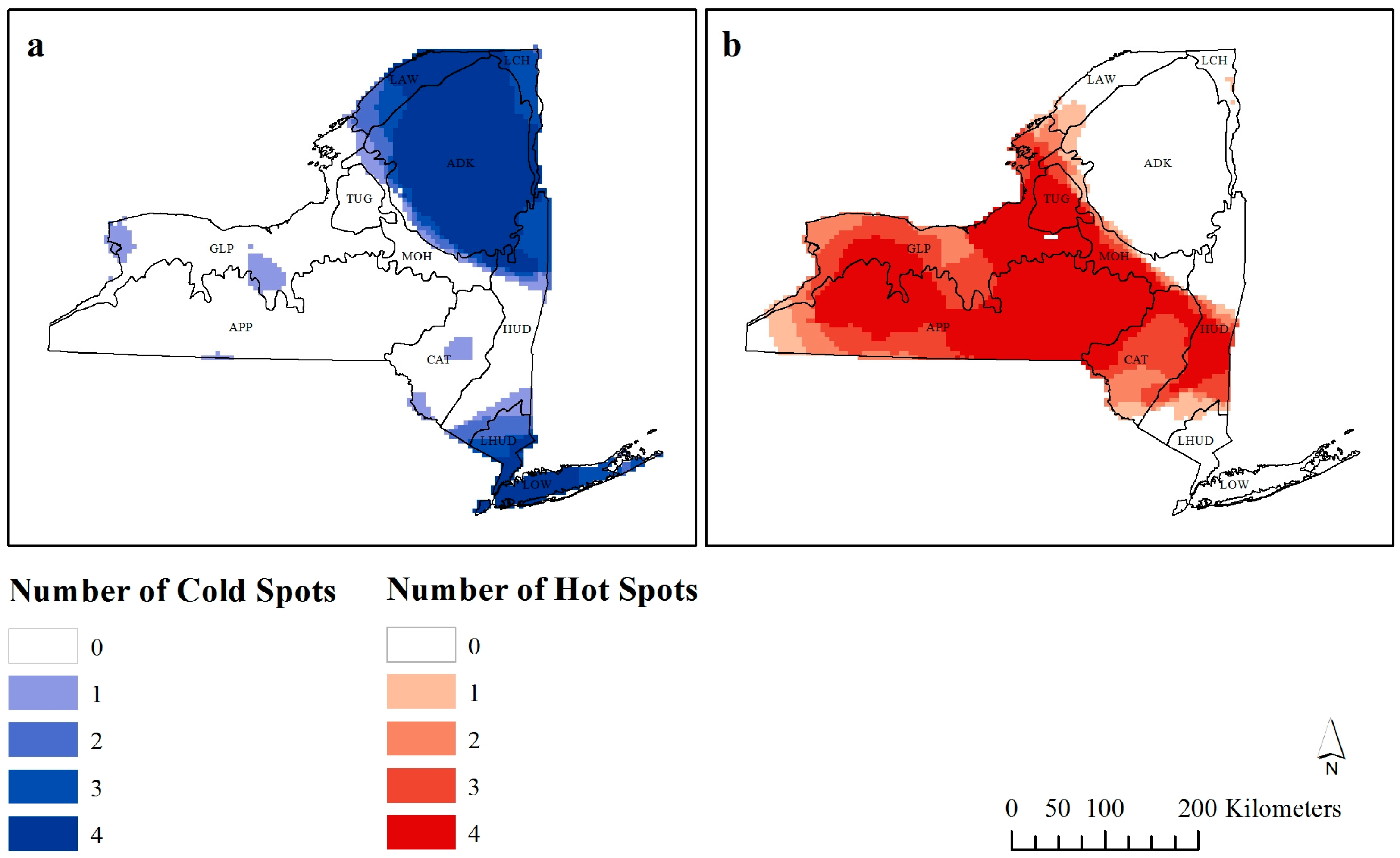
Figure 5. Number of times each observation is considered a (a) cold-spot or (b) hot-spot by Getis-Ord G_i* analysis.

Figure 5. Number of times each observation is considered a (a) cold-spot or (b) hot-spot by Getis-Ord G_i* analysis.

From the 5226 observations, as the distance threshold of the G_i* statistic was increased to 120 km, 3173 observations were considered hot-spots, and 2053 were considered cold-spots. Figure 5 shows how many times each observation is considered a significant hot- or cold-spot (z-score > ±1.96) at different bandwidths. The darker colors are considered scale independent hot- or cold-spots as they are classified as such at a higher number of bandwidths.

4. Discussion

A consistent result of GWR comparison studies is the increased GWR local R² compared to OLS global R² [15,16,18,45]. For example, Foody [15] found that over 90% of the variation between sub-Saharan African bird species richness and a set of environmental variables (climate and NDVI) was explained at fine scales (1°), and that the explained variance decreased as the bandwidth used in the GWR increased (to 8°). It can be observed from Table 2 that the mean local R² value at all bandwidths is higher than the global OLS R², supporting these previous findings.

Local R² values produced with GWR are generally higher than the global R² for reasons related more to local model-fitting than a genuine increase in the explained variance [34,46]. While the local R² may not be the most robust statistic computed by GWR to investigate nonstationarity, there are still observations that have a lower local R² than the global OLS R² value and Figure 2 identifies where these observations are located across New York State, with the spatial pattern of these observations becoming homogenous at 90 km.

The similarity in the areas which exhibit a lower local R² value than the global OLS value (Figure 2) and the areas which showed inversions in the richness-environmental relationship (Figure 4) suggests that areas with a lower local R² value are perhaps subject to the most nonstationarity in the richness-environment relationship, and that the final models are perhaps explaining variance due to some other factor not accounted for in our models. Therefore, any richness-environment relationship observed in these areas should be treated with caution, due to the nonstationarity of the relationship and the low R² observations. However, this does not assume that locations with a greater local R² than the global OLS R² exhibited stationarity, as several nonstationary relationships were observed in these locations, most notably temperature and precipitation (Figure 4a,c).

Ecozone ADK, which contains Adirondack Park (the largest state-level protected area in the contiguous USA), exhibited a scale independent relationship with EVI (Figure 4). While the inverse relationship between EVI and bird species richness may be surprising, this relationship is not uncommon. While Adirondack Park has stable populations of birds, many of these will be forest specific species, and so the species richness will not be particularly high. Fragmentation of surrounding areas may reduce the abundance of a particular species due to loss of habitat, but it creates numerous habitats within the area allowing birds which are not usually associated with this habitat to be found around the edges [47], thus increasing species richness. Therefore, an increase in EVI for fragmented landscapes increases richness, but in a continuous forest landscape it does not. This method of visualizing the results places the richness-EVI relationship in geographic context and makes the interpretation more meaningful.

The stationarity in richness-environment relationship that the coastal lowlands ecozone (LOW) exhibited in all four richness-environment relationships (Figure 4) could be attributed to the uniqueness of this area. Its lower elevation and close proximity to water will both influence the results observed here, as these conditions are not seen throughout the rest of the state and will result in species richness patterns not seen elsewhere. We removed observations that had over 50% water in an attempt to negate some of these impacts, and also to remove any bias that may be observed through a species-area effect (see [48] for a discussion on the species-area relationship). Marine birds were included in the species richness calculations, and while the differences between marine and terrestrial birds may result in different environmental relationships, differentiating among different types of bird species would have resulted in an unmanageable amount of results, and the precautions of removing observations was considered to be sufficient to reduce any possible bias introduced by different physiological traits in the birds. The extensiveness of Manhattan and other urban centers may also have an overwhelming negative impact on richness in the area. There are subsequently a number of scale independent processes occurring in ecozone LOW.

It was unsurprising to find that the area around New York City was consistently a cold-spot when the impact of Manhattan, as well as the specific coastal environmental influences further up the Island are considered. There is also a cold-spot in the northeast of the state, which is where Adirondack Park is found, with reasons for this lower richness already discussed. The true positive richness areas included the area between Buffalo, Rochester and Hornell (locations provided in Figure 1b), as well as the region across the center of the state.

Of note should be the six areas that are both hot- and cold-spots at some bandwidths (Figure 5). Five of these are found within the greater hot-spot cluster, suggesting that these are areas of local scale cold-spots (or low richness). These areas include Buffalo and Geneva (and their surrounding areas). While there has been a recent shift towards increased bird species richness in urban areas due to human provided food sources, especially during winter [49], New York does not appear to follow this trend. While there is no obvious reasoning behind these localized cold-spots, this method of visualization points to areas that require further research as to why these are areas of low richness at local scales but at broader scales are considered hot-spots.

Studies that have investigated changes in G_i* results have generally found an increase in hot-spots at broader scales, irrespective of the phenomena [31,32], although intermediate scales have been found to result in the optimal number of hot-spots (see [33]). Our results do agree with this, and therefore, as the scale of research increases, the data are more likely to become clustered as hot-spots. It should be noted that Nelson and Boots [32] and de Castro et al. [31] studied hot- and cold-spot detection on the magnitude of mountain pine beetle infestations and malaria infestation rates respectively, while Laffan [33] studied weed densities. Our study used species richness, and is subsequently not directly comparable to these other studies. Therefore, more research into how scale influences hot- and cold-spot detection of species richness needs to be undertaken if this spatial analysis is to be used in ecological applications.

Whittaker [50] described a number of ways in which species diversity could be considered. Alpha diversity refers to the total number of species within a habitat, and was considered in our study through the use of species richness. Beta diversity, the differentiation of species between two distinct habitats, as well as gamma diversity, the combination of alpha and beta diversity, could also have been used. While species richness is extremely useful for identifying how biodiverse a region is, it cannot be used to determine if a collection of adjacent observations with high richness contain the same assemblages of species, or completely different ones. Future work should be directed to investigating the impact of scale and local spatial statistics for measures of beta and gamma diversity.

5. Conclusions

Identification of species richness and environmental relationships, and the inclusion of methods to identify and analyze spatial autocorrelation and nonstationarity are critical elements for conservation. The use of localized spatial statistics can provide a direct way of assessing and visualizing the richness-environment relationships. While studies have looked at how changes in scale influence the results obtained from local spatial statistics, it is still a relatively understudied area of research, and by systematically altering neighborhood sizes, it is possible to identify how persistent these relationships are across multiple scales. We found that there were considerable local differences in relationships between EVI, precipitation, elevation, temperature and bird species richness at different definitions of neighborhoods, which has important implications for any management strategies applied on the results of such analysis. Where these changes occur, and at what bandwidth, are important aspects of exploratory analysis, and while previous studies (e.g., [15]) have “tracked” the species-environment relationships for individual observations as the scale of the local spatial statistics is systematically changed, by developing a new visualization technique to map these scale changes in local spatial statistics, the location of nonstationarity and autocorrelation can be interpreted in geographic context, across the entire study area. The inversions in richness-environment relationship with scale (e.g., from positive to negative) can have serious implications on any management strategies based on analysis, and so researchers need to study these patterns at a variety of scales. This visualization technique allowed us to identify patterns which began to emerge between nonstationarity, local R² values and variables of most importance. The use of localized spatial statistics allows for more detailed environmental analysis, and offers a chance to explore species richness patterns at varying spatial scales in a variety of visualizations.