Article

Land Cover Heterogeneity Effects on Sub-Pixel and Per-Pixel Classifications

1
Department of Geography and Environmental Sustainability, University of Oklahoma, Norman, OK 73019, USA
2
Department of Geography, Texas State University, San Marcos, TX 78666, USA
*
Author to whom correspondence should be addressed.
ISPRS Int. J. Geo-Inf. 2014, 3(2), 540-553; https://doi.org/10.3390/ijgi3020540
Submission received: 1 January 2014 / Revised: 3 March 2014 / Accepted: 17 March 2014 / Published: 3 April 2014

Abstract

:
Per-pixel and sub-pixel are two common classification methods in land cover studies. The characteristics of a landscape, particularly the land cover itself, can affect the accuracies of both methods. The objectives of this study were to: (1) compare the performance of sub-pixel vs. per-pixel classification methods for a broad heterogeneous region; and (2) analyze the impact of land cover heterogeneity (i.e., the number of land cover classes per pixel) on both classification methods. The results demonstrated that the accuracy of both per-pixel and sub-pixel classification methods were generally reduced by increasing land cover heterogeneity. Urban areas, for example, were found to have the lowest accuracy for the per-pixel method, because they had the highest heterogeneity. Conversely, rural areas dominated by cropland and grassland had low heterogeneity and high accuracy. When a sub-pixel method was used, the producer’s accuracy for artificial surfaces was increased by more than 20%. For all other land cover classes, sub-pixel and per-pixel classification methods performed similarly. Thus, the sub-pixel classification was only advantageous for heterogeneous urban landscapes. Both creators and users of land cover datasets should be aware of the inherent landscape heterogeneity and its potential effect on map accuracy.

Graphical Abstract

1. Introduction

Land cover maps derived from remotely sensed images are widely used to investigate human-environment interactions [1]. Accordingly, concern about the accuracy of these maps has grown. If accuracy refers to “the degree of “correctness” of a map” [2], accuracy assessment is a process of quantifying the degree to which the derived map conforms to the ground “truth” [2]. The confusion matrix is a key means for accuracy assessment, because it quantifies not only the overall accuracy, but also the errors of omission and commission associated with individual map classes [2,3]. However, the confusion matrix is set by the resolution of the imagery and, thus, assumes that each pixel is homogenous. In areas with small land cover features (e.g., isolated trees) or high land cover heterogeneity (e.g., urban areas), the confusion matrix may not characterize the full extent of land cover accuracy [4]. Since the last decade, there has been a call to move beyond the confusion matrix to include the spatial pattern of classification errors when documenting the accuracy of land cover maps [4,5,6]. Understanding the spatial variation of these errors helps scientists to identify whether regions of interest have sufficient accuracy [4] or to pin point regions of low accuracy for further classification enhancement procedures [5,7]. In order to reveal the spatial pattern of these errors, it is necessary to recognize their sources.
In addition to errors associated with sensor limitations and atmospheric effects, landscape characteristics (i.e., the spatial arrangement and properties of land cover) can also be a source of error [8]. Elevation, for example, has been found to both enhance and reduce classification accuracy. In the former case, vegetated regions at higher elevation may have higher classification accuracy, because phenology at higher elevations tends to be more homogeneous [9]. In the latter case, drastic elevation changes can cause variation in brightness values between a horizontal surface and a sloped surface for the same land cover [10].
Patch size and land cover heterogeneity (i.e., the number of land cover types found within a defined spatial window, which can be a pixel, a block of pixels or a study region) can also have an effect on classification accuracy. Typically, larger patches have higher accuracy, while more heterogeneous patches have lower accuracy [11,12]. For example, the probability of a correct classification of a Landsat pixel will be greater than 0.5 if it is contained in a patch of 56 × 56 pixels or if it is homogeneous [13]. Depending on the image resolution and classification method used, the influence of patch size and heterogeneity on accuracy may be different. Heterogeneity can reduce per-pixel classification accuracy by increasing intra-class variation if the image resolution is fine or by increasing the number of mixed pixels (i.e., pixels comprising more than one land cover type) if the image resolution is coarse [14]. The mixed-pixel problem, however, may be resolved by applying sub-pixel classification to unmix the pixels to land cover proportions [15,16,17].
Although sub-pixel classification has potential in a variety of applications [18,19,20], its accuracy is still affected by high intra-class variation caused by land cover heterogeneity [16,21]. While statistical analyses have been performed to examine the effect of land cover heterogeneity on per-pixel classification [11,13,22], the same has not been done for sub-pixel classification. Therefore, the objectives of this study are to: (1) analyze the effects of land cover heterogeneity on sub-pixel classification; and (2) compare sub-pixel classification with per-pixel classification over a broad heterogeneous region to assess in which landscapes sub-pixel classifications may be advantageous.

2. Study Area

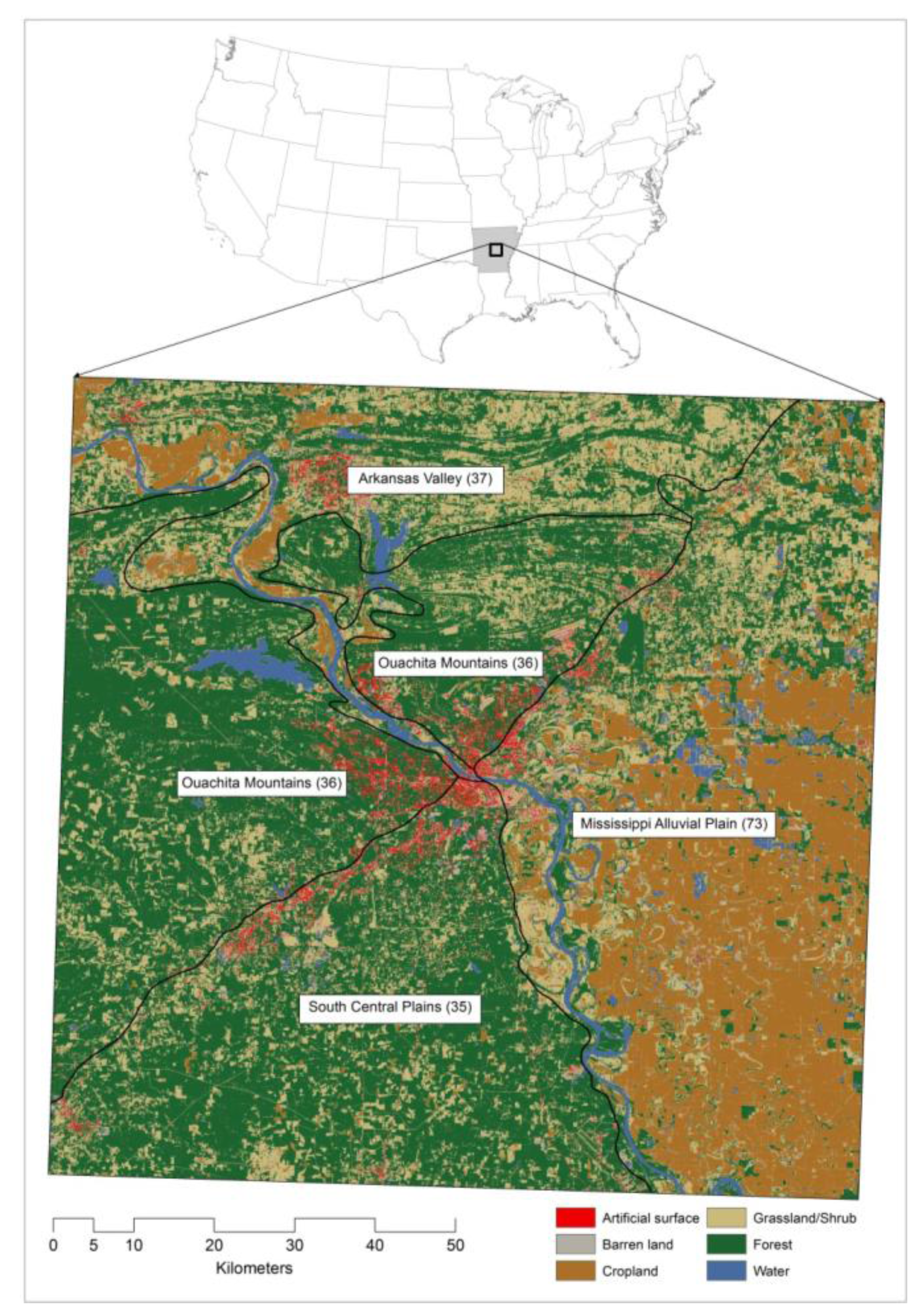
This study examines a 10,000 km2 area in central Arkansas (USA), centered on the capital of Little Rock (Figure 1). This area was selected because of its heterogeneity in physiography and land cover. Little Rock is situated at the intersection of four Omernik Level III ecoregions [23]. The Arkansas Valley ecoregion north of Little Rock is characterized by forested hills (31% forest in 2006) that bound large valleys covered in a mixture of agricultural activities (9% cropland). The Mississippi Alluvial Plain to the east is a relatively flat ecoregion historically covered by forested wetlands and several large grasslands, but is now agriculturally dominated (54% cropland). South of Little Rock lays the South Central Plains ecoregion, composed of rolling forested plains (54% forest) with many small patches of urban (14%), agriculture (0.4%) and barren (0.3%) lands. The Ouachita Mountains ecoregion to the west is mostly forested (68%), with steep slopes along east-west trending ridges. Commercial logging is the major land use in these latter two ecoregions. More details of land cover composition within this study area, as well as temporal changes and their drivers can be found in Jawarneh and Julian [24]. In all, land cover is most heterogeneous in the Arkansas Valley, followed by the South Coastal Plains, the Mississippi Alluvial Plain and, lastly, the Ouachita Mountains.
Figure 1. The study area centered on Little Rock, Arkansas, USA. The base layer is the land cover map (2010; 30-meter resolution) generated by the per-pixel classification in this study. The four Omernik Level III ecoregions are outlined in black.
Ijgi 03 00540 g001

3. Data

Landsat imagery (30-m resolution) and aerial photographs (1-m resolution) were used to analyze the impact of land cover heterogeneity on per-pixel and sub-pixel classification methods. Landsat 5 Thematic Mapper (TM) images (Path 24, Row 36) at Level 1T with six bands (excluding the thermal band) were downloaded from the U.S. Geological Survey (USGS) Earth Explorer. To reduce confusion between cropland and other land covers (e.g., barren and grassland/shrub), this study used multi-seasonal images acquired on 12 April 2010, 19 September 2010, and 6 November 2010. These images were cloud-free and closest to the acquisition date of the National Agriculture Imagery Program (NAIP) photos (June–September 2010). Fast Line-of-sight Atmospheric Analysis of Spectral Hypercubes (FLAASH) [25] was used to convert Landsat images from top-of-atmosphere radiance to surface reflectance. Ultimately, all images were layer-stacked and subset to the predefined 100 × 100 km2 study area.
Land cover types were classified by a per-pixel classification using the supervised Maximum Likelihood Classification (MLC; [26]) and by a sub-pixel classification using the supervised Fuzzy Maximum Likelihood Classification (FMLC; [27]). Training and validation data for these classification methods were developed based on the National Land Cover Database 2006 (NLCD 2006; [28]) and NAIP aerial photos obtained from the U.S. Department of Agriculture (USDA) Geospatial Data Gateway [29]. These 1-m resolution natural-color photos were acquired during the agricultural growing seasons and were administered by the USDA Farm Service Agency through the Aerial Photography Field Office in Salt Lake City. NAIP photos were available as orthorectified photos with a reported horizontal accuracy of 6 m [29,30].

4. Methodology

4.1. Classification

The land cover classes in Table 1 were used for both per-pixel and sub-pixel classification methods. The training and validation data were developed using stratified random samples. By aggregating similar NLCD 2006 classes, we identified seven land cover strata: water (NLCD Class 11), artificial surface (21, 22, 23, 24), barren land (31), forest (41, 42, 43), grassland/shrub (52, 71, 81), cropland (82) and wetland (90, 95). We did not incorporate the wetland class in our classification scheme, due to its easy confusion with other land cover classes (e.g., agricultural crops and upland forests) (Table 1) [31], but it was considered in the sampling strategy in order to account for the spectral variation of forest cover in wetland and upland areas. For each sample, its land cover proportions were determined by visually interpreting the 2010 NAIP aerial photos.
Training samples are recommended to be homogeneous (i.e., composed of only one land cover type) to make sure that the radiance histogram of a class is unimodal to facilitate the calculation of statistical measures (e.g., mean and covariance matrix) [32]. However, in a heterogeneous landscape, selecting homogeneous samples can be problematic, because it is difficult to have enough homogeneous samples located in all parts of the study area. Moreover, as the landscape becomes more heterogeneous with mixed pixels, the radiance data extracted from samples may not be representative of other mixed pixels for the same class. That is, pixel radiance is a function of radiance from all classes within the pixel and its neighboring pixels [27]. Accordingly, our samples (“soft” training samples) consisted of anywhere from one to seven land cover types. In all, we used 1575 samples (225 “soft” training samples per land cover class). The size of “soft” training samples was one Landsat pixel (30 × 30 m). Land cover proportions for each training sample were estimated by visually interpreting NAIP photos at a scale of 1:2000. These “soft” training samples were used in sub-pixel classification. For per-pixel classification, however, “hard” training samples were used. These “hard” training samples were created by applying the dominant rule to the “soft” training samples. We used the Maximum Likelihood Classification algorithm (per-pixel) to produce a categorical map with six classes (i.e., wetland classes were converted to the forest class) and the Fuzzy Maximum Likelihood Classification algorithm (sub-pixel) to produce a fractional map constructed by overlaying six proportional images, each of which represented a land cover type. The sum of all land cover proportions within pixels of the fractional map was one, because it was the assumption of the FMLC [27].
Table 1. Land cover classes adapted from the National Land Cover Database 2006 (NLCD 2006).
ClassDefinition
Cropland (CR)Areas used for the production of crops, such as corn, soybeans, vegetables, tobacco and cotton. This class also includes fallow cropland.
Artificial surface (AR)Construction materials, such as asphalt, concrete and rooftops.
Barren (BA)Areas of bedrock, bare soil, quarries and any accumulation of earthen material.
Forest (FO)All trees over 5 m, including low-density trees in urban areas.
Grassland/Shrub (GR)Areas with >80% coverage of graminoid or herbaceous vegetation; or areas with >20% coverage of shrubs less than 5 m high.
Water (WA)Areas of open water with <25% coverage of any other class.

4.2. Validation

In this study, we used the cross tabulation matrix [33] proposed as a customization of the conventional confusion matrix [34] to validate the performance of the two classification methods. The cross tabulation matrix aims at assessing the accuracy of a classification at the sub-pixel scale. Therefore, unlike the conventional confusion matrix measuring the agreement/disagreement between a categorical map resulting from a per-pixel classification and a set of “hard” validation samples, each of which consists of exactly one class, the cross tabulation matrix measures the agreement/disagreement between a fractional map resulting from a sub-pixel classification and a set of “soft” validation samples, each of which consists of more than one class [33]. For a study area, while there is exactly one conventional confusion matrix, there may be multiple cross tabulation matrices, each of which is created for each “soft” validation sample. In a cross tabulation matrix, diagonal entries represent the agreements calculated as the overlapped class proportions between a “soft” validation sample and a corresponding pixel (or block of pixels) in the fractional map. Similarly, off-diagonal entries represent the disagreements calculated based on the non-overlapped class proportions. In addition to the individual cross tabulation matrices created for the “soft” validation samples, an overall cross tabulation matrix can be created for an average validation sample to characterize the accuracy of a classification at the level of the study area. The average validation sample consists of all classes found in all “soft” validation samples. A proportion of each class in the average validation sample is calculated as an average of the proportions of the same class across all “soft” validation samples. Both individual and overall cross tabulation matrices can be used for either sub-pixel or per-pixel classification. In the case of per-pixel classification, “soft” validation samples can be used to validate a categorical map with the assumption that the class proportion of pixels in the categorical map equals 100%.
In this study, individual cross tabulation matrices and overall cross tabulation matrices were created for both per-pixel and sub-pixel classification methods based on 700 “soft” validation samples (100 per sampling class). The size of “soft” validation samples was a block of 3 × 3 pixels to reduce the effect of misregistration between the referenced NAIP photos and the Landsat data [35,36]. For each validation sample, we estimated reference land cover proportions by visually interpreting the NAIP photos at the scale of 1:2000, which was equivalent to the procedure applied to the training samples. Besides, for each classification method, using the individual cross tabulation matrices, we were able to determine the producer’s and user’s accuracies for “soft” validation samples to facilitate the statistical analysis of the impact of heterogeneity on the classification accuracies. Furthermore, the overall cross tabulation matrix provided a general understanding about the misclassifications between classes for each classification method.

4.3. Statistical Analyses

In these statistical analyses, land cover heterogeneity was calculated for each validation sample as the number of land cover types existing within the sample. For instance, a sample occupied by two land cover types has a land cover heterogeneity of two classes. Samples having the same heterogeneity were grouped into six groups, ranging from one to six. Because there were too few (<5) samples in group six, this group was excluded from further statistical analyses.
In order to test the effect of heterogeneity on classification accuracies, two statistical tests were performed based on the “soft” validation samples. First, the Wilcoxon signed-rank test was conducted to test whether differences in the producer’s and user’s accuracies between the two classification methods were significant. Second, the Steel–Dwass test was conducted to study whether a change in the number of land cover classes (i.e., heterogeneity) would result in significant change in the producer’s, user’s and overall accuracies of both classification methods. These two non-parametric tests were conducted because the producer’s and user’s accuracies of the two classification methods were not normally distributed.

5. Results and Discussion

5.1. Land Cover Map and Accuracy
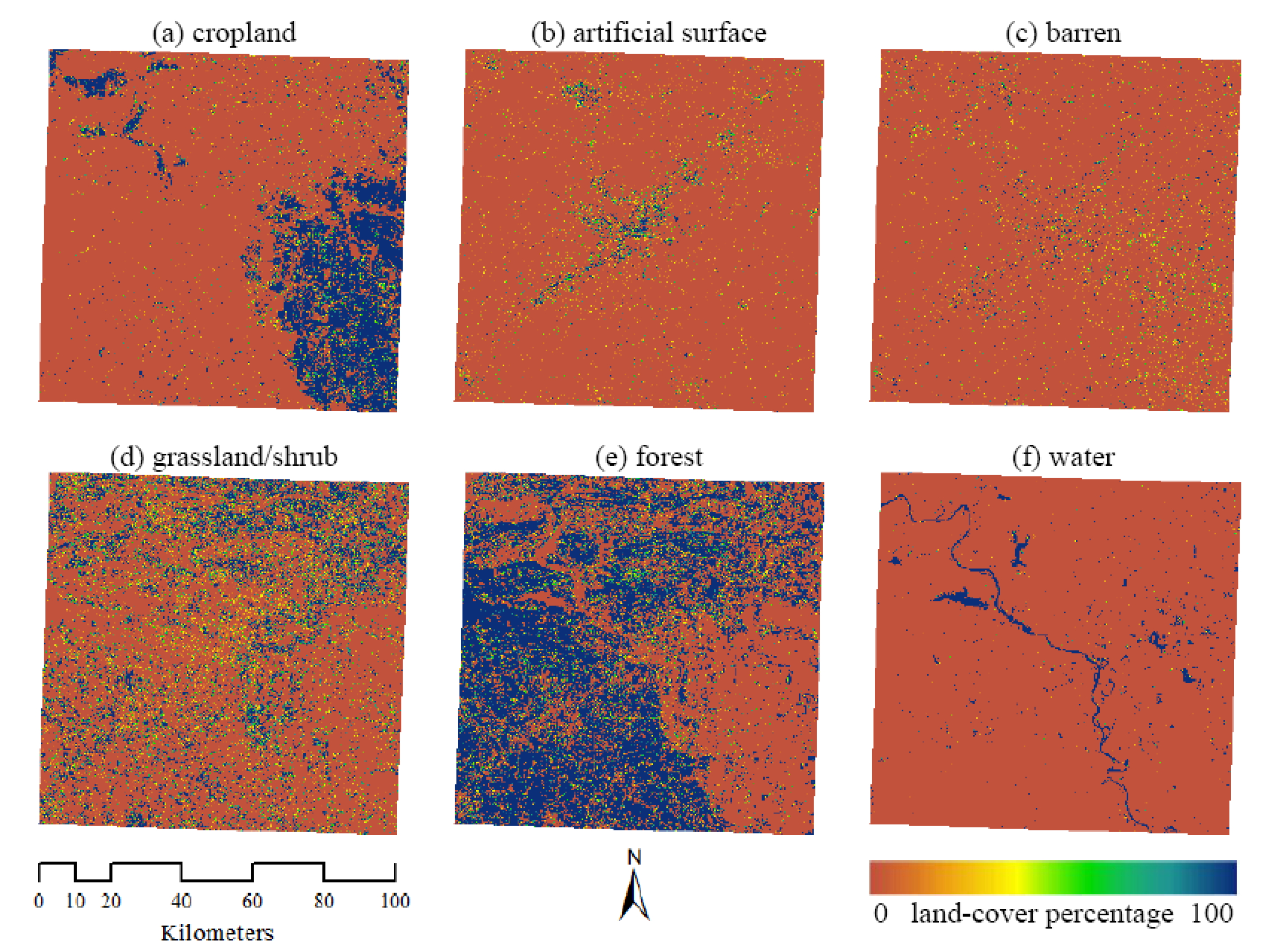
The categorical per-pixel land cover map (Figure 1) and the fractional sub-pixel land cover maps (Figure 2) provide two different perspectives of the same landscape with similar accuracy. The per-pixel classification had an overall accuracy of 81.9%, and the sub-pixel classification had an overall accuracy of 82.3% (Table 2). Although these overall accuracies were slightly lower than the common threshold of 85% [37], they were acceptable, because: (1) they were in a range of the accuracies published during the last decade [38]; (2) they exceeded the level of 75% suggested by Goodchild et al. [39]; and (3) they were higher than the regional accuracy of NLCD 2001, Level I (79% for Region 7; [40]). Indeed, this South-Central U.S. region has the lowest overall accuracy for the NLCD, likely due to high landscape heterogeneity and large areas of ephemeral wetlands [40].
Figure 2. Land cover percentages (2010; 30-m resolution) generated by the sub-pixel classification.
Ijgi 03 00540 g002
Table 2. The overall cross tabulation matrix for the two classification methods: per-pixel (normal text) and sub-pixel (bold italicized text).
Land Cover ClassReferenced Percentage
CroplandArtificialBarrenGrass-Land/ShrubForestWaterTotal
Estimated percentageCropland12.650.050.780.910.440.1815.00
12.400.040.730.880.380.0814.51
Artificial0.014.870.780.620.370.046.68
0.065.871.151.090.510.078.75
Barren0.382.336.011.170.610.3110.81
0.501.805.780.900.580.339.88
Grassland/Shrub1.610.650.3717.931.580.1922.33
1.670.250.2217.561.350.2121.24
Forest0.090.590.252.9429.110.2433.22
0.110.520.293.1329.290.2133.54
Water0.040.000.130.280.2111.3011.95
0.040.010.150.280.2211.3712.07
Total14.788.488.3223.8432.3212.26100.00
14.788.488.3223.8432.3212.26100.00
Overall accuracy (%)81.87 Kappa (%)76.99
82.2877.54
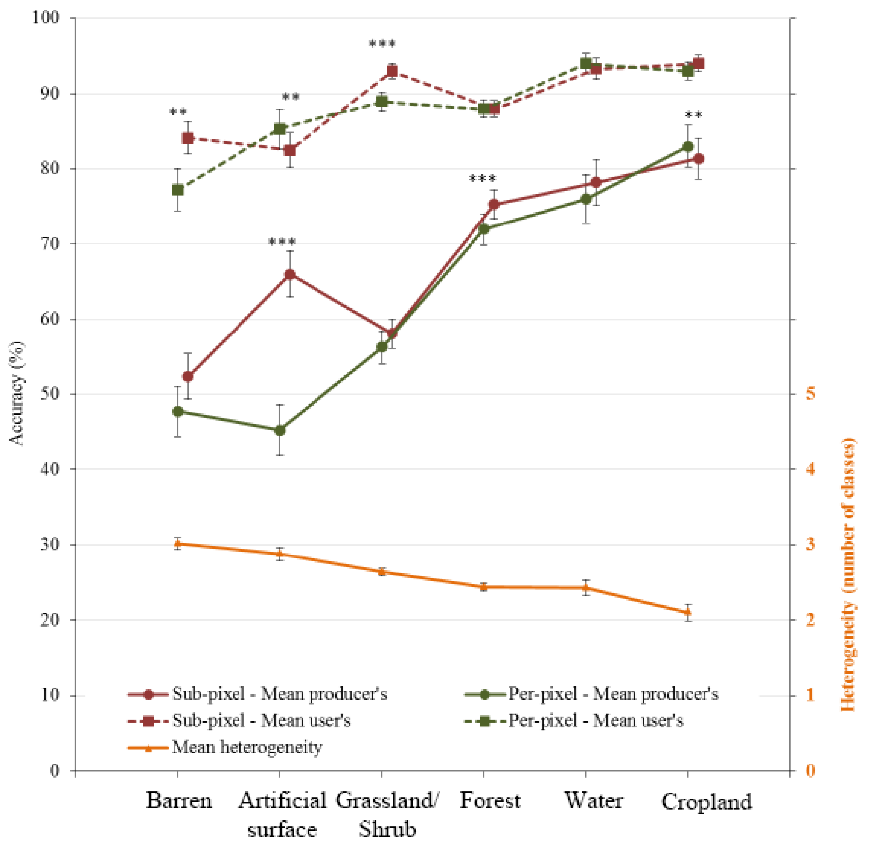
Among all classes, cropland had the highest producer’s and user’s accuracies (Figure 3). Using multi-seasonal Landsat data to identify cropland definitely improved these accuracies, but we argue in the next section that it has more to do with croplands having low heterogeneity. Nevertheless, misclassifications did occur for croplands, particularly between fallow cropland and barren lands (Table 2). Barren and artificial surfaces were also confused. In the per-pixel classification, 27% (2.33/8.48) of artificial surfaces was misclassified as barren and 9% (0.78/8.32) of the barren surface was misclassified as artificial surface. In the sub-pixel classification, 21% (1.8/8.48) of the artificial surface was misclassified as barren and 14% (1.15/8.32) of the barren surface was misclassified as artificial surface.
Figure 3. The mean producer’s and user’s accuracies of per-pixel and sub-pixel classification methods together with the mean number of classes across all 3 × 3 pixels “soft” validation samples. The mean of producer’s and user’s accuracies were calculated as the averages of all producer’s and user’s accuracies taken from the individual cross tabulation matrices developed for all “soft” validation samples. The error bars represent one standard error. The asterisks indicate * p < 0.05, ** p < 0.01 and *** p < 0.001 from the Wilcoxon signed-rank test.
Ijgi 03 00540 g003
An exploration of these classification errors revealed that the misclassifications between the artificial surface and the barren surface occurred due to spectral similarities between high-albedo artificial surfaces (i.e., rooftops) and barren (i.e., sand and dry soil), as well as between low-albedo artificial surfaces (i.e., asphalt and roads) and barren surfaces (i.e., gravel) [41,42,43,44]. Artificial surfaces were also confused with grassland/shrub (nearly 8% for per-pixel and 3% for sub-pixel), as well as forest (7% for per-pixel and 6% for sub-pixel). The most likely reason was the spectral similarity in the near-infrared band between high-albedo artificial surface and vegetation [42]. Barren surfaces were confused with cropland, grassland/shrub and forest, especially along class boundaries, such as narrow and/or linear farm paths, forest paths and dirt shoulders along tree-lined roads. These misclassifications showed that both per-pixel and sub-pixel classification methods had difficulty in identifying narrow/linear features [12]. This difficulty in identifying narrow/linear features might also explain some of the misclassifications between forest and grassland/shrub, which were commonly found in low-intensity residential areas and open woodlands. Spectral confusion was also a likely culprit for some of these misclassifications [45].
Wilcoxon signed-rank tests were conducted to test the differences between the producer’s accuracies of per-pixel vs. sub-pixel classification methods and the differences between the user’s accuracies of per-pixel vs. sub-pixel classification methods for each land cover class (Figure 3). User’s accuracies were similar for all land cover classes, except for barren (p < 0.05) and grassland/shrub surfaces (p < 0.001), which were significantly higher for sub-pixel classification, and artificial surface, which was significantly higher (p < 0.05) for per-pixel classification. The producer’s accuracy of sub-pixel classification was significantly higher than that of per-pixel classification for artificial surface (p < 0.001) and forest (p < 0.001) classes (Figure 3). Most notably, while the difference between the producer’s accuracy of sub-pixel vs. per-pixel classification for most classes was small (<5%), sub-pixel classification performed far better for artificial surfaces with a producer’s accuracy that was 20% higher than for per-pixel classification. This finding was supported by claims that sub-pixel classification is more advantageous than per-pixel classification, because it relaxes the assumption that pixels are homogenous [46,47]. Many studies, especially urban studies characterizing artificial surfaces with remote sensing data, have been successful in using sub-pixel classification to develop fractional maps of land cover types [19,48,49]. For other classes, the preference of sub-pixel vs. per-pixel classification remains a debate, because the producer’s and user’s accuracies were not consistently higher for one classification over the other (Figure 3). However, classifiers other than FMLC (e.g., spectral mixture analysis, fuzzy c-means, neural network) could have provided a different result where sub-pixel classification would have been better than per-pixel classification for classes other than artificial surfaces. A note of caution is that Landsat data, with a resolution of 30 m, likely does not produce many mixed pixels, which may have masked differences between per-pixel and sub-pixel classification methods in our study. For coarser resolution data, such as MODIS, sub-pixel classifications may be needed to properly characterize land cover/use in heterogeneous landscapes.

5.2. Heterogeneity and Its Effect on Classification Accuracy

Both the per-pixel (Figure 1) and sub-pixel (Figure 2) land cover maps show varying levels of heterogeneity across the study area. Cropland-dominant areas tended to have the lowest heterogeneity, while urban areas tended to have the highest heterogeneity. Among the six classes, barren validation samples were most heterogeneous, with an average heterogeneity of 3.0 classes (i.e., any “soft” validation samples containing barren land typically had three classes), followed closely by artificial surfaces at 2.9 (Figure 3). In contrast, cropland validation samples were the least heterogeneous, with an average heterogeneity of 2.1 classes. Given that barren and artificial surface were mostly found in urban areas, while grassland/shrub and cropland were found in rural areas, the trend of decreasing heterogeneity from barren to cropland suggests that the urban landscape is more heterogeneous than the rural landscape.
A rural-urban heterogeneity trend was also evident in the producer’s and user’s accuracies of the per-pixel classification, where urban areas usually had lower accuracy and rural areas had much higher accuracy (Figure 3). In other words, where land cover was less heterogeneous, the accuracies of per-pixel classification were higher. This result was similar to the findings from other scholars for per-pixel classification [11,13,22]. Interestingly, we found that this trend generally held for sub-pixel classification, as well. The exception was artificial surfaces, due to their exceptionally high producer’s accuracy (see the previous section). Overall, the accuracy of per-pixel classification is expected to decrease as pixels become more heterogeneous [11,13]. This is likely the reason why most sub-pixel classifications have been conducted in urban landscapes with large areas of artificial surfaces, e.g., [50,51].
The effect of heterogeneity on classification accuracy was further analyzed by testing the differences in the mean rank of the overall accuracy, as well as the producer’s and user’s accuracies among groups of heterogeneity using the Steel–Dwass non-parametric test. The results demonstrated that the accuracies of validation samples having one class (heterogeneity = 1 class) were significantly and distinctly the highest, followed by validation samples with two classes. If a validation sample had three or more classes, its accuracy dropped considerably, and in general, there were no significant differences among validation samples with a heterogeneity of three, four or five classes. These findings further support our previous results that increasing land cover heterogeneity reduces the accuracy of both per-pixel and sub-pixel land cover classification methods.
While the variation in accuracy among validation samples with three or more classes was not significant, such variation could be due to other factors, such as difference in the spatial extents of classes within validation samples or due to misregistration between NAIP photos and Landsat data. In fact, classes having a small spatial extent often have low accuracy in per-pixel classification [11,12]. The effect of misregistration on the classification accuracy in this study was expected to be small due to the use of window-based (3 × 3 pixels) validation samples. Indeed, other studies indicated that increasing the window size of validation samples could result in increased accuracy [35]. However, this study used the window size of 3 × 3 pixels because if the window size was greater than 3 × 3 pixels, it would be difficult to visually estimate proportions of all land cover types within the samples, due to their high heterogeneity.

6. Conclusion

From our study of a broad heterogeneous landscape, we found that: (1) both per-pixel and sub-pixel classification accuracies are reduced by land cover heterogeneity; and (2) sub-pixel classification performs better overall than per-pixel classification for artificial surfaces. Therefore, when faced with the decision of using a per-pixel or sub-pixel classification, sub-pixel classification may only become advantageous for heterogeneous urban landscapes. For all other types of landscapes, the extra time involved in producing a sub-pixel classification is probably not worth the time spent on developing its “soft” training and “soft” validation samples. Our experience showed that the time needed to visually estimate all land cover proportions within 50 training samples for a sub-pixel classification was 15 times longer than the time needed to visually identify the dominant land cover type within the same 50 training samples for a per-pixel classification. Regardless of which type of classification is used or the intended application, both creators and users of land cover datasets should be aware of the inherent landscape heterogeneity and its potential effect on map accuracy.

Author Contributions

Trung V. Tran conceived and designed the study, performed the research, analyzed the data, and wrote the manuscript. Jason P. Julian helped design the study, assisted with writing, and contributed editorial input. Kirsten M. de Beurs helped design the study and contributed editorial input.

Conflicts of Interest

The authors declare no conflict of interest.

References

  1. Turner, B.L.; Lambin, E.F.; Reenberg, A. The emergence of land change science for global environmental change and sustainability. PNAS 2007, 104, 20666–20671. [Google Scholar] [CrossRef]
  2. Foody, G.M. Status of land cover classification accuracy assessment. Remote Sens. Environ. 2002, 80, 185–201. [Google Scholar] [CrossRef]
  3. Congalton, R.G. Accuracy Assessment of Remotely Sensed Data: Future Needs and Directions. In Proceedings of the Pecora 12: Land Information from Space-Based Systems, Sioux Fals, SC, USA, 24–26 August 1994; pp. 383–388.
  4. McGwire, K.C.; Fisher, P. Spatially Variable Thematic Accuracy: Beyond the Confusion Matrix. In Spatial Uncertainty in Ecology: Implications for Remote Sensing and GIS Applications; Hunsaker, C.T., Goodchild, M.F., Friedl, M.A., Case, T.J., Eds.; Springer-Verlag: New York, NY, USA, 2001; pp. 308–329. [Google Scholar]
  5. Foody, G.M. Local characterization of thematic classification accuracy through spatially constrained confusion matrices. Int. J. Remote Sens. 2005, 26, 1217–1228. [Google Scholar] [CrossRef]
  6. Comber, A.; Fisher, P.; Brunsdon, C.; Khmag, A. Spatial analysis of remote sensing image classification accuracy. Remote Sens. Environ. 2012, 127, 237–246. [Google Scholar] [CrossRef]
  7. Hubert-Moy, L.; Cotonnec, A.; le Du, L.; Chardin, A.; Perez, P. A comparison of parametric classification procedures of remotely sensed data applied on different landscape units. Remote Sens. Environ. 2001, 75, 174–187. [Google Scholar] [CrossRef]
  8. Strahler, A.H.; Woodcock, C.E.; Smith, J.A. On the nature of models in remote sensing. Remote Sens. Environ. 1986, 20, 121–139. [Google Scholar] [CrossRef]
  9. Yu, Q.; Gong, P.; Tian, Y.Q.; Pu, R.; Yang, J. Factors affecting spatial variation of classification uncertainty in an image object-based vegetation mapping. Photogramm. Eng. Remote Sensing 2008, 74, 1007–1018. [Google Scholar] [CrossRef]
  10. Fahsi, A.; Tsegaye, T.; Tadesse, W.; Coleman, T. Incorporation of digital elevation models with landsat-tm data to improve land cover classification accuracy. Forest Ecol. Manage. 2000, 128, 57–64. [Google Scholar] [CrossRef]
  11. Smith, J.H.; Stehman, S.V.; Wickham, J.D.; Yang, L.M. Effects of landscape characteristics on land-cover class accuracy. Remote Sens. Environ. 2003, 84, 342–349. [Google Scholar] [CrossRef]
  12. Lechner, A.M.; Stein, A.; Jones, S.D.; Ferwerda, J.G. Remote sensing of small and linear features: Quantifying the effects of patch size and length, grid position and detectability on land cover mapping. Remote Sens. Environ. 2009, 113, 2194–2204. [Google Scholar] [CrossRef]
  13. Smith, J.H.; Wickham, J.D.; Stehman, S.V.; Yang, L. Impacts of patch size and land-cover heterogeneity on thematic image classification accuracy. Photogramm. Eng. Remote Sensing 2002, 68, 65–70. [Google Scholar]
  14. Aplin, P. On scales dynamics in observing the environment. Int. J. Remote Sens. 2006, 27, 2123–2140. [Google Scholar] [CrossRef]
  15. Weng, Q.; Lu, D. Landscape as a continuum: An examination of the urban landscape structures and dynamics of Indianapolis city, 1991–2000, by using satellite images. Int. J. Remote Sens. 2009, 30, 2547–2577. [Google Scholar] [CrossRef]
  16. Foody, G.M.; Doan, H.T.X. Variability in soft classification prediction and its implications for sub-pixel scale change detection and super resolution mapping. Photogramm. Eng. Remote Sensing 2007, 73, 923–933. [Google Scholar] [CrossRef]
  17. Lo, C.P.; Choi, J. A hybrid approach to urban land use/cover mapping using Landsat 7 Enhanced Thematic Mapper Plus (ETM+) images. Int. J. Remote Sens. 2004, 25, 2687–2700. [Google Scholar] [CrossRef]
  18. Cross, A.M.; Settle, J.J.; Drake, N.A.; Paivinen, R.T.M. Subpixel measurement of tropical forest cover using AVHRR data. Int. J. Remote Sens. 1991, 12, 1119–1129. [Google Scholar] [CrossRef]
  19. Shao, Y.; Lunetta, R.S. Sub-pixel mapping of tree canopy, impervious surfaces, and cropland in the Laurentian Great Lakes Basin using MODIS time-series data. IEEE J. Sel. Top. Appl. Earth Obs. Remote Sens. 2011, 4, 336–347. [Google Scholar] [CrossRef]
  20. Weng, Q.; Rajasekar, U.; Hu, X. Modeling urban heat islands and their relationship with impervious surface and vegetation abundance by using ASTER images. IEEE Trans. Geosci. Remote Sens. 2011, 49, 4080–4089. [Google Scholar] [CrossRef]
  21. Ngigi, T.G.; Tateishi, R.; Gachari, M. Global mean values in linear spectral unmixing: Double fallacy! Int. J. Remote Sens. 2009, 30, 1109–1125. [Google Scholar] [CrossRef]
  22. Van Oort, P.A.J.; Bregt, A.K.; de Bruin, S.; de Wit, A.J.W.; Stein, A. Spatial variability in classification accuracy of agricultural crops in the dutch national land-cover database. Int. J. Geogr. Inf. Sci. 2004, 18, 611–626. [Google Scholar] [CrossRef]
  23. Omernik, J. Ecoregions of the conterminous united states. Ann. Assoc. Am. Geogr. 1987, 77, 118–125. [Google Scholar] [CrossRef]
  24. Jawarneh, R.N.; Julian, J.P. Development of an accurate fine-resolution land cover timeline: Little rock, Arkansas, USA (1857–2006). Appl. Geogr. 2012, 35, 104–113. [Google Scholar] [CrossRef]
  25. Richards, J.A.; Jia, X. Remote Sensing Digital Image Analysis: An Introduction; Springer-Verlag: Berlin, Germany, 1999. [Google Scholar]
  26. Wang, F. Fuzzy supervised classification of remote sensing images. IEEE Trans. Geosci. Remote Sens. 1990, 28, 194–201. [Google Scholar] [CrossRef]
  27. Fry, J.; Xian, G.; Jin, S.; Dewitz, J.; Homer, C.; Yang, L.; Barnes, C.; Herold, N.; Wickham, J. Completion of the 2006 national land cover database for the conterminous United States. Photogramm. Eng. Remote Sensing 2011, 77, 858–864. [Google Scholar]
  28. U.S. Department of Agriculture National Agriculture Imagery Program (NAIP) Information Sheet. Available online: http://www.fsa.usda.gov/Internet/FSA_File/naip_2010_infosheet.pdf (accessed on 10 November 2013).
  29. Atmospheric Correction Module User’s Guide. Available online: https://www.exelisvis.com/portals/0/pdfs/envi/Flaash_Module.pdf (accessed on 10 November 2013).
  30. Ozesmi, S.L.; Bauer, M.E. Satellite remote sensing of wetlands. Wetl. Ecol. Manag. 2002, 10, 381–402. [Google Scholar] [CrossRef]
  31. Adkins, Z. Naip 2008 Absolute Ground Control: From the Ground up; Naip 2008 Absolute Ground Control: From the Ground up: Washington, DC, USA, 2009. [Google Scholar]
  32. Campbell, J.B.; Wynne, R.H. Introduction to Remote Sensing, 5th ed.; The Guilford Press: New York, NY, USA, 2011; p. 667. [Google Scholar]
  33. Powell, R.; Roberts, D.A.; Dennison, P.E.; Hess, L.L. Sub-pixel mapping of urban land cover using multiple endmember spectral mixture analysis: Manaus, Brazil. Remote Sens. Environ. 2007, 106, 253–267. [Google Scholar] [CrossRef]
  34. Song, C. Spectral mixture analysis for subpixel vegetation fractions in the urban environment: How to incorporate endmember variability? Remote Sens. Environ. 2005, 95, 248–263. [Google Scholar] [CrossRef]
  35. Pontius, R.G.; Cheuk, M.L. A generalized cross-tabulation matrix to compare soft-classified maps at multiple resolutions. Int. J. Geogr. Inf. Sci. 2006, 20, 1–30. [Google Scholar] [CrossRef]
  36. Congalton, R.G. A review of assessing the accuracy of classifications of remotely sensed data. Remote Sens. Environ. 1991, 37, 35–46. [Google Scholar] [CrossRef]
  37. Thomlinson, J.R.; Bolstad, P.V.; Cohen, W.B. Coordinating methodologies for scaling landcover classifications from site-specific to global: Steps toward validating global map products. Remote Sens. Environ. 1999, 70, 16–28. [Google Scholar] [CrossRef]
  38. Wilkinson, G.G. Results and implications of a study of fifteen years of satellite image classification experiments. IEEE Trans. Geosci. Remote Sens. 2005, 43, 433–440. [Google Scholar] [CrossRef]
  39. Goodchild, M.F.; Biging, G.S.; Congalton, R.G.; Langley, P.G.; Chrisman, N.R.; Davis, F.W. Final Report of the Accuracy Assessment Task Force; National Center for Geographic Information and Analysis (NCGIA): Santa Barbara, CA, USA, 1994. [Google Scholar]
  40. Wickham, J.D.; Stehman, S.V.; Fry, J.A.; Smith, J.H.; Homer, C.G. Thematic accuracy of the NLCD 2001 land cover for the conterminous United States. Remote Sens. Environ. 2010, 114, 1286–1296. [Google Scholar] [CrossRef]
  41. Weng, Q.; Hu, X.; Liu, H. Estimating impervious surfaces using linear spectral mixture analysis with multitemporal ASTER images. Int. J. Remote Sens. 2009, 30, 4807–4830. [Google Scholar] [CrossRef]
  42. Wu, C.; Murray, A.T. Estimating impervious surface distribution by spectral mixture analysis. Remote Sens. Environ. 2003, 84, 493–505. [Google Scholar] [CrossRef]
  43. Hu, X.; Weng, Q. Estimating impervious surfaces from medium spatial resolution imagery: A comparison between fuzzy classification and LSMA. Int. J. Remote Sens. 2011, 32, 5645–5663. [Google Scholar] [CrossRef]
  44. Stefanov, W.L.; Ramsey, M.S.; Christensen, P.R. Monitoring urban land cover change: An expert system approach to land cover classification of semiarid to arid urban centers. Remote Sens. Environ. 2001, 77, 173–185. [Google Scholar] [CrossRef]
  45. Lu, D.; Weng, Q. Spectral mixture analysis of the urban landscape in Indianapolis with Landsat ETM+ imagery. Photogramm. Eng. Remote Sens. 2004, 70, 1053–1062. [Google Scholar] [CrossRef]
  46. Foody, G.M.; Cox, D.P. Sub-pixel land cover composition estimation using a linear mixture model and fuzzy membership functions. Int. J. Remote Sens. 1994, 15, 619–631. [Google Scholar] [CrossRef]
  47. Foody, G.M. Sub-pixel Methods in Remote Sensing. In Remote Sensing Image Analysis: Including the Spatial Domain; Jong, S.M.D., Meer, F.D.V.D., Eds.; Springer: Dordrecht, The Netherlands, 2006; Volume 5, pp. 37–49. [Google Scholar]
  48. Weng, Q. Remote sensing of impervious surfaces in the urban areas: Requirements, methods, and trends. Remote Sens. Environ. 2012, 117, 34–49. [Google Scholar] [CrossRef]
  49. Nichol, J.E.; Wong, M.S.; Corlett, R.; Nochol, D.W. Assessing avian habitat fragmentation in urban areas of Hong Kong (Kowloon) at high spatial resolution using spectral unmixing. Landscape Urban Plan. 2010, 95, 54–60. [Google Scholar] [CrossRef]
  50. Small, C. Estimation of urban vegetation abundance by spectral mixture analysis. Int. J. Remote Sens. 2001, 22, 1305–1334. [Google Scholar] [CrossRef]
  51. Berezowski, T.; Chormański, J.; Batelaan, O.; Canters, F.; van de Voorde, T. Impact of remotely sensed land-cover proportions on urban runoff prediction. Int. J. Appl. Earth Obs. Geoinf. 2012, 16, 54–65. [Google Scholar] [CrossRef]