Measuring Scale-Dependent Landscape Structure with Rao’s Quadratic Diversity

Abstract

In this paper, we apply a special application of the Rao quadratic diversity for multiscale analysis of land use changes in a mixed agricultural-forest landscape in Central Italy. The proposed approach is similar to a block-size analysis of compositional diversity for which a given landscape is overlaid with a series of square grids composed of increasingly larger boxes. The combination of land cover classes in each box is recorded, and the Rao quadratic diversity is computed for the frequency distribution of the land cover classes at each box-size. Plotting compositional diversity versus box-size provides information on the scale-dependent pattern of the landscape. Since the proposed methodology is not severely influenced by the co-registration accuracy of the underlying data sets, it may prove to be reasonably adequate for analyzing historical data sets of varying resolution and quality, like aerial photographs or categorical maps.

1. Introduction

It has been widely recognized that landscape structure is spatially correlated and scale-dependent; that is, it changes with the scale of observation [1]. Hence, its quantification requires multiscale information, and scaling functions that quantify spatial heterogeneity at multiple scales are the most precise and concise way for summarizing multiscale characteristics explicitly [2].

Besides scale dependence, to be useful, a measure of landscape structure should imply something on the amount of “correlation” between the landscape components that generate a pattern. As a rule of thumb, the larger and more intricate the correlations between the landscape components, the more “complex” (structured) the system [3].

Out of the many methods for summarizing multiscale landscape structure [1,4], information-theoretical scaling functions based on Shannon’s entropy and its subsequent generalizations [3,5,6,7,8,9,10,11] are among the most celebrated ones. However, a potential weakness related to the use of traditional information-theoretic measures for computing landscape structure is that these measures treat all land cover classes (LCCs) or combinations of them (see, e.g., [5,7]) as equally distinct, where the meaning of “equally distinct” will be clear below. To overcome this problem, in this paper, we show that scale-dependent landscape structure can be adequately summarized with a particular application of Rao’s quadratic diversity to the frequency distribution of LCCs combinations. The performance of the proposed approach is illustrated in practice, analyzing land use changes in a mixed agricultural-forest landscape in Central Italy in the period 1954–2000.

2. Material and Methods

Imagine a landscape composed of M land cover classes that is overlaid with a grid of square boxes of linear size, δ. The combination of LCCs in each box is recorded to obtain the frequency distribution p_i = (p₁, p₂,..., p_N) of the N combinations of LCC at the given scale of observation, where p_i is the relative abundance of combination i (i.e., the number of boxes in which combination i occurs divided by the total number of boxes in the landscape). In principle, it would then be possible to compute a traditional diversity index, like the Shannon entropy or the Simpson index, from this frequency distribution to obtain a measure of landscape structure at box size, δ. By increasing the box size, the index value can be plotted as a function of scale, thus obtaining a “spatial process” sensu Juhász-Nagy and Podani [12].

A drawback of this procedure is that, with usual diversity indices, all observed LCC combinations are considered equally distinct. For instance, the hypothetical combination, ABC, is equally distinct from both combinations ABD and DEF. However, ABC and ABD share two LCCs, while ABC and DEF do not have any LCC in common, such that the dissimilarity between ABC and ABD is lower than the dissimilarity between ABC and DEF.

One solution to overcome the mutually exclusive nature of LCCs consists in using instead an index, like the Rao quadratic diversity [13,14], that takes into account differences between distinct combinations of LCCs. For our specific application, the Rao index is defined as the expected dissimilarity between two combinations of LCCs selected at random with replacement for a given landscape:

where d_ij is their pairwise dissimilarity between combination i and combination j, such that d_ij = d_ji and d_ij = 0. The mathematical properties of Q have been extensively investigated by a number of authors (see [15] and references therein), and the reader is addressed to their papers for details. Here, it is only worth mentioning that, for a given variable, y, if the dissimilarity measure is set to half the square Euclidean distance d_ij = (y_i − y_j)², quadratic diversity reduces to the variance of y [13]. This makes the index interpretable as a multivariate analogous of variance. For instance, quadratic diversity, Q, can be partitioned across different levels of factors in the same way that variance is partitioned in ANOVA [14].

If Q is computed for the frequency distribution of the M potential combinations of LCCs within a grid of box size, δ (where M = 2^N− 1, i.e., excluding the empty set), we have a special application of the Rao diversity in which the index is computed using the frequencies of combinations of LCCs and not the relative abundances of single LCCs, as it is the case for most traditional measures of landscape structure and diversity. Plotting Q vs. δ, we then obtain a scaling function that summarizes how the expected dissimilarity, d_ij, changes with the scale of observation.

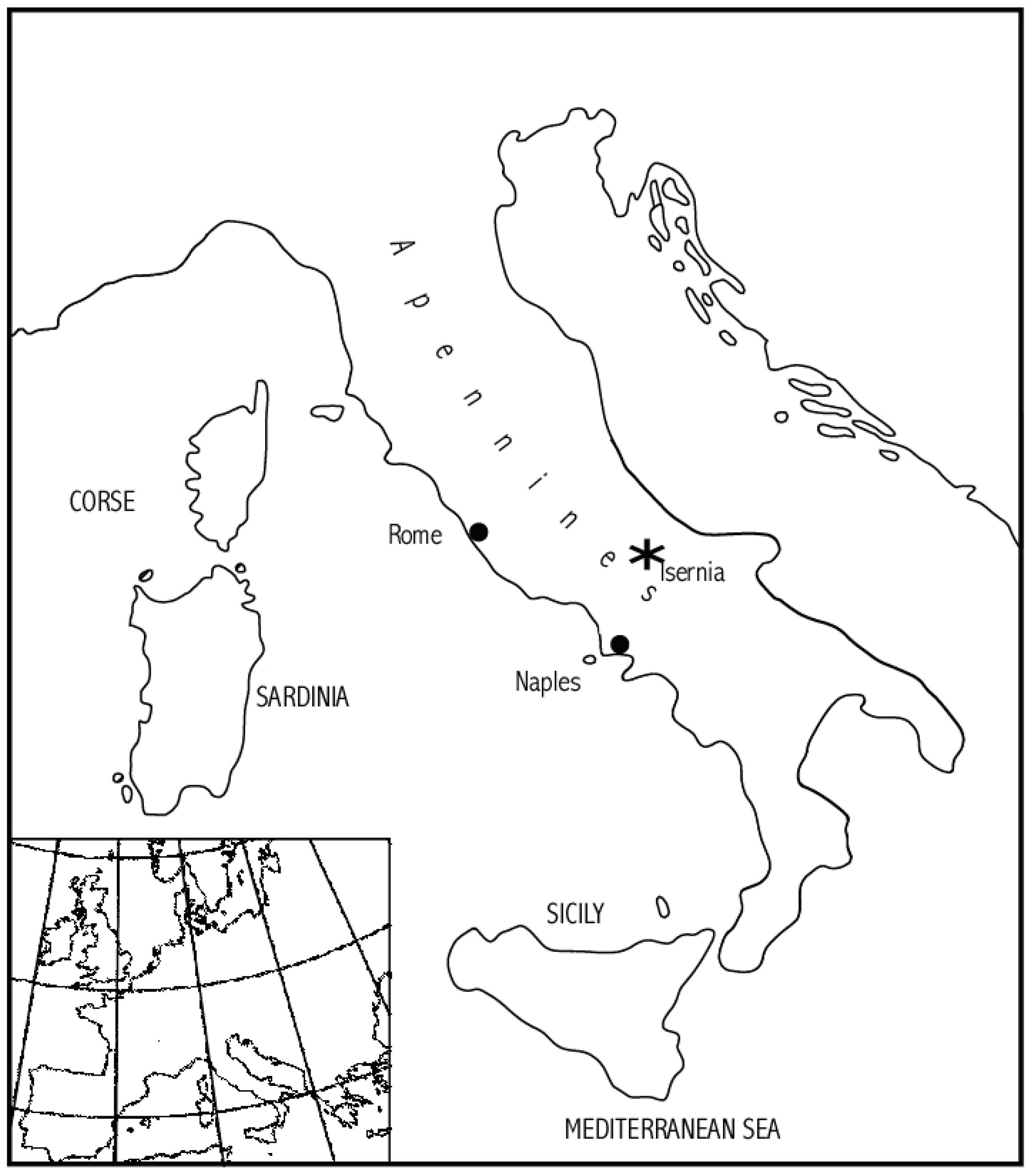
The value of the proposed measure is illustrated to the multiscale analysis of landscape changes taking place from 1954 to 2000 in the municipality of Isernia (Central Italy). The study area (6,874 ha in Central Italy; Figure 1) represents a pilot area of a larger research project aimed at analyzing the landscape dynamics of rural areas in Central Italy during 1950–2000 [16]. Altitudes range from 291 to 906 m a.s.l. Climate is temperate with warm and dry summers and cool winters.

Figure 1. Location of the study area.

Figure 1. Location of the study area.

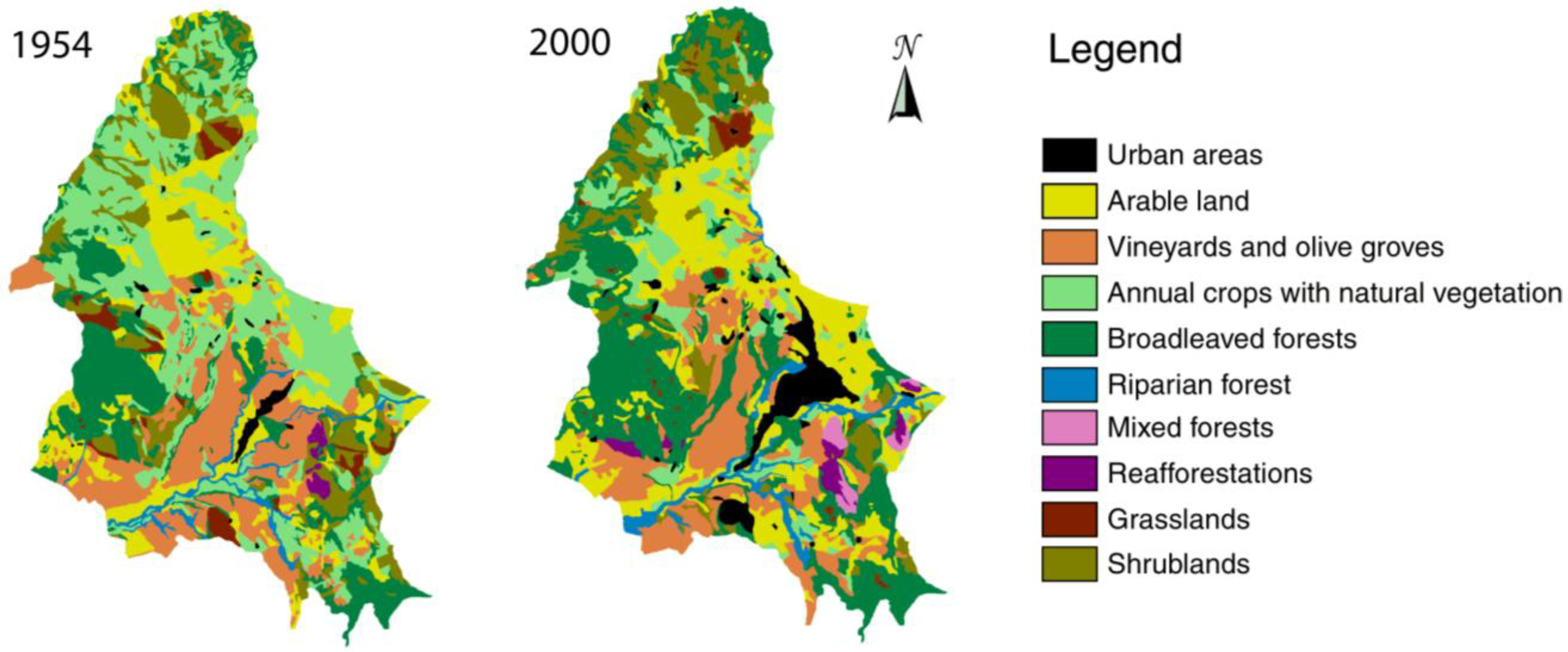
The municipality of Isernia consists of a small town of roughly 22,000 inhabitants surrounded by a hilly landscape with agricultural land cover in the alluvial plain and more natural LCCs at higher elevations. Using aerial photographs, two land cover maps (scale 1:25,000) of the study area were produced. Ten land cover classes were identified in the study area, and their distribution in 1954 and 2000 is shown in Figure 2.

Figure 2. Land cover maps of the study area in 1954 and 2000.

Figure 2. Land cover maps of the study area in 1954 and 2000.

In 1954, the study area can be described as a prevalently rural landscape constituted by a mosaic of annual crops together with olive groves and vineyards. At higher elevations, the dominant land cover classes were composed of natural and semi-natural vegetation types, such as extensive grasslands and broadleaved forests. In 2000, landscape heterogeneity tends to increase. Following the abandonment of the agro-silvo-pastoral practices in the least accessible areas, transitional shrublands became a significant constituent of the 2000 landscape. On the other hand, on lowlands and alluvial plains, traditional farming methods were extensively replaced by more intensive agricultural practices, leading to a homogenization of the former heterogeneous rural matrix into large crop fields. For a thorough analysis of the temporal dynamics of the study area, see [17].

The land cover maps of Figure 2 were overlaid with a series of grids composed of square boxes of a linear size of 10 m, 20 m, 40 m, 80 m, 160 m, 320 m, 640 m and 1,280 m, respectively. Next, the Rao index of each map was computed for each grid size. Among the many available measures of multivariate dissimilarity (see [18]), we calculated the pairwise dissimilarity, d_ij, between the different land cover combinations with the coefficient of Jaccard for the presence and absence data. Specifically, the Jaccard dissimilarity between two combinations of LCCs is obtained as the proportion of unshared LCCs out of the total number of LCCs recorded in both combinations: d_Jac = (b + c)/(a + b + c); where the letters refer to the traditional 2 × 2 contingency table: a is the number of LCCs shared by both combinations, b is the number of LCCs present in the first combination, but absent from the second combination, and c is the number of LCCs present exclusively in the second combination.

3. Results and Discussion

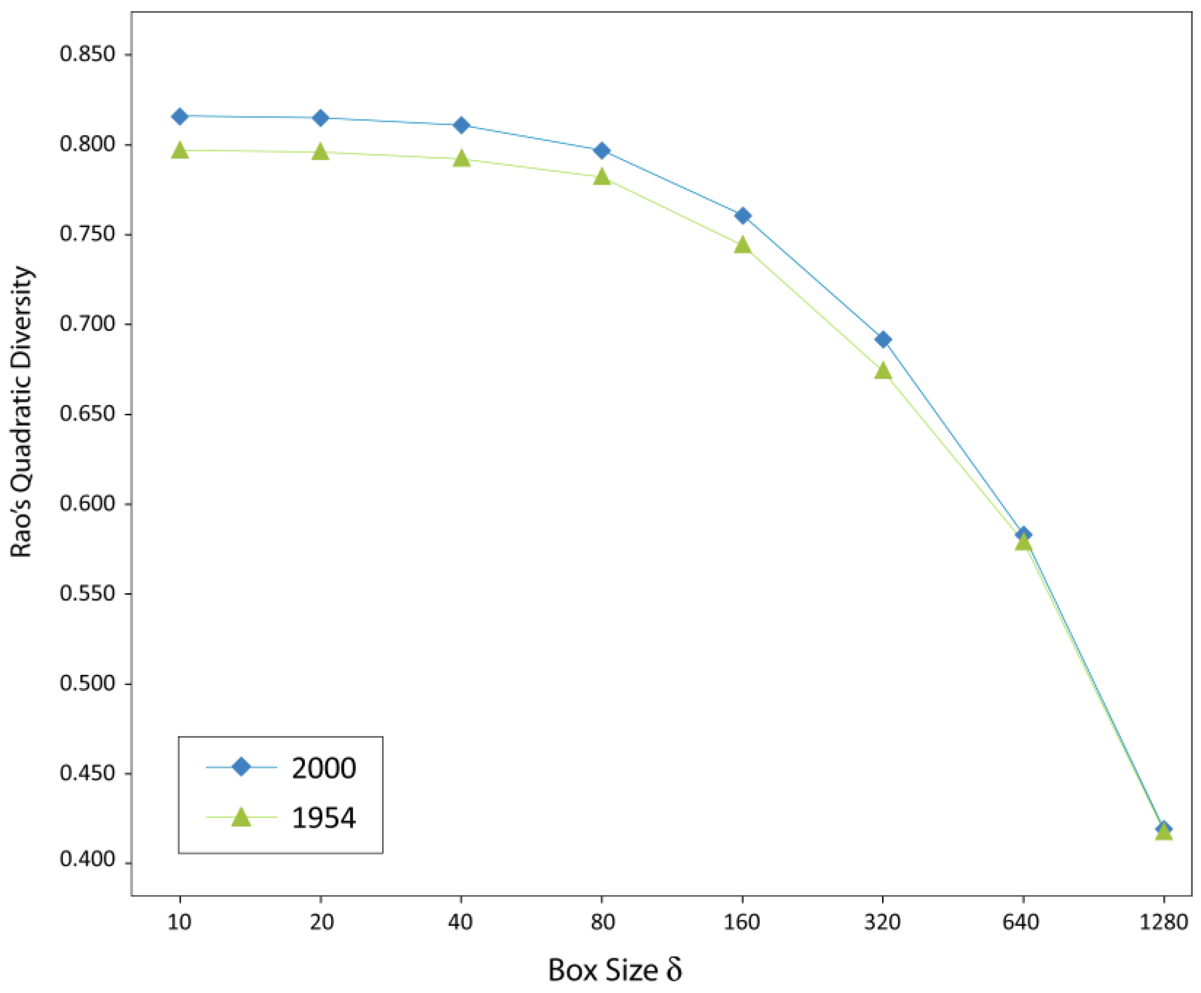
The plots of Q vs. box size, δ, for the land cover maps of Isernia in 1954 and 2000 extending from δ = 10 m up to δ = 1,280 m are shown in Figure 3 on a semi logarithmic scale. As shown in Figure 3, for both maps, the values of Q tend to decrease monotonically with box size. Although we were unable to mathematically prove the absence of local minima/maxima in the plots of Q vs.δ, nonetheless, the observed pattern seems intuitively reasonable: for small values of δ, most boxes contain only a few land cover types such that the proportion of LCCs shared by different combinations is usually low. Accordingly, for small box sizes, the expected distance between different LCC combinations is generally high. On the other hand, for very large boxes, the number of LCCs shared by different combinations is likely to increase, thus decreasing the values of Q. In spite of this general pattern, for small box sizes, the land cover map of 2000 is associated to the highest values of Q, and it is well separated from the map of 1954; for increasing values of δ, the differences between both landscapes tend to level out, and both curves are much closer to each other.

Figure 3. Plot of the Rao index Q vs. box size, δ, for the land cover maps of Isernia in 1954 and 2000 extending from δ = 10 m up to δ = 1,280 m.

Figure 3. Plot of the Rao index Q vs. box size, δ, for the land cover maps of Isernia in 1954 and 2000 extending from δ = 10 m up to δ = 1,280 m.

During 1954–2000, the region of Isernia experienced intense land cover changes that were mainly related to the marginalization of traditional agricultural practices due to ongoing socioeconomic shifts, like the aging and diminishing of the agricultural population, as more people become increasingly employed in manufacturing, construction and service sectors [16,19]. On alluvial plains, landscape changes are mainly related to the replacement of extensive agriculture and lowland forests (Quercus frainetto and Q. cerris woodlands) with more intensive agricultural practices. To the contrary, in less accessible areas, we face a general retrieval of shrublands and broadleaved forests (Quercus pubescens and Q. ilex woodlands) and a parallel decrease of pre-existing grasslands and olive groves. These processes, which are common to many other rural regions of Europe [20,21], will inevitably lead to a landscape homogenization in the long-term. However, in the short term, the fragmentation of lowland forests in the alluvial plains together with the natural vegetation dynamics at higher altitudes will both increase landscape fragmentation and heterogeneity. In this situation, the overall “compositional complexity” of the 2000 landscape is higher than for the 1954 landscape, especially for small box sizes. Unfortunately, we are not aware of any reliable method for generating confidence intervals for complex landscape indices. This makes significance testing of differences among various landscapes uncertain [22,23]. Nonetheless, the scale-dependent measure of compositional diversity proposed in this paper seems to reasonably portray the main changes in the study area during the period analyzed.

Given the direct relationship between Rao’s quadratic diversity and variance, the proposed method may be interpreted as an extension of block-size analysis of variance (ANOVA; see, e.g., [24]). In traditional block-size ANOVA, a quantitative (univariate) response variable is sampled within a gridded matrix. Next, contiguous quadrats are grouped in increasingly larger blocks (e.g., 2 × 2 quadrats, 4 × 4 quadrats, and so forth, until all grid cells have been summed to form the largest block size), and the variance at each block-size is computed. Plotting variance against block-size provides information on the scale-dependent pattern of the response variable, such that peaks in variance indicate clustering of quadrats, with high values of the response variable at that block-size.

In the proposed multivariate version, the most important methodological decision is about the method to be used to calculate dissimilarity, as the results obtained will depend to a certain extent on the multivariate measure, d_ij, used for quantifying the dissimilarity between the LCC combinations. Nonetheless, in spite of this source of uncertainty, as distinct measures were developed for summarizing different aspects of multivariate dissimilarity, we see this flexibility more as an advantage than a disadvantage, as it allows ecologists to compute relevant aspects of compositional complexity from different perspectives.

Finally, unlike traditional methods of landscape change analysis, which are usually based on transition matrices (see [25]), the number and frequency of the different combinations of LCCs in each map are not severely influenced by the co-registration accuracy of the underlying data sets. Accordingly, the proposed methodology may be reasonably adequate for analyzing historical data sets of varying resolution and quality, like aerial photographs or categorical maps.