Flood Susceptibility and Risk Assessment in Myanmar Using Multi-Source Remote Sensing and Interpretable Ensemble Machine Learning Model

Abstract

This observation-based and explainable approach demonstrates the applicability of multi-source remote sensing for flood assessment in data-scarce regions, offering a robust scientific basis for flood management and spatial planning in monsoon-affected areas. Floods are among the most frequent and devastating natural hazards, particularly in developing countries such as Myanmar, where monsoon-driven rainfall and inadequate flood-control infrastructure exacerbate disaster impacts. This study presents a satellite-driven and interpretable framework for high-resolution flood susceptibility and risk assessment by integrating multi-source remote sensing and geospatial data with ensemble machine-learning models—Extreme Gradient Boosting (XGBoost) and Light Gradient Boosting Machine (LightGBM)—implemented on the Google Earth Engine (GEE) platform. Eleven satellite- and GIS-derived predictors were used, including the Digital Elevation Model (DEM), slope, curvature, precipitation frequency, the Normalized Difference Vegetation Index (NDVI), land-use type, and distance to rivers, to develop flood susceptibility models. The Jenks natural breaks method was applied to classify flood susceptibility into five categories across Myanmar. Both models achieved excellent predictive performance, with area under the receiver operating characteristic curve (AUC) values of 0.943 for XGBoost and 0.936 for LightGBM, effectively distinguishing flood-prone from non-prone areas. XGBoost estimated that 26.1% of Myanmar’s territory falls within medium- to high-susceptibility zones, while LightGBM yielded a similar estimate of 25.3%. High-susceptibility regions were concentrated in the Ayeyarwady Delta, Rakhine coastal plains, and the Yangon region. SHapley Additive exPlanations (SHAP) analysis identified precipitation frequency, NDVI, and DEM as dominant factors, highlighting the ability of satellite-observed environmental indicators to capture flood-relevant surface processes. To incorporate exposure, population density and nighttime-light intensity were integrated with the susceptibility results to construct a natural–social flood risk framework. This observation-based and explainable approach demonstrates the applicability of multi-source remote sensing for flood assessment in data-scarce regions, offering a robust scientific basis for flood management and spatial planning in monsoon-affected areas.

1. Introduction

Floods are among the most frequent and destructive natural hazards worldwide, posing severe threats to agriculture, infrastructure, and human life [1]. According to the assessment report released by the United Nations Office for Disaster Risk Reduction (UNDRR) and the Centre for Research on the Epidemiology of Disasters (CRED, 2020), floods accounted for approximately 44% of all recorded natural disasters between 2000 and 2019, affecting more than 4 billion people and causing economic losses of about USD 2.97 trillion [2]. With the intensification of global warming and the increasing frequency of extreme rainfall events, flood hazards have become one of the most significant natural risks under climate change [3]. Developing countries, owing to their high climatic vulnerability and limited disaster-prevention capacity, are particularly exposed to flood impacts. Myanmar, located in the tropical monsoon region of Southeast Asia, is characterized by complex topography and a dense river network and is frequently affected by strong monsoon rainfall and tropical cyclones [4]. The catastrophic 2015 flood alone affected more than 1.6 million people and caused economic losses equivalent to 3.1% of the country’s GDP [5], underscoring the urgent need for effective large-scale flood assessment and risk management.

In flood-related studies, it is essential to distinguish between the concepts of flood hazard, flood susceptibility, and flood risk, as they represent different dimensions of flooding and are associated with distinct analytical approaches. Flood hazard refers to the probability of occurrence of a flood event with a given magnitude and frequency at a specific location in space and time and is commonly assessed using hydrological and hydraulic models that simulate flood extent, depth, and flow velocity under predefined scenarios. Flood susceptibility, by contrast, describes the inherent tendency of an area to be affected by flooding based on local environmental and territorial conditions, without explicitly considering event frequency or recurrence intervals. As emphasized by Varra et al. (2024), flood susceptibility analysis primarily aims to identify where flooding is more likely to occur, making it particularly suitable for large-scale assessments and for regions where detailed hydrological observations are limited [6]. Flood risk further extends these concepts by incorporating exposure and vulnerability, thereby reflecting the potential consequences of flooding for human activities and socioeconomic systems. In this study, flood risk is conceptualized as the integration of flood susceptibility and social exposure.

Flood susceptibility and flood risk assessment based on GIS and machine-learning techniques have been extensively investigated in recent years. Numerous studies have employed machine-learning models in combination with geomorphic, hydrological, and land-use-related factors to identify flood-prone areas across diverse geographical settings, including both data-rich and data-scarce regions [7]. Beyond susceptibility mapping, an increasing number of studies have incorporated socioeconomic or exposure-related indicators to support integrated flood risk assessment, highlighting the importance of linking physical flood-prone conditions with potential human impacts [8]. In parallel, recent studies have developed integrated or semi-automated assessment frameworks aimed at improving the scalability and transferability of flood risk analysis across different spatial contexts, such as multi-basin or large-area applications [9,10]. At the same time, cloud-based geospatial platforms, particularly Google Earth Engine (GEE, Google LLC, Mountain View, CA, USA), have been increasingly adopted to enable efficient processing of multi-source and multi-temporal datasets for regional- to national-scale flood assessment, especially in data-scarce environments [11,12]. Despite these advances, existing studies remain heterogeneous in terms of framework organization, validation strategies, and model interpretability, and flood susceptibility and flood risk components are often addressed using case-specific workflows, which limits cross-study comparability and large-scale application.

Within this context, this study develops and applies an integrated flood susceptibility and risk assessment framework to Myanmar as a representative data-scarce monsoon region. Rather than introducing new machine-learning algorithms, the focus of the study lies in the systematic design, large-scale implementation, and transparent evaluation of a unified and transferable workflow for national-scale flood assessment under limited ground-observation conditions. The specific objectives of this study are to: (1) develop a nationwide flood susceptibility assessment framework at high spatial resolution; (2) evaluate and compare the performance of XGBoost and LightGBM models; (3) interpret the relative contributions of natural and socioeconomic factors using SHAP; and (4) generate flood susceptibility and integrated risk maps to support flood disaster prevention and risk management in Myanmar and similar environments.

2. Materials and Methods

2.1. Overview of the Study Area

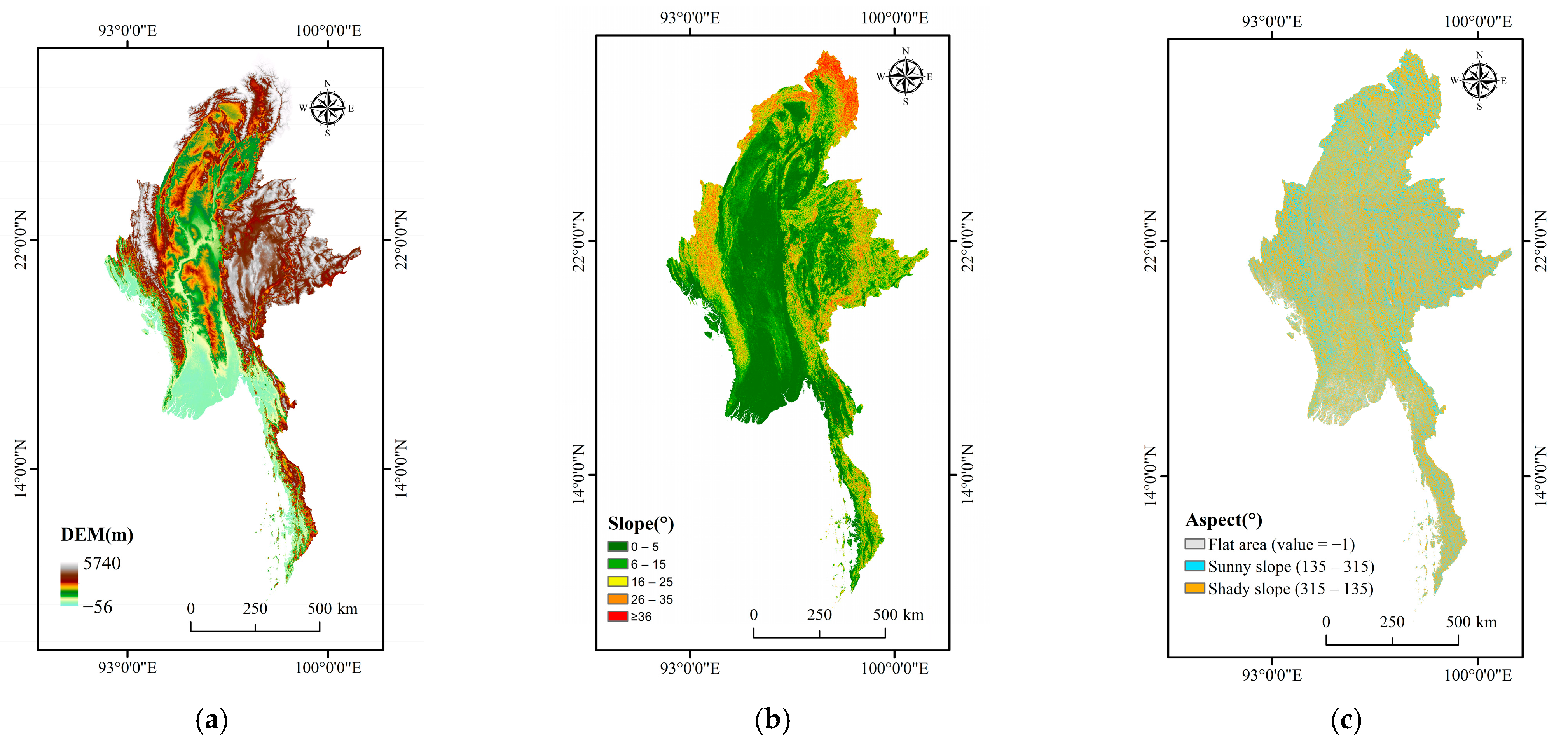
Myanmar is located in the western part of mainland Southeast Asia (9°32′ N–28°31′ N, 92°10′ E–101°11′ E), covering an area of approximately 676,578 km². The geographic location and elevation characteristics of the study area are shown in Figure 1.It is bordered by Thailand and Laos to the east, China to the north, India and Bangladesh to the northwest, and the Bay of Bengal and the Andaman Sea to the southwest. The country exhibits pronounced topographic heterogeneity, which strongly controls regional hydrological processes and flood characteristics. The northern and western regions are dominated by mountainous and plateau terrain, where steep slopes combined with intense monsoon rainfall frequently generate flash floods and rapid surface runoff. In contrast, the central lowlands, including the Ayeyarwady and Chindwin River basins, consist mainly of extensive alluvial plains that are regularly affected by seasonal river flooding. The southern Ayeyarwady Delta and coastal lowlands are characterized by very low elevations and are exposed to compound flood hazards resulting from river flooding, storm surges, and sea-level rise [13,14]. Myanmar has a typical tropical monsoon climate, with the main rainy season extending from May to October. Long-term observations indicate strong spatial variability in annual precipitation, exceeding 2000 mm in southern coastal areas, while central and northern regions generally receive between 1000 and 1500 mm per year. Consequently, floods occur frequently in the Ayeyarwady River Basin, causing substantial impacts on agricultural production, particularly in deltaic rice-growing areas that are highly sensitive to prolonged inundation [15]. The country has a population of approximately 55 million, more than 70% of whom reside in rural areas, many of which are located in flood-prone riverine and deltaic environments such as the Ayeyarwady Delta. Rapid urban expansion in major cities, including Yangon and Mandalay, has further intensified flood risk by increasing exposure and placing pressure on existing drainage and flood-protection infrastructure. Due to limited flood-control measures in rural regions and inadequate urban drainage systems, Myanmar exhibits high overall flood vulnerability, especially in densely populated low-lying areas [16]. Overall, the combination of complex topography, monsoon-dominated hydrological regimes, low-lying deltaic landscapes, and strong socio-economic dependence on river systems makes Myanmar a representative study area for large-scale flood susceptibility and flood risk assessment.

2.2. Data Sources and Data Preprocessing

2.2.1. Data Sources

To support the flood-susceptibility assessment in Myanmar, this study integrated a variety of high-resolution remote-sensing datasets and global geospatial databases covering topography, including topographic, meteorological, land-use, and river data; the Normalized Difference Vegetation Index (NDVI); historical flood imagery; and socioeconomic indicators such as population density and nighttime light intensity. All datasets were processed on the GEE platform where applicable, then reprojected to WGS_1984 (GCS_WGS_1984) and harmonized to a common analysis grid for modeling.

Table 1. Data Overview.

Data Type	Data Sources	Resolution/Year	Purpose	Acquisition Method
Topographic Data	ASTER GDEM V3 (30 m) Dataset	30 m/2020	Extract elevation, slope, aspect, TWI, SPI factors	http://www.Gscloud.cn (accessed on 1 October 2025)
Meteorological Data	UCSB-CHG/CHIRPSDataset	30 m/2020–2024	Extract annual precipitation frequency	Google Earth Engine Platform
Land Use Data	GLC_FCS30-2020	30 m/2020	Analyze the impact of 14 land cover types on flooding	https://data.casearth.cn (accessed on 1 October 2025)
River Data	HydroRIVERS (WWF) Global River Dataset [17]	30 m/2024	Extract river density and distance	https://hydrosheds.org (accessed on 1 October 2025)
NDVI	LANDSAT/LC08/C02/T1_L2 Dataset	30 m/2020–2024	Characterize vegetation cover status	Google Earth Engine Platform
Historical Flood Imagery	UNOSAT Flood Imagery	30 m/2020–2024	Flood extent calibration and model validation	https://unosat.org/products (accessed on 1 October 2025)
Socioeconomic Data	LandScan Global Population Database [18]	500 m/2024	Extract population density	https://landscan.ornl.gov (accessed on 1 October 2025)
	Global Scale Nightlight Time Series Dataset [19]	500 m/2024	Characterize socio-economic development level	https://github.com/eoatlas/nightlight (accessed on 1 October 2025)

summarizes the sources, resolutions, temporal coverage, purposes, and acquisition methods of each dataset.

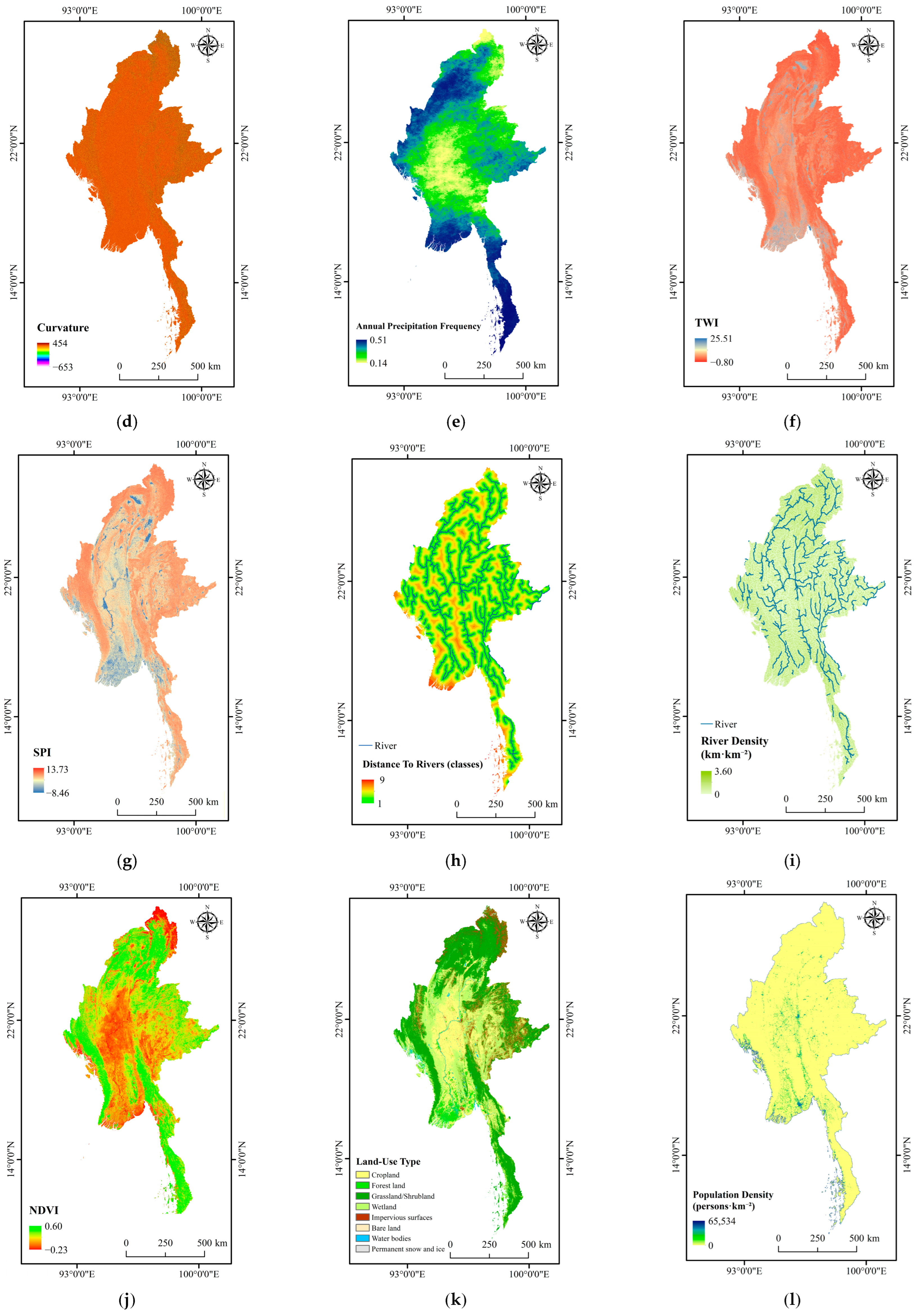
In selecting the influencing factors, eleven variables were identified based on flood-formation mechanisms and relevant literature [20,21,22,23]. The selection was guided by three primary criteria. First, the factors were required to represent the key physical processes governing flood generation and propagation, including topographic controls on runoff routing, meteorological forcing, drainage characteristics, land-surface conditions, and anthropogenic influences. Second, only variables that have been widely recognized as significant flood-conditioning factors in previous flood susceptibility and flood risk studies were considered, ensuring consistency with established research practices. Third, the number of influencing factors was constrained to balance explanatory completeness and model parsimony, thereby reducing redundancy and minimizing the risk of overfitting in machine-learning modeling. Based on these criteria, the selected influencing factors comprised the digital elevation model (DEM), slope, aspect, curvature, annual precipitation frequency, Topographic Wetness Index (TWI), Stream Power Index (SPI), distance to rivers, river density, Normalized Difference Vegetation Index (NDVI), and land-use type. All datasets were processed on the Google Earth Engine (GEE) platform where applicable, and resampled to a uniform 30 m grid to ensure spatial consistency, following recent remote-sensing studies that emphasize the importance of data harmonization and scale adaptation in heterogeneous environments [24]. Topographic variables were derived from the ASTER Global Digital Elevation Model (GDEM) v3 (30 m, 2020), which provides fine-resolution elevation data generated from stereo optical imagery collected by the Terra satellite. These topographic variables include the digital elevation model (DEM; Figure 2a) and its derivatives—slope (Figure 2b), aspect (Figure 2c), curvature (Figure 2d), Topographic Wetness Index (TWI; Figure 2f), and Stream Power Index (SPI; Figure 2g)—which together characterize terrain morphology and control the direction, velocity, and concentration of surface runoff, thereby influencing flood generation and propagation. Meteorological data were obtained from the Climate Hazards Group InfraRed Precipitation with Station (CHIRPS) dataset (30 m, 2020–2024), which combines satellite infrared estimates with in situ station observations. The derived annual precipitation frequency (Figure 2e), calculated from daily CHIRPS observations, represents the dominant hydrometeorological driver of flooding by describing the recurrence and intensity of rainfall events [25]. The CHIRPS dataset covers a five-year period. In terms of flood susceptibility, this concept focuses on characterizing the spatial tendency of an area to experience flooding under given environmental conditions. In this context, recent multi-year precipitation frequency provides sufficient information to capture spatial rainfall variability associated with flood-prone environments, particularly in data-scarce regions such as Myanmar. Hydrological indicators, including distance to rivers (Figure 2h) and river-network density (Figure 2i), were calculated using the HydroRIVERS Global River Dataset (WWF, 2024), which is based on the global river network framework developed by Lehner and Grill (2013) [20]. These indicators characterize drainage proximity and network connectivity, which, in combination with topographic and meteorological conditions, influence floodwater convergence and the spatial distribution of inundation across the study area. Vegetation characteristics were extracted from Landsat-8 Collection 2, Level 2 surface reflectance imagery (30 m, 2020–2024). The NDVI (Figure 2j), computed as (B5 − B4)/(B5 + B4), where B5 and B4 denote the near-infrared and red bands of Landsat-8, respectively, quantifies vegetation vigor and canopy density, which jointly reduce overland flow and mitigate soil erosion [26,27,28]. Land-use type (Figure 2k) information was obtained from the GLC_FCS30-2020 dataset (30 m, 2020), a globally consistent, fine-grained land-cover classification product based on Landsat imagery. To enhance interpretability, the original 14 categories were reclassified into eight representative classes: cropland, forest, grassland/shrubland, wetland, impervious surface, bare land, water body, and permanent snow and ice. These categories reflect variations in infiltration capacity and runoff potential across different surface types. Historical flood records were obtained from the UNOSAT Flood Extent Product (2020–2024), which provides satellite-derived flood footprints extracted from multispectral imagery for major flood events. These flood extent maps were used to construct an observation-based reference dataset representing historical flood occurrence across Myanmar. During the study period, UNOSAT flood extent products covering Myanmar were available for selected flood events in 2020, 2021, and 2024, while no official UNOSAT flood extent maps were released for 2022 and 2023. Specifically, the UNOSAT flood extent data were employed as an independent validation dataset to evaluate the spatial consistency and predictive performance of the flood susceptibility models. Flood and non-flood samples were derived by overlaying the model outputs with the satellite-observed inundation extents, allowing an objective comparison between predicted susceptibility patterns and observed flood occurrences. The spatial distribution of the UNOSAT flood extent products used in this study is illustrated in Figure 3. This validation strategy enables a robust assessment of model performance using ROC–AUC and related evaluation metrics (see Section 2.5), while avoiding reliance on sparse or unavailable ground-based flood records. The use of satellite-derived flood extents as an external validation reference is particularly suitable for large-scale flood susceptibility assessment in data-scarce regions such as Myanmar, where long-term and spatially continuous in situ flood observations are limited.

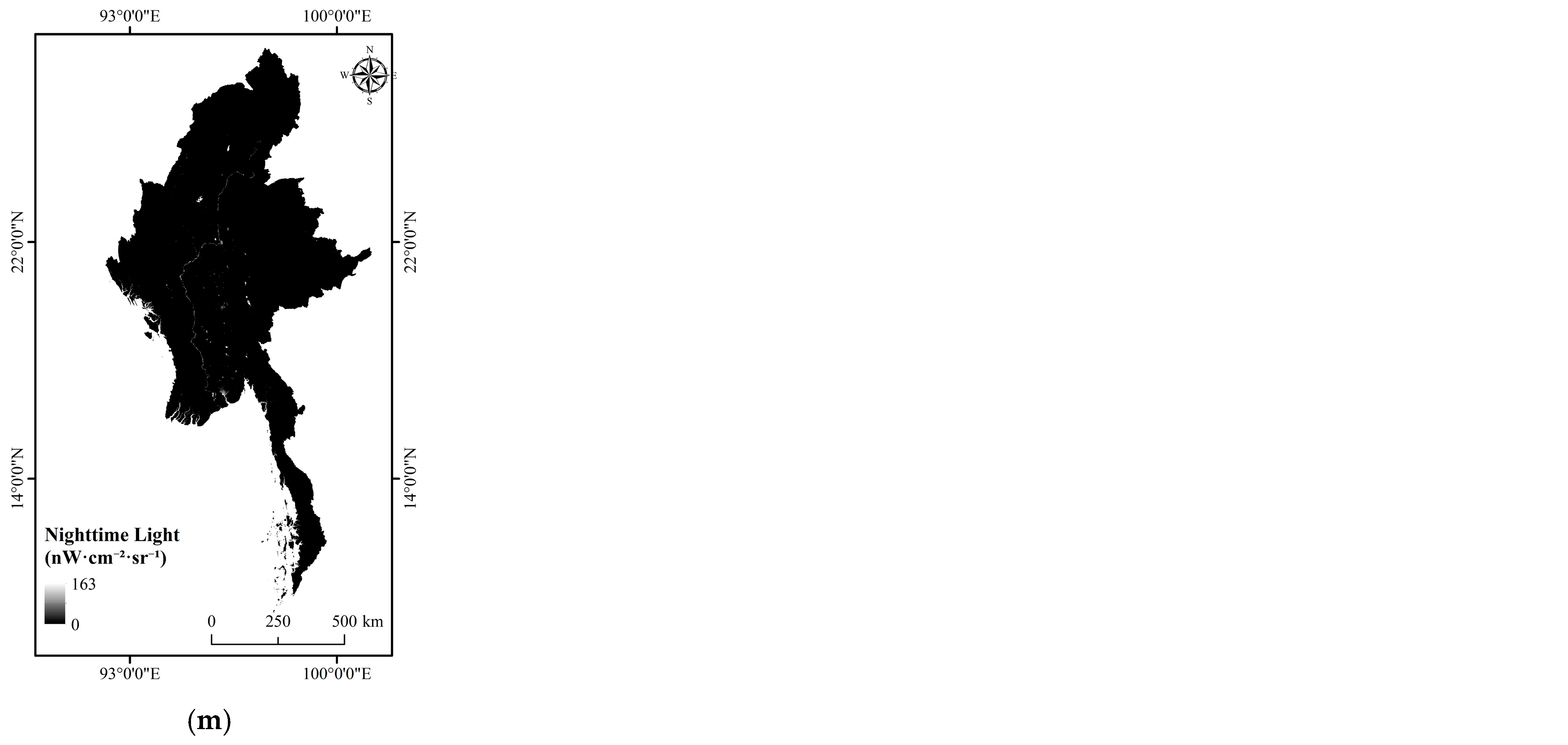
To represent anthropogenic exposure, two socioeconomic indicators were incorporated: population density, obtained from the LandScan Global Population Database (~500 m, 2024), and nighttime-light intensity, derived from the VIIRS Global Nighttime Light Series (~500 m, 2024). Population density (Figure 2l) captures the spatial concentration of human settlements, while nighttime light intensity (Figure 2m) serves as a remotely sensed proxy for economic activity and urbanization intensity. Collectively, these variables provide an integrated representation of the spatial heterogeneity of flood-related environmental and socioeconomic conditions across Myanmar.

2.2.2. Data Preprocessing

To ensure the quality of data sources and the consistency of model inputs, all datasets were systematically preprocessed through data cleaning, spatial registration, normalization, and multicollinearity analysis. The preprocessing was performed using ArcMap 10.8 (Esri, Redlands, CA, USA) and the GEE platform, with the objective of removing noise, standardizing data formats, and optimizing influencing factors to provide high-quality inputs for subsequent machine-learning modeling using XGBoost and LightGBM.

Table 2. Data Preprocessing Steps.

Preprocessing Step	Method/Tool	Description
Data Cleaning	Manual inspection/Linear interpolation (GEE)	Missing and abnormal values were removed. NDVI gaps caused by cloud cover were filled using linear interpolation. Incomplete socioeconomic records were excluded.
Spatial Registration	ArcMap 10.8	All datasets were reprojected to the GCS_WGS_1984 coordinate system and resampled to a spatial resolution of 30 m (except for population and nighttime light data).
Normalization	Min-max normalization	Influencing factors (e.g., DEM, Precipitation, NDVI) were scaled to a [0, 1] range to eliminate dimensional inconsistencies.
Multicollinearity Analysis	Pearson correlation coefficient/Variance Inflation Factor (VIF, Python 3.8)	Highly correlated influencing factors were identified using Pearson correlation analysis and VIF. Variables with |r| ≥ 0.75 or VIF > 10 were considered redundant and removed to reduce multicollinearity.

summarizes the preprocessing procedures and corresponding methods.

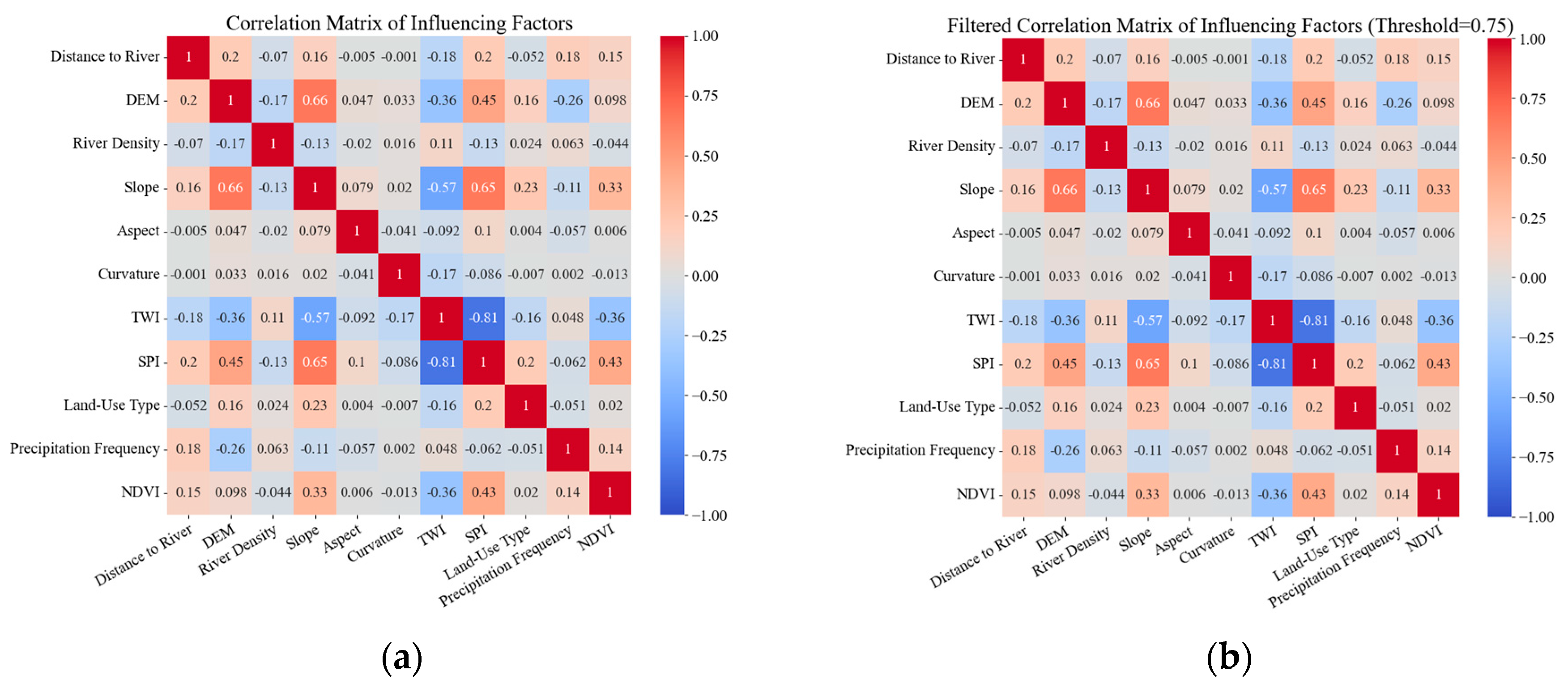
During the data-cleaning stage, missing and abnormal values were manually inspected and removed. For the NDVI dataset, cloud and shadow pixels were masked using the QA_PIXEL band, and temporal gaps caused by cloud cover were filled through linear interpolation on the Google Earth Engine (GEE) platform. Incomplete socioeconomic records were also excluded to maintain consistency across all datasets. For spatial harmonization, all datasets were reprojected to the Geographic Coordinate System WGS 1984 (GCS_WGS_1984) and resampled to a uniform 30 m spatial resolution. This process ensured pixel-level alignment across datasets, except for coarser-resolution layers such as the LandScan population (~500 m) and VIIRS nighttime light intensity (~500 m) data. Derived metrics, including annual precipitation frequency, population density, and nighttime light intensity, were first computed at their native resolutions and subsequently aligned to the 30 m analysis grid. This approach preserved spatial integrity while avoiding artificial upscaling artifacts. Subsequently, min–max normalization was applied to all continuous predictors (e.g., DEM, precipitation, NDVI) to scale their values within the [0, 1] range. This normalization removed unit inconsistencies among variables, thereby improving the numerical comparability and stability of the machine-learning models. Finally, a multicollinearity analysis was conducted using the Pearson correlation coefficient and the Variance Inflation Factor (VIF), computed in Python, to identify and remove highly correlated predictors. The Pearson correlation coefficient was used to detect strong pairwise linear relationships between variables, while VIF was employed to quantify multicollinearity in a multivariate context by measuring the degree to which the variance of a regression coefficient is inflated due to correlations with other predictors. An absolute Pearson correlation coefficient threshold of |r| ≥ 0.75 was adopted to indicate strong linear dependence between variable pairs, whereas a VIF value greater than 10 was used to identify severe multicollinearity. These threshold values are widely applied in multivariate statistical analysis and machine-learning studies to balance information retention and model stability [29,30]. Based on this analysis, the Stream Power Index (SPI) was excluded due to its strong negative correlation with the Topographic Wetness Index (TWI) (|r| = 0.81), indicating substantial redundancy between the two variables. TWI was retained as the representative terrain-related indicator because it more directly characterizes surface moisture accumulation and hydrological convergence processes relevant to flood generation. This filtering ensured that the remaining predictors were non-redundant, physically meaningful, and suitable for robust and interpretable flood-susceptibility modeling.

2.3. Technical Workflow

Based on the datasets and preprocessing procedures described in Section 2.2, a systematic five-stage technical workflow was established to integrate multi-source remote-sensing data with ensemble machine-learning models for large-scale flood susceptibility and flood risk assessment across Myanmar (Figure 4). The workflow was designed to ensure methodological transparency, logical consistency, and transferability, and comprises the following sequential stages: (1) Data acquisition and preprocessing. Multi-source environmental and socioeconomic datasets were collected and preprocessed using Google Earth Engine and ArcMap 10.8, with each platform applied according to its respective functionality. All datasets were subsequently harmonized in terms of spatial reference system, spatial resolution, and spatial extent to ensure consistency for subsequent modeling, following the procedures described in Section 2.2. (2) Influencing factor derivation. Flood-related influencing factors were derived from the preprocessed datasets. Dynamic variables, including precipitation frequency and NDVI derived from time-series satellite observations and representing temporally responsive environmental conditions, were incorporated together with static variables obtained through terrain and hydrological modeling to characterize the environmental controls on flood occurrence. (3) Dataset integration and multicollinearity screening. All influencing factors were standardized to a common spatial grid. To reduce redundancy and improve model stability, multicollinearity among variables was evaluated, and highly correlated predictors were excluded. The resulting dataset was then divided into training and validation subsets to support supervised machine-learning modeling. (4) Model training and evaluation. Two ensemble learning algorithms, XGBoost and LightGBM, were trained using the processed dataset. Model performance was assessed using multiple complementary statistical metrics to evaluate classification accuracy, robustness, and generalization capability. (5) Flood susceptibility prediction and mapping. Feature-importance analysis was applied to interpret the relative contribution of each influencing factor to flood susceptibility. The optimized models were subsequently used to generate high-resolution flood susceptibility maps, which were further integrated with exposure indicators to produce a comprehensive flood risk classification map. Overall, this workflow provides a coherent and transferable framework for integrating multi-source remote-sensing data, machine-learning modeling, and interpretability analysis, supporting large-scale flood susceptibility and flood risk assessment in data-scarce regions.

2.4. Machine-Learning Models

Building on the multi-source remote sensing and geospatial features described in Section 2.2, this study employs two ensemble learning algorithms based on gradient boosting—XGBoost and LightGBM—to model flood susceptibility. Both algorithms iteratively construct decision-tree ensembles and optimize a global objective function composed of a loss term and a regularization term, thereby enhancing predictive accuracy while effectively controlling model complexity and mitigating overfitting. In contrast to process-based hydrological or hydraulic models that explicitly simulate rainfall infiltration, runoff generation, and channel routing, the machine-learning models adopted in this study are designed to capture the integrated effects of hydrological processes through statistical learning from historical flood occurrences and multi-source remote sensing indicators. These indicators (e.g., precipitation frequency, DEM-derived terrain indices, NDVI, and distance to rivers) serve as effective proxies for key hydrological controls, including rainfall forcing, surface runoff convergence, moisture accumulation, and drainage conditions at a regional scale. Compared with conventional hydrological or statistical approaches, gradient-boosting models are well suited for modeling nonlinear relationships, handling high-dimensional feature spaces, and integrating heterogeneous remote sensing inputs [31]. These advantages make them particularly appropriate for large-scale flood susceptibility assessment in data-scarce regions. Although XGBoost and LightGBM share the same theoretical foundation, they differ in tree-growth strategies, feature-splitting mechanisms, and computational design, which affect their suitability under varying data scales and feature structures, as detailed below.

2.4.1. XGBoost

XGBoost is an ensemble learning method based on the gradient-boosting algorithm. Its main idea is to iteratively train multiple weak learners (usually decision trees) and optimize the model through a weighted approach, allowing subsequent learners to focus primarily on the samples misclassified by the previous round, thereby progressively improving overall prediction accuracy [32]. The objective function of XGBoost consists of a loss function and a regularization term, where the regularization term controls model complexity and prevents overfitting [33]. The objective function is defined as follows:

$$\mathsf{\Gamma }\left(\theta \right)={\displaystyle \sum _{i=1}^{n}L\left(y_i,{\widehat{y}}_i\right)}+{\displaystyle \sum _{k=1}^K\Omega \left(f_k\right)}$$

(1)

where $L\left(y_i,{\widehat{y}}_i\right)$ denotes the loss function, which measures the difference between the predicted and actual values. Common loss functions include mean squared error (MSE) and logarithmic loss (log loss). $f_k$ represents the k-th tree, and $\Omega \left(f_k\right)$ is the regularization term that constrains the complexity of the trees to avoid overfitting. The regularization term is defined as:

$$\Omega \left(f\right)=\gamma T+{\displaystyle \frac{1}{2}}\lambda {\displaystyle \sum _{j=1}^T{\omega }_j^2}$$

(2)

Here, $\gamma$ is the regularization parameter that penalizes model complexity, $T$ denotes the number of leaf nodes in the tree, ${\omega }_j$ represents the weight of the j-th leaf node, and $\lambda$ is the regularization coefficient that controls the magnitude of leaf weights. Introducing the regularization term effectively prevents overfitting and enhances the model’s generalization ability.

For flood-risk prediction, XGBoost effectively captures the nonlinear interactions among remote-sensing-derived factors, including precipitation frequency, elevation (DEM), slope, aspect, curvature, topographic wetness index (TWI), and stream power index (SPI), as well as other environmental and socioeconomic indicators. Its strong regularization and tree-based architecture ensure stable performance in medium-scale datasets characterized by spatial heterogeneity and moderate noise. However, when applied to very large study areas or extremely dense feature sets, XGBoost tends to incur higher computational and memory costs, leading to longer training times. Overall, XGBoost demonstrates excellent predictive performance in flood-risk assessment tasks with complex feature dimensions but moderate sample sizes, effectively reducing prediction errors and outperforming traditional statistical approaches across multiple evaluation metrics [34].

2.4.2. LightGBM

LightGBM is an efficient gradient boosting framework that is particularly suitable for handling large-scale datasets and high-dimensional features. Its main innovation lies in employing a histogram-based algorithm to accelerate the tree-building process and adopting a leaf-wise growth strategy to optimize tree structure [35]. This significantly improves computational efficiency, especially when processing high-dimensional and multi-class flood-related data [36]. The objective function of LightGBM is similar to that of XGBoost, but it utilizes different tree growth strategies and computational methods. The objective function can be expressed as follows:

$$\mathsf{\Gamma }\left(F\right)={\displaystyle \sum _{i=1}^{n}L\left(y_i,F\left(x_i\right)\right)}+{\displaystyle \sum _{k=1}^K\Omega \left(f_k\right)}$$

(3)

where $L\left(y_i,F\left(x_i\right)\right)$ denotes the loss function, and $\Omega \left(f_k\right)$ represents the regularization term. Unlike XGBoost, LightGBM uses a histogram-based splitting strategy, which reduces computational overhead and accelerates training. This enables the algorithm to efficiently handle large-scale and sparse datasets [35].

In remote-sensing applications, LightGBM efficiently processes massive gridded datasets, making it particularly suitable for national- or regional-scale flood mapping. It accelerates training through Gradient-based One-Side Sampling (GOSS) and supports categorical feature handling, which facilitates the integration of diverse data types—such as land-use categories, spectral indices, and topographic metrics—within a unified learning framework. Empirically, LightGBM achieves comparable or even superior predictive accuracy to XGBoost, while requiring substantially less computational time, enabling rapid model optimization and scenario analysis for large-scale studies.

In summary, both models are applied independently and in parallel in remote-sensing-based flood-susceptibility modeling, rather than being integrated into a single hybrid framework. XGBoost provides stronger regularization and interpretability for medium-scale datasets with complex but controlled feature dimensions, whereas LightGBM delivers superior scalability and efficiency for large-area, high-resolution remote-sensing applications. By comparing the two models under the same data and feature settings, this study aims to assess the consistency and robustness of flood susceptibility patterns, thereby ensuring stable, reproducible, and operationally applicable predictions for large-scale flood-risk mapping and management.

2.5. Performance Evaluation Metrics and Validation Strategy

Rigorous evaluation of model performance is essential to ensure the reliability of flood-risk predictions across Myanmar, particularly given the heterogeneous and class-imbalanced nature of the dataset. Therefore, multiple complementary statistical metrics were employed to provide a comprehensive assessment of model performance. The full dataset was randomly divided into a training set (70%) and an independent validation set (30%), and model performance was evaluated using the Receiver Operating Characteristic curve and Area Under the Curve (ROC–AUC), Precision, Recall, F1-score, Jaccard index, and adjusted accuracy. Model evaluation was conducted based on flood and non-flood samples derived from satellite-observed flood records. Flood samples (positive class) were obtained from the UNOSAT Flood Extent Product (2020–2024), with grid cells identified as inundated during observed flood events labeled as positive samples. Non-flood samples (negative class) were randomly selected from areas outside the mapped flood extents, excluding buffer zones surrounding observed flood areas to reduce uncertainty associated with the absence of flooding. Based on these labeled samples, true positives, true negatives, false positives, and false negatives were determined by comparing model predictions with observed flood occurrences.

2.5.1. Precision

Precision measures the proportion of correctly predicted positive samples among all samples predicted as positive. In flood risk prediction, precision reflects the model’s ability to accurately identify areas that are truly at risk of flooding when they are classified as flood-prone regions [37]. The calculation formula is expressed as:

$$Precision={\displaystyle \frac{TP}{TP+FP}}$$

(4)

where $TP$ (True Positive) denotes the number of samples correctly predicted as positive, and $FP$ (False Positive) represents the number of negative samples incorrectly predicted as positive.

2.5.2. Recall

Recall quantifies the proportion of correctly identified positive samples among all actual positive samples (i.e., regions where flooding truly occurred). A higher recall value indicates that the model can detect a larger proportion of potential flood-risk areas. In flood disaster risk assessment, improving Recall contributes to the timely identification of flood hazards and the implementation of preventive measures. The calculation formula is given as:

$$Recall={\displaystyle \frac{TP}{TP+FN}}$$

(5)

where $FN$ (False Negative) refers to the number of positive samples incorrectly predicted as negative. A higher recall indicates a lower risk of missed detections, effectively reducing the likelihood of overlooking real flood-prone regions [38].

2.5.3. F1-Score

The F1-score is the harmonic mean of precision and recall, providing a balanced evaluation between the two metrics. In flood disaster risk assessment, the F1-score serves as a comprehensive performance indicator that reflects the trade-off between precision and recall. It is particularly valuable when dealing with class-imbalanced datasets, as it provides a more objective measure of model performance. The calculation formula is as follows:

$$F1=2\times {\displaystyle \frac{Precision\times Recall}{Precision+Recall}}$$

(6)

The F1-score ranges from 0 to 1, with higher values indicating a better balance between precision and recall. Therefore, in flood-risk prediction, the F1-score is an important integrated metric for evaluating overall model performance [33].

2.5.4. Accuracy

Accuracy is the most intuitive evaluation metric, representing the proportion of correctly predicted samples among all samples. It reflects the overall correctness of model predictions across both positive and negative classes. The formula for Accuracy is given as:

$$Accuracy={\displaystyle \frac{TP+TN}{TP+TN+FP+FN}}$$

(7)

where $TP$ (True Positive) refers to the number of correctly predicted positive samples, $TN$ (True Negative) denotes the number of correctly predicted negative samples, $FP$ (False Positive) is the number of negative samples incorrectly predicted as positive, and $FN$ (False Negative) represents the number of positive samples incorrectly predicted as negative [37]. Although accuracy is an important indicator, it may fail to adequately represent model performance in class-imbalanced scenarios; therefore, it should be used in conjunction with other evaluation metrics.

2.5.5. ROC Curve

The Receiver Operating Characteristic Curve (ROC Curve) depicts the relationship between the False Positive Rate (FPR) and the True Positive Rate (TPR, i.e., recall) across varying classification thresholds, providing an overall view of model behavior. The Area Under the Curve (AUC) quantifies the model’s ability to distinguish between positive and negative samples. An AUC value closer to 1 indicates stronger discriminative capability; when AUC = 0.5, the model performs the same as random guessing. In flood disaster risk prediction, AUC offers a comprehensive measure of overall performance and remains particularly informative under class-imbalanced conditions [39].

2.5.6. Jaccard Index

The Jaccard Index quantifies the overlap between the predicted positive and ground-truth positive sets; higher values indicate greater agreement between predictions and observations. It is computed as

$$Js={\displaystyle \frac{TP}{TP+FP+FN}}$$

(8)

In flood-risk prediction, a higher Jaccard Index signifies more accurate localization of flood-prone areas. Importantly, the Jaccard Index assesses the quality of positive-class detection rather than overall accuracy; under class imbalance, it is typically more informative than accuracy for evaluating the model’s discrimination and spatial targeting capability [40].

2.5.7. Adjusted Accuracy

Adjusted Accuracy takes into account the effects of class imbalance and other factors that may bias traditional accuracy measures. It provides a more objective assessment of model performance under complex sample distributions [41]. The formula is given as:

$$Adj.Acc={\displaystyle \frac{Norm\mp \left({\delta }^1,{\delta }^2\dots {\delta }^{\infty }\right)}{{\displaystyle \sum N}}}$$

(9)

where $\delta$ denotes the accuracy metric, and N represents the total number of accuracy indicators considered. This adjusted form ensures a fairer evaluation of model performance across unevenly distributed categories in flood risk assessment.

2.6. SHAP-Based Feature Importance Analysis Methodology

In flood-susceptibility modeling, the “black-box” nature of machine-learning algorithms often limits the interpretability of their prediction mechanisms. To improve model transparency and interpretability, this study employed the SHapley Additive exPlanations (SHAP) method to quantify feature importance for both the XGBoost and LightGBM models. Based on Shapley values, SHAP assigns an importance score to each feature, quantifying its contribution to the model output and allowing consistent and explainable interpretation of model behavior [42].

To ensure the reliability of the feature-importance analysis, all variables were standardized and preprocessed to minimize potential bias caused by data quality, scale differences, and multicollinearity. The analysis results were visualized using two complementary tools: the Summary Plot and the Force Plot. The Summary Plot provides a global overview of feature influence, ranking variables according to their overall contribution to model predictions. The Force Plot focuses on individual predictions, illustrating how each feature drives a specific model output. By combining these two visualization approaches, the SHAP analysis provides a clear understanding of the key factors influencing flood susceptibility and enhances the interpretability of model predictions. This strengthens the analytical foundation of the study and supports subsequent flood-risk assessment and decision-making [43,44].

3. Results

3.1. Correlation Analysis of Influencing Factors

To minimize the potential impact of multicollinearity on the performance and stability of the XGBoost and LightGBM models, the influencing factors were screened using a combination of Pearson correlation coefficient analysis and Variance Inflation Factor (VIF) assessment (Figure 5). Pearson correlation analysis was first applied to quantify the linear relationships among the eleven influencing factors. Following commonly adopted practices in environmental modeling and machine-learning studies, a correlation threshold of |r| ≥ 0.75 was used to identify highly correlated variable pairs, as values exceeding this threshold generally indicate strong linear dependence and potential redundancy among predictors. The analysis revealed that the Topographic Wetness Index (TWI) and the Stream Power Index (SPI) exhibited a strong negative correlation (r = −0.81). Because both indices are derived from similar topographic attributes and describe closely related hydrological processes associated with surface runoff and flow concentration, retaining both variables could introduce redundancy into the model. To reduce multicollinearity while maintaining physical interpretability, SPI was excluded, and TWI was retained as the representative variable due to its more direct relevance to soil moisture accumulation and surface saturation processes involved in flood generation. After the removal of SPI, Pearson correlation analysis was recalculated for the remaining influencing factors. All pairwise correlation coefficients were below the selected threshold, indicating acceptable independence among predictors. Subsequently, VIF analysis was conducted to further assess multicollinearity and model stability. A VIF threshold of 10 was adopted in accordance with widely used guidelines in regression-based and machine-learning applications, where values exceeding this threshold typically indicate severe multicollinearity. The results showed that all retained variables had VIF values below 10, confirming the absence of significant multicollinearity and validating the reliability of the final feature set for subsequent model training.

3.2. Evaluation of Predictive Performance

3.2.1. Comparison of Model Performance

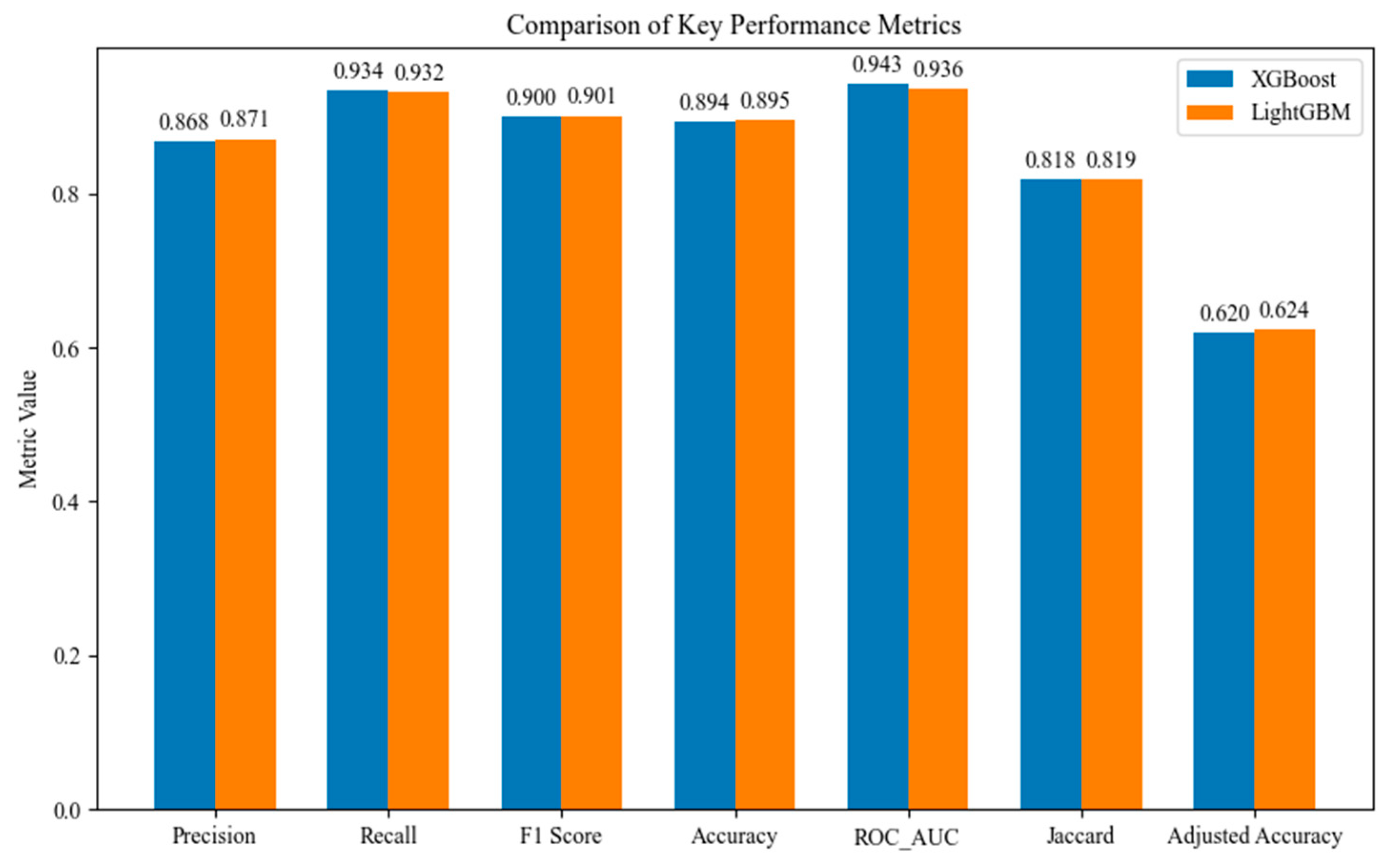
To comprehensively evaluate the performance of the constructed models in flood disaster risk prediction, this study conducted a multi-metric comparison between the XGBoost and LightGBM algorithms, as illustrated in Figure 6. The evaluation metrics include Precision, Recall, F1-Score, Accuracy, ROC_AUC, Jaccard coefficient, and Adjusted Accuracy, which collectively reflect the models’ recognition ability and stability from multiple perspectives. In terms of Precision, LightGBM (0.871) slightly outperformed XGBoost (0.868), indicating a marginally better capability in reducing false positives. Regarding Recall, XGBoost (0.934) achieved a slightly higher value than LightGBM (0.932), suggesting that XGBoost has a advantage in identifying actual flood-affected areas. The F1-Score (0.901 for LightGBM and 0.9 for XGBoost) further confirms the superior balance of LightGBM between precision and recall. Although the difference in Accuracy (0.895 for LightGBM and 0.894 for XGBoost) is relatively small, LightGBM demonstrated more consistent overall performance. In the comparison of ROC_AUC values (0.943 for XGBoost and 0.936 for LightGBM), XGBoost exhibited a slightly stronger ability to distinguish between flood-risk and non-risk areas. Both models showed highly similar performance in the Jaccard coefficient (0.819 for LightGBM and 0.818 for XGBoost), indicating substantial overlap in the identification of actual flood-risk regions. Regarding Adjusted Accuracy, LightGBM (0.624) outperformed XGBoost (0.620), highlighting its advantage in handling class imbalance. Overall, while XGBoost exhibited marginal superiority in certain metrics, LightGBM performed more consistently across most evaluation criteria. Its balanced performance, especially under large-scale data and complex scenarios, underscores its higher predictive accuracy and robustness.

3.2.2. Confusion Matrix Analysis

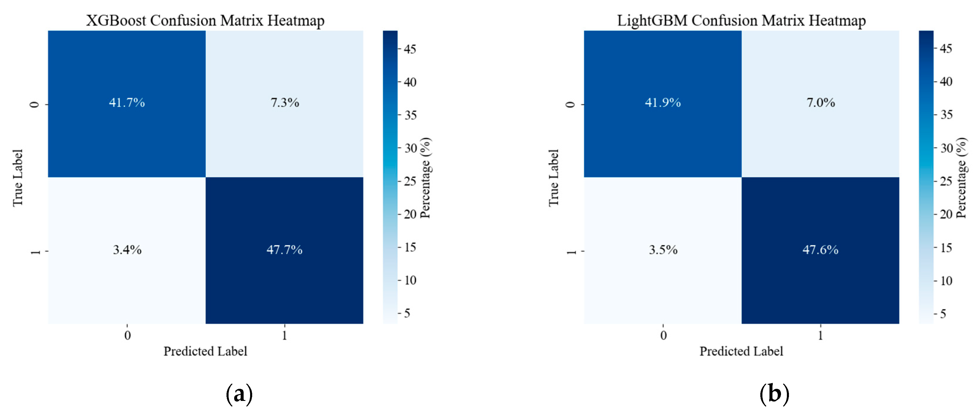
To further evaluate the classification performance of the models in flood-risk prediction, a comparative analysis of the confusion matrices for XGBoost and LightGBM was conducted (Figure 7). The results show that XGBoost correctly identified approximately 47.7% of high-risk flood areas, while LightGBM achieved a similar detection rate of 47.6%, indicating that both models effectively captured flood-prone regions. Regarding misclassifications, the false positive rate (FPR) of XGBoost was around 7.3%, compared with 7.0% for LightGBM, suggesting that LightGBM has a slightly stronger capability to reduce the incorrect identification of non-risk areas as high-risk zones. The difference in false negative rates (FNR) between the two models was minimal (approximately 3.4–3.5%), indicating comparable sensitivity in detecting actual flood-affected areas. Overall, LightGBM exhibited marginally better performance in minimizing misclassification errors, particularly in reducing false positives, which helps prevent unnecessary over-warning of non-risk areas in practical flood-risk assessments. Meanwhile, XGBoost demonstrated strong classification capability and stable predictive behavior, confirming that both ensemble-learning algorithms are reliable and suitable for flood-risk identification and spatial prediction.

3.2.3. ROC Curve Analysis

The performance of the XGBoost and LightGBM models was further validated through ROC curve analysis, as presented in Figure 8. The results show that the AUC value of XGBoost reached 0.943, slightly higher than that of LightGBM (0.936). Both values are substantially greater than the AUC of random guessing (0.5), indicating excellent discriminative capability in flood-risk identification based on multi-source environmental and topographic variables. From the perspective of factor contribution, the DEM, slope, and TWI exhibited relatively high AUC values, underscoring their dominant influence on flood-susceptibility modeling. In particular, the DEM strongly affects surface-water accumulation and drainage patterns—high-elevation areas tend to drain more efficiently, while low-lying areas are prone to water retention and flooding. The slope and TWI further regulate flood potential by influencing runoff velocity and soil-moisture distribution. Additionally, factors such as distance to rivers, land-use type, precipitation frequency, and NDVI showed moderate discriminative ability. Among them, the proximity to rivers and precipitation frequency are directly related to flood occurrence, making them key predictive indicators. In contrast, river density, aspect, and curvature yielded relatively lower AUC values, possibly due to regional differences in geomorphological and hydrological conditions. Overall, both XGBoost and LightGBM demonstrated excellent predictive performance, effectively delineating flood-prone areas using integrated geospatial and remotely derived features. The high AUC values confirm that both models are robust and reliable for large-scale flood-susceptibility assessment.

3.3. Feature Importance Analysis

3.3.1. Evaluation of Feature Importance

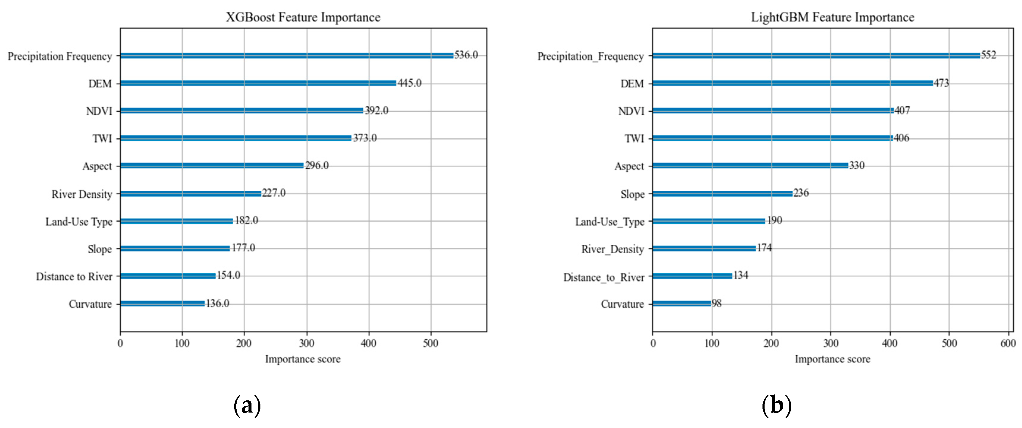
To systematically evaluate the contribution of environmental variables to flood susceptibility modeling, a feature importance analysis was conducted using both the XGBoost and LightGBM algorithms (Figure 9). The two models exhibited a high degree of consistency in identifying the principal determinants of flood occurrence. Precipitation frequency, elevation (DEM), and vegetation index (NDVI) emerged as the dominant predictors, representing the hydrometeorological, geomorphological, and ecological controls on flood generation. Although the overall ranking of variable importance was consistent between the two algorithms, LightGBM demonstrated slightly higher sensitivity to terrain-related parameters such as slope and aspect, suggesting its greater ability to capture micro-topographic variability under complex surface conditions. This finding indicates that LightGBM provides a more refined representation of landscape heterogeneity, enhancing the interpretability of its predictive mechanism in physical terms. Collectively, the results confirm that precipitation, topography, and vegetation are the fundamental environmental drivers of flood susceptibility in the study region. The convergence of importance patterns across both ensemble models validates the robustness of the identified predictors and underscores the effectiveness of integrating multi-source environmental variables within ensemble learning frameworks to achieve more reliable, interpretable, and spatially coherent flood risk predictions.

3.3.2. Analysis of Model Predictive Power

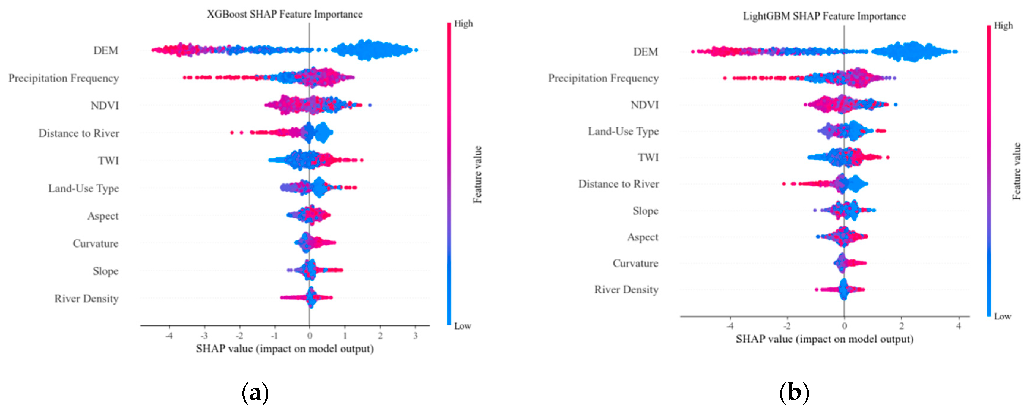
To enhance the understanding of the models’ decision-making mechanisms, this study utilized the SHAP method to analyze the predictive power of XGBoost and LightGBM. SHAP values quantify the marginal contribution of each feature to the model output, revealing both positive and negative influences, thus enabling interpretability analysis at both global and individual levels.

At the global feature level (Figure 10), both models consistently identified DEM, precipitation frequency, and NDVI as the primary drivers of flood susceptibility. The SHAP results confirm that elevation and rainfall-related variables exert the strongest influence, while vegetation cover contributes negatively to flood probability. Other factors such as TWI, land use, and proximity to rivers also showed moderate contributions, indicating secondary yet meaningful influences on model prediction. In contrast, slope, curvature, and river density exhibited comparatively lower importance, suggesting limited impact on overall susceptibility under regional conditions.

At the local feature level (Figure 11), the SHAP explanations reveal that XGBoost and LightGBM maintain similar directional effects across individual predictions but differ in the magnitude with which specific predictors influence their outputs. XGBoost exhibits a stronger reliance on terrain-driven factors, with elevation, NDVI, precipitation frequency, and particularly curvature contributing prominently to its positive local prediction. In addition, distance to rivers imposes the most substantial negative effect, indicating heightened responsiveness to drainage proximity and terrain geometry. In contrast, LightGBM places greater emphasis on precipitation–vegetation interactions and surface conditions. NDVI and precipitation frequency remain among its strongest positive contributors, while land-use type, slope, and curvature exert comparatively higher influences than in XGBoost. Meanwhile, the negative effect of distance to rivers is weaker, suggesting reduced sensitivity to near-channel hydrological gradients.

A comparison of the models (Figure 12) further demonstrated that both models identified core features consistently, but differed in their feature dependence. LightGBM showed higher overall reliance on DEM, precipitation frequency, and NDVI, suggesting that it is more capable of explaining the combined effects of topographic variation, precipitation characteristics, and vegetation cover on flood risk. In contrast, XGBoost exhibited a stronger response to distance to rivers, aspect, and features such as slope, curvature, and river density, indicating its relative advantage under complex terrain and flow accumulation conditions.

Overall, the SHAP analysis validates the dominant role of hydrological factors (precipitation and river conditions), topographic features (elevation and terrain variation), and vegetation cover in flood-susceptibility prediction across both global and local scales. The models also demonstrate complementary feature sensitivities: LightGBM better reflects precipitation- and vegetation-driven risk patterns, whereas XGBoost provides stronger interpretability in terrain- and drainage-controlled scenarios. This complementarity enhances the robustness of the analysis and offers valuable guidance for model selection and feature configuration in diverse environmental settings.

3.4. Spatial Distribution of Flood Susceptibility

Based on the flood susceptibility indices derived from the XGBoost and LightGBM models, Myanmar was classified into five flood susceptibility levels using the Natural Breaks (Jenks) method. The susceptibility index is a continuous variable ranging from 0 to 1, and the Jenks algorithm was applied to identify statistically optimal class breakpoints based on the data distribution. The resulting classes correspond approximately to low (0–0.2), moderately low (0.2–0.4), moderate (0.4–0.6), moderately high (0.6–0.8), and high (0.8–1.0) susceptibility levels, enabling a clear and interpretable representation of spatial variability across the country. The XGBoost-based results (Figure 13a) indicate that 67.5% of Myanmar falls within the low-susceptibility category, followed by 6.4% classified as moderately low, 4.7% as moderate, 5.8% as moderately high, and 15.6% as high susceptibility. Overall, approximately 26.1% of the national territory is characterized by moderately high to high flood susceptibility. These areas are mainly concentrated in the Ayeyarwady River Basin and Delta, the Rakhine coastal plains, and the Yangon region, where low elevation, dense river networks, and frequent monsoon rainfall jointly contribute to elevated flood susceptibility. The LightGBM model produces a highly comparable spatial pattern (Figure 13b). Low-susceptibility areas account for 70.5% of the country, while 4.2%, 3.2%, 3.7%, and 18.4% of the area fall into the moderately low, moderate, moderately high, and high susceptibility classes, respectively. In total, 25.3% of Myanmar is classified as moderately high or high susceptibility. Consistent with the XGBoost results, these high-susceptibility zones are predominantly located in the Ayeyarwady Delta and coastal lowlands, reflecting the combined influence of terrain conditions, hydrological connectivity, and precipitation intensity. Despite minor differences in the proportional extent of susceptibility classes, both models exhibit nearly identical spatial distribution patterns. They consistently identify the Ayeyarwady Delta, Rakhine coastal plains, and Yangon lowlands as the most flood-prone regions in Myanmar. This strong agreement between models indicates robust predictive performance and confirms that flood susceptibility across the country is primarily governed by the integrated effects of topography, monsoon-driven rainfall, and river network structure.

3.5. Flood Disaster Risk Assessment

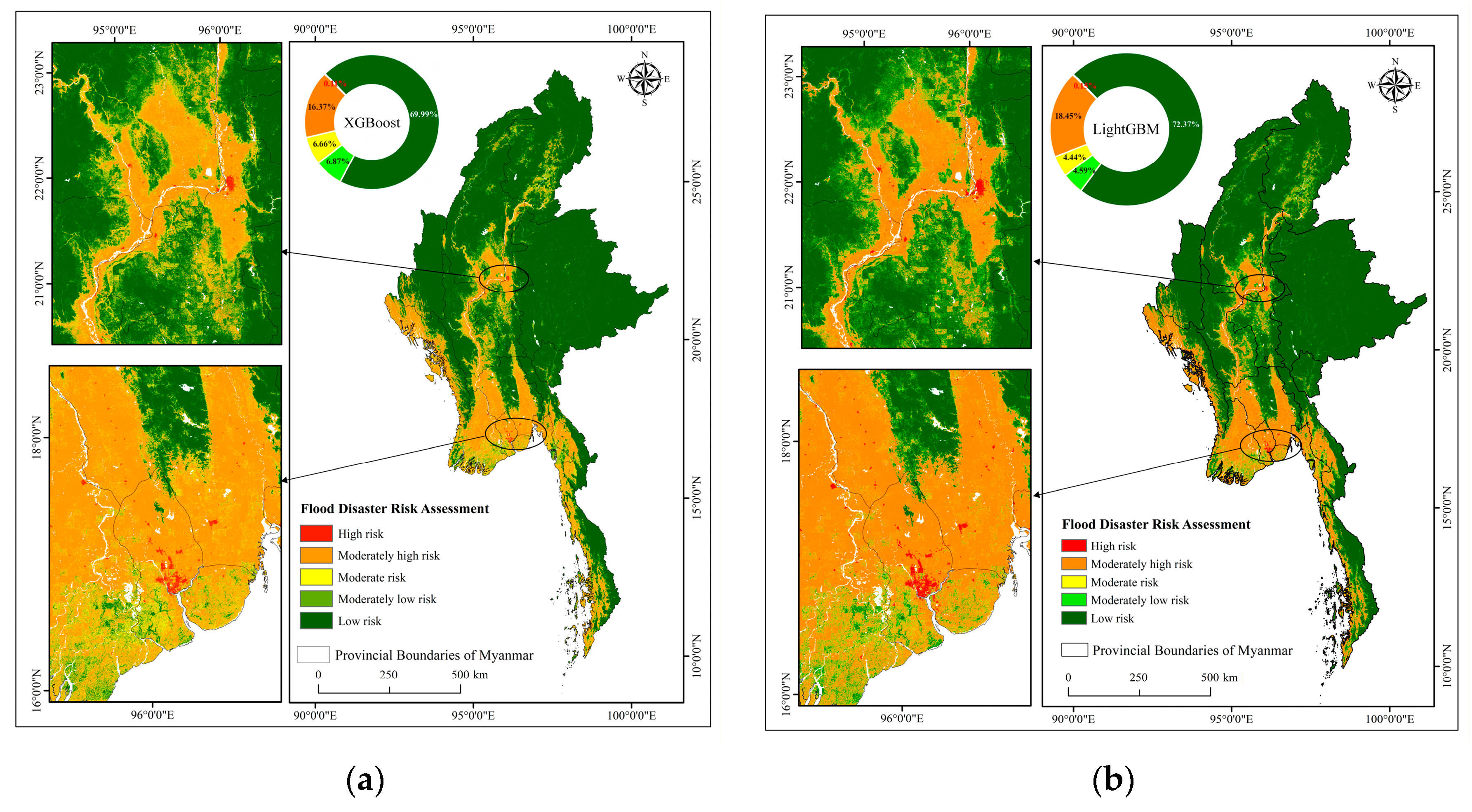
To comprehensively evaluate flood disaster risk, this study integrated the flood susceptibility indices derived from the XGBoost and LightGBM models with population and economic data to construct a “natural vulnerability-social exposure” risk matrix, aimed at identifying flood risk hotspots across Myanmar (Figure 14). According to the XGBoost results, approximately 0.11% of the study area is classified as high-risk, while 16.37% and 6.66% fall within the moderately high and moderate risk categories, respectively. In total, around 23.14% of the territory is exposed to relatively high flood risk. In addition, 6.87% of the area is categorized as moderately low risk, and 69.99% as low risk. The LightGBM model yields a comparable spatial distribution, predicting 0.15% of the area as high risk, 18.45% as moderately high risk, and 4.44% as moderate risk—a combined 23.04% of the country at relatively high flood risk levels. Meanwhile, 4.59% and 72.73% of the area are identified as moderately low and low risk, respectively. Although slight numerical differences exist between the two models, both exhibit high spatial consistency. The high-risk zones are primarily concentrated in the Mandalay region and its surrounding middle reaches of the Irrawaddy River, as well as in the low-lying areas of the Yangon Delta. These regions are characterized by flat terrain, dense population, and intensive economic activities, while the flood control and drainage infrastructure remains relatively weak. Consequently, they exhibit greater flood vulnerability and social exposure. Overall, the results highlight that areas with the combination of high hydrological susceptibility, dense human settlements, and insufficient adaptive capacity should be prioritized in flood risk mitigation and emergency management strategies.

4. Discussion

This study demonstrates how topographic, hydrological, and ecological factors jointly influence flood susceptibility within a satellite-driven, high-resolution assessment framework. Among the flood-related driving factors, terrain-related variables—particularly DEM and slope—play a fundamental role in controlling surface runoff convergence and drainage efficiency. Low-lying plains with limited drainage capacity are therefore more prone to flood accumulation, especially during periods of sustained or intense rainfall. Such terrain-controlled flood processes have been widely documented in flood susceptibility and hydrological studies, underscoring the dominant influence of elevation and slope on runoff concentration and flood generation [22]. Precipitation frequency emerges as the dominant hydrological driver in this study, reflecting the strong influence of monsoonal rainfall regimes on flood occurrence in Myanmar, which is consistent with previous findings that emphasize rainfall frequency and intensity as primary triggers of flooding in monsoon-affected regions [45]. Vegetation conditions, represented by NDVI, generally exhibit a negative association with flood susceptibility by enhancing soil infiltration and evapotranspiration under moderate hydrological conditions. However, the mitigating effect of vegetation is scale- and event-dependent. Existing studies indicate that under extreme rainfall events or at large catchment scales, flood generation is predominantly controlled by precipitation intensity and basin-scale hydrological processes, while the buffering capacity of vegetation becomes limited or secondary. This limitation has been widely discussed in recent reviews of nature-based flood mitigation, which emphasize that the effectiveness of vegetation-based interventions varies with event magnitude and catchment characteristics [46]. Such remotely sensed vegetation indices have been widely applied to characterize regional ecological conditions and their spatiotemporal evolution [47], supporting their suitability as ecological indicators in large-scale flood susceptibility assessment, particularly in data-scarce regions where long-term field observations are unavailable. Collectively, these results indicate that the adopted framework effectively translates satellite-observed environmental information into physically interpretable flood susceptibility patterns at the national scale.

Both XGBoost and LightGBM achieved strong predictive performance (AUC > 0.93), while exhibiting different sensitivities to specific environmental drivers. LightGBM showed greater responsiveness to precipitation frequency and NDVI, suggesting an enhanced ability to capture nonlinear interactions between rainfall variability and vegetation conditions. In contrast, XGBoost was more sensitive to terrain-related variables such as DEM, slope, and curvature, indicating its relative strength in representing topography-controlled flood processes. Such differences in model sensitivity are consistent with previous studies showing that advanced ensemble learning algorithms can capture heterogeneous and nonlinear responses of multi-source predictors under complex environmental conditions [48]. The consistently high performance of both models further reflects the advantages of integrating multi-source remote sensing datasets, which provide spatially detailed and internally consistent inputs for machine-learning-based flood susceptibility modeling. Overall, the results confirm that gradient-boosting-based ensemble methods exhibit strong generalization capability and spatial robustness when applied to observation-based flood susceptibility assessment across diverse topographic and climatic settings [49].

Beyond natural susceptibility, this study extends flood assessment toward an integrated risk perspective by incorporating socioeconomic exposure indicators. Satellite-derived population density and nighttime light intensity are used to represent the spatial distribution of human settlements and economic activity, enabling the construction of a coupled natural vulnerability–social exposure flood-risk framework. Because these indicators are obtained from remote sensing observations, they offer an objective and spatially explicit alternative to traditional census-based data, which are often incomplete or outdated in developing regions [46]. Similar integrative perspectives have been emphasized in recent studies that link environmental processes with socioeconomic dimensions to support regional risk assessment and sustainable development planning [47]. In addition, the application of SHAP enhances model interpretability by quantifying the contribution and direction of influence of individual predictors, thereby reducing the black-box uncertainty commonly associated with machine-learning approaches and improving the transparency of flood susceptibility mapping [48,49]. Together, these elements strengthen the analytical linkage between environmental processes and human exposure in large-scale flood risk assessment.

Despite these advances, several limitations remain. First, heterogeneity in the temporal resolution and spatial coverage of multi-source datasets may affect local-scale accuracy, although the proposed framework demonstrates robust performance at the national scale. In addition, algorithmic comparisons are limited to gradient boosting decision tree models (XGBoost and LightGBM), which were selected for their favorable balance between predictive performance and interpretability under data-scarce conditions. More complex modeling approaches, such as convolutional neural networks (CNNs) or long short-term memory networks (LSTMs), may be explored in future studies as denser spatiotemporal datasets and larger labeled samples become available. Second, the proposed framework does not explicitly simulate key physical hydrological and meteorological processes, including rainfall infiltration, runoff generation, flow concentration, and channel routing. Soil-related hydrological factors—such as spatial variability in infiltration capacity and antecedent moisture conditions—as well as event-scale precipitation characteristics (e.g., rainfall intensity, duration, and fine-scale spatial distribution), are not explicitly incorporated. Instead, these influences are indirectly represented through multi-source remote sensing indicators, including long-term precipitation statistics, terrain attributes, vegetation indices, and land-use information, which serve as proxies for their aggregated effects at a regional scale. The absence of explicit process representation may introduce uncertainty in characterizing flood volume and propagation behavior, particularly during extreme or short-duration rainfall events. Third, human activities are not modeled as dynamic physical processes in the current framework. Socioeconomic indicators such as population density and nighttime light intensity are primarily used to characterize spatial patterns of human exposure; however, their relatively short temporal coverage limits the representation of long-term flood risk trends driven by socioeconomic development. Moreover, detailed socioeconomic variables—such as industrial and agricultural planning and the spatial configuration of major infrastructure—are not explicitly included, and human-induced modifications to flood dynamics, including urbanization-driven land-cover changes and the blocking or diversion effects of roads and bridges, are not directly represented. Consequently, anthropogenic influences on flood routing and inundation processes may be underestimated. In addition, this study does not explicitly account for future climate change impacts, such as increased precipitation extremes or sea-level rise. Incorporating climate model projections (e.g., CMIP6) would enable the assessment of flood susceptibility and risk under different climate scenarios and enhance the applicability of the framework for long-term risk management.

Future research could address these limitations by developing hybrid frameworks that couple data-driven flood susceptibility models with distributed hydrological or hydrodynamic models (e.g., SWAT, VIC, or HEC-HMS), enabling more explicit representation of runoff generation, flow routing, and human-induced hydraulic modifications. Furthermore, integrating high-temporal-resolution precipitation data, satellite-derived soil moisture products, long-term socioeconomic datasets, climate projections, and information on urban expansion would support integrated flood risk assessment frameworks that explicitly link natural susceptibility and socioeconomic exposure. Such advances would also facilitate the development of comprehensive technological systems combining multi-source satellite remote sensing, ground-based IoT observations, and intelligent analytics for flood monitoring, early warning, assessment, and emergency response.

5. Conclusions

This study develops and applies a nationwide, high-resolution framework for flood susceptibility and integrated risk assessment in Myanmar by leveraging multi-source remote sensing data and ensemble machine-learning algorithms on the Google Earth Engine platform. Rather than focusing solely on identifying flood-prone areas, this framework emphasizes a transferable and interpretable assessment workflow suitable for data-scarce regions, enabling reproducible flood-risk mapping primarily based on satellite observations. The application of this framework demonstrates its effectiveness in capturing flood-prone environments while achieving excellent predictive performance (AUC > 0.93) across two independent ensemble models. Precipitation frequency, DEM, and NDVI are identified as the key driving factors influencing flood susceptibility, reflecting the capability of satellite-derived indicators to characterize hydrometeorological variability, terrain conditions, and vegetation dynamics at high spatial resolution. The strong spatial consistency between XGBoost and LightGBM further confirms the robustness of the assessment results under complex topographic and climatic conditions.

Building on the flood susceptibility analysis, this study integrates satellite-derived population density and nighttime light data to construct a coupled natural vulnerability–social exposure flood-risk framework. The resulting risk maps highlight the value of remotely observed socioeconomic indicators in linking environmental hazards with human exposure, thereby supporting flood-risk-informed spatial planning and disaster mitigation in monsoon-affected regions.

Methodologically, this study demonstrates the systematic integration of multi-source remote sensing observations, ensemble learning algorithms, and SHAP-based interpretability analysis within a unified GEE-based workflow. The main contributions lie in the coordinated use of high-resolution, multi-temporal remote sensing indicators, explainable machine-learning techniques, and scalable cloud-based processing for large-scale flood susceptibility and risk assessment in data-scarce monsoon regions. Overall, this study provides a practical and transferable technical pathway for flood susceptibility and risk analysis, contributing to proactive flood-risk governance, climate resilience, and sustainable disaster prevention planning in Myanmar and similar environments.

References

1. Zhang, S. Flood disaster prediction and risk assessment based on data analysis and machine learning. Inf. Technol. Informatiz. 2024, 8, 189–194. [Google Scholar] [CrossRef]
2. United Nations Office for Disaster Risk Reduction (UNDRR); Centre for Research on the Epidemiology of Disasters (CRED). The Human Cost of Disasters: An Overview of the Last 20 Years (2000–2019); United Nations Office for Disaster Risk Reduction: Geneva, Switzerland, 2020; Available online: https://www.undrr.org/publication/human-cost-disasters-overview-last-20-years-2000–2019 (accessed on 6 November 2025).
3. Wei, X.K. Study on Runoff Variation Prediction Based on Multiple Deep Learning Methods. Ph.D. Dissertation, Nanjing University of Information Science and Technology, Nanjing, China, 2024. [Google Scholar] [CrossRef]
4. Akbarian, H.; Gheibi, M.; Hajiaghaei Keshteli, M.; Rahmani, M. A hybrid novel framework for flood disaster risk control in developing countries based on smart prediction systems and prioritized scenarios. J. Environ. Manag. 2022, 312, 114939. [Google Scholar] [CrossRef] [PubMed]
5. World Bank. Myanmar Floods and Landslides: Post Disaster Needs Assessment; World Bank: Washington, DC, USA, 2016; Available online: https://www.worldbank.org/en/country/myanmar/publication/myanmar-floods-and-landslides-post-disaster-needs-assessment (accessed on 6 November 2025).
6. Varra, G.; Della Morte, R.; Tartaglia, M.; Fiduccia, A.; Zammuto, A.; Agostino, I.; Booth, C.A.; Quinn, N.; Lamond, J.E.; Cozzolino, L. Flood susceptibility assessment for improving the resilience capacity of railway infrastructure networks. Water 2024, 16, 2592. [Google Scholar] [CrossRef]
7. Edamo, M.L.; Ukumo, T.Y.; Lohani, T.K.; Dile, Y.T.; Tefera, Z.M. A comparative assessment of multi-criteria decision-making analysis and machine learning methods for flood susceptibility mapping and socio-economic impacts on flood risk in the Abela–Abaya floodplain of Ethiopia. Environ. Chall. 2022, 9, 100629. [Google Scholar] [CrossRef]
8. Khaldi, L.; Elabed, A.; El Khanchoufi, A. Multidimensional risk assessment based on flood susceptibility mapping and multiple socioeconomic variables under climate change. Sci. Afr. 2025, 28, e02834. [Google Scholar] [CrossRef]
9. Mandal, A.K.; Thapa Chhetri, M.; Bloetscher, F.; Yong, Y.; Su, H. Semi-automated workflow for multi-basin, multi-scenario flood risk modeling, mapping, and impact assessment. Nat. Hazards 2025, 121, 14425–14441. [Google Scholar] [CrossRef]
10. Jayawardane, P.; Rajapakse, L.; Siriwardana, C. Integrated flood risk management for urban resilience: A multi-method framework combining hazard mapping, hydrodynamic modelling, and economic impact assessment. Resilient Cities Struct. 2025, 4, 117–131. [Google Scholar] [CrossRef]
11. Agrawal, R.; Singh, S.K.; Kanga, S.; Sajan, B.; Meraj, G.; Kumar, P. Advancing flood risk assessment through integrated hazard mapping: A Google Earth Engine-based approach for comprehensive scientific analysis and decision support. J. Clim. Change 2024, 10, 47–60. [Google Scholar] [CrossRef]
12. Sibandze, P.; Kalumba, A.M.; Aljaddani, A.H.; Zhou, L.; Afuye, G.A. Geospatial mapping and meteorological flood risk assessment: A global research trend analysis. Environ. Manag. 2025, 75, 137–154. [Google Scholar] [CrossRef]
13. Seeger, K.; Minderhoud, P.S.J.; Peffeköver, A.; Vogel, A.; Brückner, H.; Kraas, F.; Oo, N.W.; Brill, D. Assessing land elevation in the Ayeyarwady Delta (Myanmar) and its relevance for studying sea level rise and delta flooding. Hydrol. Earth Syst. Sci. 2023, 27, 2257–2281. [Google Scholar] [CrossRef]
14. Yin, K.; He, L.; Liu, S.; Xu, S. Effects of climate change on the estimation of extreme sea levels in the Ayeyarwady Sea of Myanmar by Monte Carlo simulation. Water 2025, 17, 429. [Google Scholar] [CrossRef]
15. Latt, Z.Z.; Wittenberg, H. Hydrology and flood probability of the monsoon-dominated Chindwin River in northern Myanmar. J. Water Clim. Change 2015, 6, 144–160. [Google Scholar] [CrossRef]
16. Vogel, A.; Seeger, K.; Brill, D.; Brückner, H.; Kyaw, A.; Myint, Z.N.; Kraas, F. Towards integrated flood management: Vulnerability and flood risk in the Ayeyarwady Delta of Myanmar. Int. J. Disaster Risk Reduct. 2024, 114, 104723. [Google Scholar] [CrossRef]
17. Kalita, N.; Bhattacharjee, N.; Sarmah, N.; Nath, M.J. Estimation of flood hazard zones of Noa River Basin using maximum entropy model in GIS. Nat. Environ. Pollut. Technol. 2025, 24, B4216. [Google Scholar] [CrossRef]
18. Smith, A.; Bates, P.D.; Wing, O.; Sampson, C.; Quinn, N.; Neal, J. New estimates of flood exposure in developing countries using high-resolution population data. Nat. Commun. 2019, 10, 1814. [Google Scholar] [CrossRef] [PubMed]
19. Wang, Y.; Liu, K. Measurement of urban spatial structure and its influencing factors in China based on nighttime light data. Geogr. Geo-Inf. Sci. 2025, 41, 47–55. (In Chinese) [Google Scholar] [CrossRef]
20. Lehner, B.; Grill, G. Global river hydrography and network routing: Baseline data and new approaches to study the world’s large river systems. Hydrol. Process. 2013, 27, 2171–2186. [Google Scholar] [CrossRef]
21. Natarajan, L.; Usha, T.; Gowrappan, M.; Kasthuri, B.P.; Moorthy, P.; Chokkalingam, L. Flood susceptibility analysis in Chennai Corporation using frequency ratio model. J. Indian Soc. Remote Sens. 2021, 49, 1533–1543. [Google Scholar] [CrossRef]
22. AlJuaidi, A.E.M. The interaction of topographic slope with various geo-environmental flood-causing factors on flood prediction and susceptibility mapping. Environ. Sci. Pollut. Res. Int. 2023, 30, 59327–59348. [Google Scholar] [CrossRef]
23. Tang, Y.; Xi, S.; Chen, X.; Lian, Y. Quantification of multiple climate change and human activity impact factors on flood regimes in the Pearl River Delta of China. Adv. Meteorol. 2016, 2016, 3928920. [Google Scholar] [CrossRef]
24. Huang, M.; Zhong, S.; Ge, Y.; Lin, H.; Chang, L.; Zhu, D.; Zhang, L.; Xiao, C.; Altan, O. Evaluating the Performance of SDGSAT-1 GLI Data in Urban Built-Up Area Extraction from the Perspective of Urban Morphology and City Scale: A Case Study of 15 Cities in China. IEEE J. Sel. Top. Appl. Earth Obs. Remote Sens. 2025, 18, 17166–17180. [Google Scholar] [CrossRef]
25. Song, S.B.; Kang, Y.; Song, X.Y.; Wang, X.J.; Jin, J.L. Principles and Applications of Univariate Hydrological Series Frequency Calculation; Science Press: Beijing, China, 2018; pp. 631–652. (In Chinese) [Google Scholar]
26. Yang, J.; Wan, Z.; Borjigin, S.; Zhang, D.; Yan, Y.; Chen, Y.; Gu, R.; Gao, Q. Changing trends of NDVI and their responses to climatic variation in different types of grassland in Inner Mongolia from 1982 to 2011. Sustainability 2019, 11, 3256. [Google Scholar] [CrossRef]
27. Qu, L.; Huang, Y.; Yang, L.; Li, Y. Vegetation restoration in response to climatic and anthropogenic changes in the Loess Plateau, China. Chin. Geogr. Sci. 2020, 30, 89–100. [Google Scholar] [CrossRef]
28. Gong, Z.N.; Zhao, S.Y.; Gu, J.Z. Correlation analysis between vegetation coverage and climate drought conditions in North China during 2001–2013. J. Geogr. Sci. 2017, 27, 143–160. [Google Scholar] [CrossRef]
29. Chan, J.Y.L.; Leow, S.M.H.; Bea, K.T.; Cheng, W.K.; Phoong, S.W.; Hong, Z.-W.; Chen, Y.-L. Mitigating the Multicollinearity Problem and Its Machine Learning Approach: A Review. Mathematics 2022, 10, 1283. [Google Scholar] [CrossRef]
30. Kalnins, A.; Praitis Hill, K. Additional Caution Regarding Rules of Thumb for Variance Inflation Factors: Extending O’Brien to the Context of Specification Error. Qual. Quant. 2024, 59, 1–24. [Google Scholar] [CrossRef]
31. Szczepanek, R. Daily streamflow forecasting in mountainous catchment using XGBoost, LightGBM and CatBoost. Hydrology 2022, 9, 226. [Google Scholar] [CrossRef]
32. Sanders, W.; Li, D.F.; Li, W.Z.; Fang, Z.N. Data-driven flood alert system (FAS) using extreme gradient boosting (XGBoost) to forecast flood stages. Water 2022, 14, 747. [Google Scholar] [CrossRef]
33. Subbarayan, S.; Devanantham, A.; Nagireddy Masthan, R.; Parthasarathy, K.S.S.; Janardhanam, N.; Subbarayan, S.; Vivek, S. Flood susceptibility mapping using machine learning boosting algorithms techniques in Idukki District of Kerala, India. Urban. Clim. 2023, 49, 101503. [Google Scholar] [CrossRef]
34. Abu El Magd, S.A.; Pradhan, B.; Alamri, A. Machine learning algorithm for flash flood prediction mapping in Wadi El-Laqeita and surroundings, Central Eastern Desert, Egypt. Arab. J. Geosci. 2021, 14, 323. [Google Scholar] [CrossRef]
35. Ke, G.; Meng, Q.; Finley, T.; Wang, T.; Chen, W.; Ma, W.; Ye, Q.; Liu, T.-Y. LightGBM: A Highly Efficient Gradient Boosting Decision Tree. In Proceedings of the 31st International Conference on Neural Information Processing Systems (NeurIPS 2017), Long Beach, CA, USA, 4–9 December 2017; pp. 3149–3157. [Google Scholar]
36. Xu, K.; Han, Z.T.; Xu, H.S.; Bin, L.L. Rapid prediction model for urban floods based on a light gradient boosting machine approach and hydrological–hydraulic model. Int. J. Disaster Risk Sci. 2023, 14, 79–97. [Google Scholar] [CrossRef]
37. Osei Kyei, R.; Ampratwum, G.; Komac, U.; Narbaev, T. Critical analysis of the emerging flood disaster resilience assessment indicators. Int. J. Disaster Resil. Built Environ. 2025, 16, 417–436. [Google Scholar] [CrossRef]
38. Zou, Y.; Wang, X.R. Analysis of influencing factors of terrestrial carbon sinks in China based on LightGBM model and Bayesian optimization algorithm. Sustainability 2025, 17, 4836. [Google Scholar] [CrossRef]
39. Kiani, A.; Motamedvaziri, B.; Khaleghi, M.R.; Ahmadi, H. Spatial prediction of flood susceptible areas using machine learning methods in the Siahkhor Watershed of Kermanshah Province. Earth Sci. Inform. 2024, 18, 20. [Google Scholar] [CrossRef]
40. Krasnodębska, K.; Goch, W.; Uhl, J.H.; Verstegen, J.A.; Pesaresi, M. Advancing precision, recall, F-score, and Jaccard index: An approach for continuous, ratio-scale measurements. Environ. Model. Softw. 2025, 193, 106614. [Google Scholar] [CrossRef]
41. Luque, A.; Carrasco, A.; Martín, A.; de las Heras, A. The impact of class imbalance in classification performance metrics based on the binary confusion matrix. Pattern Recognit. 2019, 91, 216–231. [Google Scholar] [CrossRef]
42. Pradhan, B.; Lee, S.; Dikshit, A.; Kim, H. Spatial flood susceptibility mapping using an explainable artificial intelligence (XAI) model. Geosci. Front. 2023, 14, 101625. [Google Scholar] [CrossRef]
43. Lundberg, S.M.; Erion, G.; Chen, H.; DeGrave, A.; Prutkin, J.M.; Nair, B.; Katz, R.; Himmelfarb, J.; Bansal, N.; Lee, S.-I. From local explanations to global understanding with explainable AI for trees. Nat. Mach. Intell. 2020, 2, 56–67. [Google Scholar] [CrossRef]
44. Omar, S.; Ayzel, G.; de Souza, A.C.T.; Bronstert, A.; Heistermann, M. Towards urban flood susceptibility mapping using data-driven models in Berlin, Germany. Geomatics, Nat. Hazards Risk 2022, 13, 1640–1662. [Google Scholar] [CrossRef]
45. Liu, L.Y.; Li, H.E.; Zhou, N.; Wang, X.B.; Wang, F.; Zhang, Z. Study on characteristics, mechanisms, and adaptive countermeasures of catastrophic dam-break disasters under climate change. J. Hydraul. Waterw. Eng. 2025, 5, 14–28. (In Chinese) [Google Scholar]
46. Herath, P.; Prinsley, R.; Croke, B.; Vaze, J.; Pollino, C. A bibliometric analysis and overview of the effectiveness of Nature-based Solutions in catchment scale flood mitigation. Nat.-Based Solut. 2025, 7, 100235. [Google Scholar] [CrossRef]
47. Sun, H.; Huang, M.; Lin, H.; Ge, Y.; Zhu, D.; Gong, D.; Altan, O. Spatiotemporal Dynamics of Ecological Environment Quality in Arid and Sandy Regions with a Particular Remote Sensing Ecological Index: A Study of the Beijing-Tianjin Sand Source Region. Geo-Spat. Inf. Sci. 2025, 1–20. [Google Scholar] [CrossRef]
48. Hussain, M.A.; Chen, Z.; Pradhan, B.; Meena, S.R.; Zhou, Y. Hybrid heterogeneous ensemble learning framework for flood susceptibility mapping in Balochistan, Pakistan. J. Hydrol. Reg. Stud. 2025, 61, 102718. [Google Scholar] [CrossRef]
49. Xu, J.; Ren, Y.; Zhang, H.; Fu, S. Research on Flood Occurrence Prediction Based on Entropy Weighted TOPSIS and Ensemble Machine Learning. In Proceedings of the 2024 8th International Workshop on Materials Engineering and Computer Sciences (IWMECS); Francis Academic Press: London, UK, 2024; pp. 45–51. [Google Scholar] [CrossRef]
Figure 1. Geographic location and elevation distribution of the study area. (a) Location of Myanmar within Southeast Asia; (b) Digital Elevation Model (DEM) of Southeast Asia, providing regional topographic context; (c) DEM of Myanmar, representing the study area used for flood susceptibility and risk assessment.
Ijgi 15 00045 g001
Figure 2. Spatial distribution maps of flood-related influencing factors in Myanmar. (a) DEM (m), (b) slope (°), (c) aspect (°); flat areas with zero slope are assigned a value of −1, (d) curvature (dimensionless), (e) annual precipitation frequency (dimensionless), (f) TWI, (g) SPI (dimensionless), (h) distance to rivers (classes), (i) river density (km·km−2), (j) NDVI (dimensionless), (k) land-use type, (l) population density (persons·km−2), and (m) nighttime light intensity (nW·cm−2·sr−1).
Ijgi 15 00045 g002aIjgi 15 00045 g002bIjgi 15 00045 g002c
Figure 3. UNOSAT-derived flood extent maps for Myanmar during 2020–2024, showing the spatial distribution of satellite-observed flood inundation used for flood sample extraction and independent validation.
Ijgi 15 00045 g003
Figure 4. Technical workflow of flood-susceptibility and risk assessment in Myanmar.
Ijgi 15 00045 g004
Figure 5. Correlation matrices of influencing factors: (a) Overall correlation matrix of influencing factors; (b) Filtered correlation matrix after removing highly correlated variables (threshold = 0.75).
Ijgi 15 00045 g005
Figure 6. Model evaluation metrics.
Ijgi 15 00045 g006
Figure 7. Confusion matrices of the two ensemble learning models: (a) XGBoost confusion matrix; (b) LightGBM confusion matrix.
Ijgi 15 00045 g007
Figure 8. Area under the receiver operating characteristic (ROC) curves of ensemble models: (a) XGBoost ROC curves by individual factor; (b) LightGBM ROC curves by individual factor.
Ijgi 15 00045 g008
Figure 9. Feature importance evaluation of ensemble learning models: (a) XGBoost feature importance ranking; (b) LightGBM feature importance ranking.
Ijgi 15 00045 g009
Figure 10. SHAP-based feature importance analysis of ensemble learning models: (a) XGBoost SHAP feature importance; (b) LightGBM SHAP feature importance.
Ijgi 15 00045 g010
Figure 11. SHAP-based interpretation of single-sample flood susceptibility prediction: (a) XGBoost model; (b) LightGBM model.Red and blue bars represent positive and negative contributions of individual features to the model prediction, respectively.
Ijgi 15 00045 g011
Figure 12. Comparison of Feature Importance between XGBoost and LightGBM Models.
Ijgi 15 00045 g012
Figure 13. Flood susceptibility mapping results: (a) XGBoost model; (b) LightGBM model.
Ijgi 15 00045 g013
Figure 14. Flood disaster risk assessment maps: (a) XGBoost model risk assessment; (b) LightGBM model risk assessment.
Ijgi 15 00045 g014