Statistical Depth Measures in Density-Based Clustering with Automatic Adjustment for Skewed Data

Abstract

Statistical data depth measures have been applied to density-based clustering techniques in an effort to achieve robustness in parameter selection via the affine invariant property of the depth measure. Specifically, the Mahalanobis depth measure is used in the application of DBSCAN. In this paper, we examine properties of the Mahalanobis depth measure that lead to instances where it fails to detect clusters in DBSCAN, whereas Euclidean distance is able to differentiate the clusters. We propose two solutions to the problems induced by these properties. The first re-examines clusters to determine if data shape is causing multiple clusters to be grouped into a single cluster. The second examines the use of a different measure as an alternate depth function. Experiments are provided.

1. Introduction

Cluster analysis seeks to extract information from data by grouping data points together based on some notion of similarity. Applications of clustering are widely used, including in image recognition, trajectory analysis, genetic sequencing, morphology analysis, etc.

Statistical data depth measures are measures that, traditionally, provide a value of outlyingness of a data point with respect to a data set. The term depth is used because it is common to construct values such that a point with a larger depth value is interpreted as deeper within the data set (i.e., more central with respect to some notion of centrality) and a lower value as shallower, or more outlying.

Density-based clustering algorithms, such as DBSCAN [1] are a popular choice for clustering data. An advantage of density-based algorithms is that they have the ability to identify clusters regardless of the shape of cluster, they have the ability to identify clusters that are not necessarily linear separable, and they are robust with respect to some levels of noise. DBSCAN is often implemented using Euclidean distance between data points to determine density. A brief review of DBSCAN is provided in Section 4.1.

Recent work has looked into the use of data depth measures to compute distance values between points as a way to determine density in density-based clustering algorithms, particularly DBSCAN [2,3]. Generally, a data depth measure is used in place of Euclidean distance to determine the relative distance between data points in order to compute density. Because data depth measures are typically defined as a measure of a single point with respect to a point set, data depth measures are altered to compute the relative depth of two points with respect the distribution of a point set (Section 3). The advantage of using data depth measures instead of distance is that, depending on the depth measure used, data depth measures provide affine invariance; thus, applications in which data scale may be different (e.g., images taken from drones at varying altitudes) may be clustered using similar parameters as input to the clustering algorithm, whereas distance parameters must be adjusted according to data scale when using the Euclidean distance measure. Recent work studies Mahalanobis Depth (MD) (based on Mahalanobis distance [4]) (Section 3.1), in particular, as a depth measure in clustering.

In this paper, we explore properties of the MD measure and their effect on the application of MD to clustering. Furthermore, we develop a second depth measure based on a measure known as Projection Depth (PD) [5,6,7]. The contributions of this paper are as follows: (1) identify two properties of MD that affect its ability to identify density-based clusters in some situations, (2) develop examples to illustrate such cases, (3) introduce a novel, MD-based clustering algorithm that can overcome one of the identified limitations, and (4) develop a depth measure for clustering applications based on projection depth that maintains some desirable properties of MD but can overcome the other identified limitation.

The remainder of the paper is structured as follows: Section 2 reviews related literature; Section 3 defines desirable properties of depth functions, develops the MD measure, and develops the PD measure; Section 4 reviews the DBSCAN algorithm, shows how to use it with depth measures, and develops an algorithm to overcome a discovered limitation of the DBSCAN algorithm paired with the MD measure; experiments are presented in Section 5; finally, in Section 6, we draw some conclusions.

2. Related Work

Research into clustering, in general, is mature. In this paper, we restrict our focus to density-based clustering and clustering with data depth.

K-means clustering algorithms focus on computing clusters by minimizing a distance measure of points in clusters to K centroids where K is chosen in advance [8,9]. Traditional K-means approaches use Euclidean distance to measure distances from points to centers, which performs well when clusters are spherical. The use of MD as a distance measure allows one to improve K-means performance when clusters are elliptical [10,11].

More recently, investigations into using depth measures as distance measures in density-based clustering have been proposed. Data Depth Based Clustering Algorithm (DBCA) [2] proposes the use of the MD measure as the distance measure in a DBSCAN-like algorithm. Interestingly, the presentation of the algorithm does not use a parameter to indicate the minimum size of a cluster, essentially hard-coding a default minimum cluster size to 2. It is a minor change to add the parameter, but by choosing the value as static, one can make use of implementation tricks to result in a faster running time for the algorithm (although the theoretical running time remains the same).

In [3], MD is again used in a DBSCAN-like setting, as well as a different clustering approach, named CRAD, in which a histogram is computed for each point in a data set such that each bin in the histogram shows the number of points that fall within a ellipsoidal segment of space centered at the point (i.e., a histogram of point densities for each point). Clusters are then determined based on changes in density in those histograms. While CRAD is a different style of clustering algorithm, we consider it here since it is density-based and does use MD. CRAD performs well, but has some properties that can cause poor results in certain situations (particular with respect to the presence of noise) (Section 5).

MD is but one of a variety of data depth measures (see [12,13] for treatments of various measures). In this paper, we focus on two depth measures: MD and PD. We focus on MD since it is already proposed in clustering, and we identify two properties of MD that may lead to poor clustering results in certain situations when using density-based clustering. We also investigate the use of PD with density-based clustering, which does not suffer from the same properties as MD, but which trades this for less resilience for data under shearing transformations.

3. Statistical Depth Functions

In general, a depth function $D(x,P)$ for a data set $P\subseteq {\mathbb{R}}^d$ provides a center-outward ordering of the points in P with respect to P. One useful applications of such functions is the determination of outliers since, depending on the depth function, outlyingness can be defined based on depth values of individual points with respect to the underlying point set. A thorough treatment of depth functions and their properties is found in [12].

The notion of depth functions describes a class of functions, but for the purposes of clustering, functions with certain desirable properties receive the most interest. Those properties are: (1) affine invariance, (2) maximality at the center, (3) monotonicity relative to the deepest point, and (4) vanishing at infinity. These properties allow a depth function to perform robustly in applications useful for clustering since the underlying coordinate system or scale of measurements of a distribution will not affect the depth calculations of points, and depth measurements change monotonically as points lie further away from the center of a data set.

In this paper, we will investigate two depth functions: Mahalanobis Depth (MD) satisfies the properties above; and Projection Depth (PD) satisfies the last 3 properties, maintains invariance under translation, rotation, and scaling such that the scale is identical on all axes, but is sensitive to shearing.

3.1. Mahalanobis Depth

Let M positive definite $d\times d$ matrix defining an elipsoid estimating the shape of a point distribution in d-dimensional space. MD is based on the notion of a distance value between two points in ${\mathbb{R}}^d$ with respect M; in other words, the distance between two such points is scaled with respect to M. The MD with respect to M, denoted $d_M$, is then:

$$d_M(x,y)={(x-y)}^T{M}^{-1}(x-y)$$

(1)

If we choose y as the ‘center’ point of a point set X with distribution F, we achieve a distance value from the center to a point. A typical choice for M is the covariance matrix of X, denoted K, and a typical choice for the center is the mean of X, denoted $\mu \left(X\right)$:

$$d_K(x;F)={(x-\mu \left(X\right))}^T{K}^{-1}(x-\mu \left(X\right))$$

(2)

For the purposes of clustering, we require the distance between two arbitrary points in a set, so we modify Equation (2):

$$d_K(x,y\in X)={(x-y)}^T{K}^{-1}(x-y)$$

(3)

where $x,y\in X$ and K is the covariance matrix of X.

As stated, the function is a distance measure, rather than a depth measure, since outlyingness is calculated as larger values. Although a distance measure may be used directly for clustering an alternate form is to convert the distance to a depth measure between 0 and 1 where points with large distance will have depth lower depth and points with close distance will have larger depth. The term depth arises from the form of the measure where a point is measured in relation to a centroid, such that points with higher depth are deeper within the data set. We convert the distance measure to a depth function:

$$D_M(x,y\in X)={(1+d_K(x,y))}^{-1}$$

(4)

where K is the covariance matrix of X. Because the covariance matrix is used, the depth between two points reflects the Euclidean distance scaled along the eigenvectors of the covariance matrix defined by the point set, which correspond to the directions of maximum variance in the point set.

One drawback to the MD equation as provided is that it is based on the mean of the data set, which can be poorly affected in the presence of outliers. To combat this, one may use robust covariance estimators which rely on sampling to minimize the effect of outliers on the mean [14,15,16]. For the experiments in this paper, we use the mean of the data set.

3.2. Interpretation of Mahalanobis Depth

This section provides an intuitive description of Mahalanobis Depth and its properties using examples and observations which will motivate the need for our proposed algorithm described in Section 4. In short, given a point set P, the distance Mahanalobis distance between two points in P is Euclidean distance between the points scaled by the information contained in the covariance matrix for P.

Equation (2) provides a depth function that indicates the normalized distance of a query point with respect to the center of a distribution of points based on the covariance matrix defined by the points. Because the depth of the query point is based on the covariance matrix of the underlying points, the depth is scaled based on the variance of the underlying data. For example, consider a distribution of 2-dimensional points P centered on the origin such that $\forall p=(x,y)\in P:x\in [-10,10],y\in [-2,2]$. The covariance matrix for P will indicate much larger variance along the x axis than the y axis; thus, the computed value for $p_1=(2,0)$ will be higher than the computed value for $p_2=(0,2)$. In other words, a unit of computed depth along the x axis will cover more Euclidean distance than an equivalent unit of computed depth along the y axis for points in P. Similarly, this behavior holds when using Equation (3) to judge the distance of two points relative to each other with respect to covariance of the underlying distribution of points, leading to the following observations:

Observation 1.

The depth value calculated over a data set of points P using Equation (2) or Equation (3) effectively provides a value that is scaled to remove the variance along the eigenvectors of the covariance matrix defined over P.

Observation 1 is precisely why the use of MD in K-means clustering produces better results than Euclidean distance for ellipsoidal shaped clusters. However, it also has implications that may not be desirable when the range of data naturally occurs along dimensions of differing variance, despite the clusters themselves not having highly differing variance among the dimensions. Which leads to a second observation:

Observation 2.

The representative ellipse of a data set of points P (as defined by the eigenvectors of the covariance matrix of P scaled by their eigenvalues) defines scaling of depth values when using MD, which may have implications for detecting local clusters whose representative ellipses have different orientation and shape than the global representative ellipse.

Observation 2 indicates that the scale of the overall distribution of points defines the Euclidean distances covered by a unit of depth in some direction for a set of points P. In clustering, this can have implications that prevent discovery of clusters in some applications when the scales of data along the eigenvectors of the covariance matrix differ greatly. For example, Figure 1 depicts data points that fall into two clusters, but that have significantly more variance in the x direction than the y direction. Since the MD value of two points is scaled by the covariance matrix of the data, one unit of MD in the x direction will correspond to a greater Euclidean distance than a unit of MD in the y direction. Because the two clusters in Figure 1 are defined by a separation in the x direction, that separation must be large enough to overcome the scaling differences of the data along the eigenvectors of the covariance matrix (the axes in this case) in order for the clusters to be detected. Indeed, in this example, 1 unit of Euclidean distance along the x axis corresponds to a depth value of $0.973$ and 1 unit of Euclidean distance along the y axis corresponds to a depth value of $0.425$; thus, once a depth value is reached that can distinguish the gap between the clusters in the x direction, the points within the two clusters are too far apart in the y direction to be clustered together. Therefore, the data set shown in Figure 1 cannot be clustered correctly when using a DBSCAN algorithm with the MD metric as is done in DBCA. We denote such cases as having high-dimensional skew.

In later sections, we provide techniques to deal with high-dimensional skew. For now we note that such skew may result due to the domain of the data. For example, a data set containing trajectories of vehicles that travel from New York to Chicago will naturally have greater range in one dimension than another. Similarly, location data taken on a peninsula or island may be geographically constrained to an area that is much longer in one dimension than another.

3.3. Projection Depth

The notion of projection depth is to define the depth of a point in a point set based on its distance with respect to the median of the point set in a 1-dimensional projection. We begin by defining projection distance, and later convert to a depth function. Specifically, the projection distance of an individual point should be maximal:

$$D(x\in X)=\underset{\Vert u\Vert =1}{sup}{\displaystyle \frac{|u^{T}x-\mathrm{Med}\left(u^{T}X\right)|}{\mathrm{MAD}\left(u^{T}X\right)}}$$

(5)

where X is a point set, $\Vert ·\Vert$ is the Euclidean norm, u is a unit vector to project point values to a single dimension, $Med$ is the median of values of points projected by the unit vector, and $MAD$ is the median absolute deviation for a set Y such that $MAD\left(Y\right)=Med\left(\right|Y-Med\left(Y\right)\left|\right)$ (in other words, the median absolute deviation from the median value of points projected by the unit vector).

Clearly, the above equation is suited to querying a point set for the distance of an individual point, but is less useful for comparing the depths of points since two points may have depths that depend on different unit vectors to achieve maximality, which limits usefulness in clustering applications. Therefore, we modify Equation (5) to use a single unit vector for all points in the point set to allow the direct pairwise comparison of projection distance of points. In order to achieve a notion of maximality, we choose the unit vector to be the vector along which the maximum variance of the data set lies. Thus, for data set X, we choose the vector u to be eigenvector corresponding to the largest eigenvalue of the covariance matrix of X (the 1st principal component of X); therefore, with u defined as such:

$$D(x\in X)={\displaystyle \frac{|u^{T}x-\mathrm{Med}\left(u^{T}X\right)|}{\mathrm{MAD}\left(u^{T}X\right)}}$$

(6)

Equation (6) provides the projection distance of a point relative to a point set such that we can meaningfully compare the projection distance of two points with respect to a single projection. The downside of this is clearly that we are using a 1-dimensional projection regardless of the original dimensionality of the data, and thus lose information (points that may be very far apart in some dimensions may have the same projection distance relative to the point set).

We make the observation that the idea of projection distance is to provide a distance value of a point that is scaled based on the ‘center’ of the distribution in some direction and the median absolute deviation in that direction. Intuitively, the eigenvector corresponding to the largest eigenvalue of the covariance matrix of a point set X corresponds to the first principal component of X in principle component analysis. Vectors along the principle components (scaled by the associated eigenvalues) effectively define the axes of a representative ellipse around X; thus, a sphere with radius of the magnitude of the first principle component defines a representative sphere for X. Thus, PD defined as such is related to MD, but can still correctly identify the clusters in Figure 1, since a unit of Euclidean distance covers the same amount of depth in any direction regardless of the relative variances of the principal components of a data set. Thus, domain knowledge of an application indicates when one depth measure is more appropriate than the other.

To achieve a meaningful projection distance, we adjust Equation (6) to report the projection distance between two points as the Euclidean distance between two points scaled by the $MAD$ of the point set when projected to the direction of the first principle component of the set. Let X be a point set and u be the eigenvector corresponding to the largest eigenvalue of covariance matrix of X:

$$D_{pdist}(x,y\in X)={\displaystyle \frac{|\Vert x-y\Vert -\mathrm{Med}(u^{T}X\left)\right|}{\mathrm{MAD}\left(u^{T}X\right)}}$$

(7)

Equation (7) yields a robust distance metric, but is not a depth value since it grows as points are further away from each other rather than shrink. We convert the distance measure to a depth measure as follows:

$$D_p(x,y)={(1+D_{pdist}(x,y))}^{-1}$$

(8)

We note that MD is considered affine invariant. PD is invariant with regards to some affine transformations, but shearing transformations can affect change the first principal component of a data set, relative to the original data set; since MD uses all principal components in scaling depth, it is more robust under shear. We investigate these properties in experiments.

Recall that MD suffers in cases of high-dimensional skew. PD does not have this property, and when in used in a DBSCAN-like algorithm, does successfully identify the clusters in Figure 1, where the use of MD did not. Thus, PD may be a better choice in the geographic examples mentioned previously or if some properties of the data are known to the user.

4. Algorithms

In this paper, we consider density-based clustering in the style of DBSCAN. We first review the DBSCAN algorithm (Section 4.1), defining it such that we may use MD, PD, and Euclidean distance. We then identify a limitation of using MD in DBSCAN and develop a new method to address the limitation by adding a re-clustering step to DBSCAN to examine to re-examine clusters that individually have high-dimensional skew (Section 4.2). Source code for our algorithms are provided (https://github.com/mmcken/DataDepthClustering accessed on 1 July 2025).

4.1. DBSCAN with Depth Distances

As defined in [1], DBSCAN clusters a data set based on density. Density is indicated via three user-defined values: a pairwise distance function $dist(·,·)$, a distance threshold $\theta$, and minimum cluster size $minPts$. In short, DBSCAN identifies core points, which are points that are within $\theta$ of at least minPts other points and assigns them a label. Any points within $\theta$ of such a core point are assigned the same label (denoted boundary points). Thus, groups of identically labeled core and boundary points form a cluster. Points that are not core or boundary points are labeled noise. Algorithm 1 shows the classic parameterized DBSCAN algorithm. Note that in this version, points with label 0 are noise, and $-1$ are unprocessed. We assume the findNeighbors function will find all points within $\theta$ distance of some query point for some distance function.

Algorithm 1: Parameterized DBSCAN Algorithm

In our case, we will use Algorithm 1 with $D_M$, $D_p$ (Equations (4) and (8)), or Euclidean distance for the distance function. Euclidean distance is chosen as it is a common baseline distance measure for DBSCAN.

4.2. MD Re-Clustering

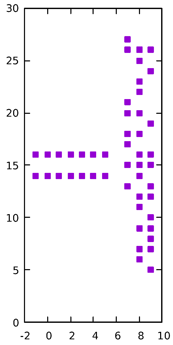
Observation 2 leads to the recognition of cases where data with high-dimensional skew cannot be clustered effectively with MD. However, some cases can still be clustered accurately if identified clusters are iteratively re-clustered in a way in which the dimensional skew is lessened. For example, Figure 2 depicts a situation where the variance of the overall data is much greater in the y direction than the x direction. Again, because depth values are scaled based on the variance of the data, a unit of Euclidean distance in the x direction yields a depth value of $0.905$ and unit of Euclidean distance in the y direction yields a depth value of $0.972$, thus, using a DBSCAN algorithm with MD cannot distinguish the two horizontal clusters without breaking apart the large vertically oriented cluster. In this case, such an algorithm can identify two clusters, the larger, vertically oriented cluster, and the other containing both horizontal point configurations on the left. Because the two horizontally oriented clusters have drastically different shape that the overall data set (their variance is much greater in the x direction as opposed to the overall data set, which has high dimensional skew in the y direction), it is possible to re-cluster those points taking into account the local shape of the cluster, a process we refer to as the Re-Cluster MD Algorithm.

The Re-Cluster MD Algorithm will first perform clustering on the overall data set, then examine each cluster and decide if it should be re-clustered based on local information. To re-cluster a cluster, we recompute the covariance matrix using only the points in the cluster, and then run the original clustering algorithm on those points using their covariance matrix for depth computations. This leads to two problems:

• Problem 1: The $\theta$ value used for the original clustering will not be relevant on the new cluster since the points will typically cover a smaller area than the original point set, and
• Problem 2: We must know when to re-cluster, and when not to.

Problem 1: Because depth values under MD are scaled by the data, if we compute depth values based on a subset of the original data, the depth values will be scaled to that subset. For example, in Figure 2, an original clustering can identify 2 clusters, the larger vertical cluster, whose points we denote $c_1$, and the two horizontal lines in a second cluster, whose points we denote $c_2$. Re-clustering $c_2$ involves computing the covariance matrix over $c_2$, and then computing depth values on those points. Depth values will then be computed by scaling Euclidean distance by this new covariance matrix; the range and density of points in $c_2$ with respect to their covariance matrix is different than the range and density of the original point set with respect to the original covariance matrix, thus a unit of depth in $c_2$ may cover a much different Euclidean distance than a unit of depth in the original data set, even if the variances of the subcluster are proportional to the variances of the original data set. Therefore, the $\theta$ value from the original clustering will not necessarily provide a good clustering when re-clustering $c_2$.

To address the issue of local depth values differing from global depth values when re-clustering, we suggest two remedies. The first is to simply choose a new value of $\theta$ for each re-clustering instance. This may prove useful in exploratory analysis, or if the densities of clusters vary greatly, but requires more fine tuning by the user. A second approach is to alter the depth computation such that the global value for $\theta$ maintains relevance when re-clustering. We use the second approach to provide a general algorithm with fewer parameters to tune. Our goal is to scale the covariance matrix of the smaller cluster based on the full point set to achieve meaningful clustering with the same depth value.

A covariance matrix for a data set can be thought of as a linear transformation from non-correlated data to the data set (or vice versa). Furthermore, a covariance matrix K for a data set is equivalent to a combination of its eigenvalues and eigenvectors; let L be a matrix with the eigenvalues of K in the diagonal, and V be the matrix with the corresponding eigenvalues in its columns:

$$K=VL{V}^{-1}$$

(9)

Intuitively, in 2-dimensional data, the eigenvectors scaled by the eignenvalues of the covariance matrix define a representative ellipse bounding (almost) the entire data set. The same concept extends to higher dimensions. The $\theta$ value used to cluster the data set is relative to depth values computed by scaling Euclidean distance along those eigenvectors with respect to those eigenvalues. When re-clustering a subset of the original data, the eigenvectors of the covariance matrix of the subset may, naturally, be different than those of the entire data set, and the eigenvalues of those eigenvectors will typically represent a smaller ellipse (in terms of area/volume), which means the depth values of two points may change drastically based on the new covariance matrix.

To remedy the change in relative depth values between points in a data set vs. points in a subset of that data when re-clustering, we take advantage of Equation (9) to scale the eigenvalues of the covariance matrix of the subset of data while maintaining the proportion of variance explained by each eigenvector. In 2-dimensional data, this (intuitively) scales the representative ellipse defined by the eigenvectors and eigenvalues of the subset of data to an ellipse with the same area of the representative ellipse defined by the original data set (or volume in higher dimensions). More generally, we propose to scale each of the eigenvalues of the covariance matrix of the subset of data by a value s such that the product of such eigenvalues is equivalent to the product of the eigenvalues of the covariance matrix of the original data set. Let D be a data set of dimension d and $D^{\prime }\subseteq D$, K and $K^{\prime }$ be the respective covariance matrices, and $e_1\dots e_d$ and $e_1^{\prime }\dots e_d^{\prime }$ be the eigenvalues of the their respective covariance matrices. We use the following formula to compute s with the goal of using the same $\theta$ on the subset of data:

$$\begin{array}{c}{s}^d\prod _{i=1}^d{e}_i^{\prime }=\prod _{i=1}^d{e}_i\hfill \\ \hfill \\ s=\sqrt[d]{{\displaystyle \frac{{\prod }_{i=1}^d{e}_i}{{\prod }_{i=1}^d{e}_i^{\prime }}}}\hfill \end{array}$$

(10)

To make the $\theta$ value used for the original clustering relevant on the smaller subset of data, we scale the eigenvalues in Equation (9) by s in Equation (10). Using this technique allows us to use the same $\theta$ value when re-examining clusters after an initial clustering.

Problem 2: In the case of MD-based clustering techniques, one does not need to re-cluster a cluster that has similar shape to the overall data set, since the Euclidean distance covered by depth values in all directions will be similar to that in the overall data set (especially once the covariance matrix for the local cluster is scaled such that the same $\theta$ value may be used). We use the term shape of the data to mean the representative ellipsoid of the data defined by the eigenvectors of its covariance matrix; for the purposes of this section, we are not concerned with scale, so the shape of two data sets may be considered identical even if their representative ellipsoids have different area/volume.

Re-clustering a subset of points can lead to poor results if a cluster has similar shape to the original data set. For example, using the data set shown in Figure 2, an initial clustering step using MD will discover 2 clusters, the vertically oriented points to the right form one cluster, and the points forming the two horizontal structures on the left of the figure. The two horizontal structures should each be identified as their own cluster (forming 3 clusters total), but because the point set is distributed in a fashion in which there is significantly higher amount of variance along the first principle component (vertical) than the second (horizontal), the two horizontal structures cannot be differentiated using MD on the entire data set. If we re-cluster the points forming the horizontal structures using MD, with the covariance matrix scaled as discussed above, we do identify both clusters using the same $\theta$ value as the original clustering. However, a problem arises in that the variances of the principle components of the vertical cluster are now even more extreme, relative to each other; the result is that a unit of depth in the horizontal direction covers so little Euclidean distance that the vertical cluster re-clusters to three clusters (respectively, the points with x an coordinate of 7, the points with an x coordinate of 8, and the points with an x coordinate of 9). Therefore, we require a mechanism to determine when a cluster should be re-clustered, and when it should not be.

We propose a mechanism to determine when a cluster should be re-clustered based on the shape of the data in a cluster as defined by its principle components relative to the shape of the overall data as defined by its principle components. Intuitively, the vertical cluster in Figure 2 should not go through a re-clustering step because it’s shape is similar to the overall shape of the data (as defined by the covariance matrices); thus, it is unlikely that the overall shape of the data is obscuring substructures in that cluster. The cluster containing the horizontal structures in Figure 2, on the other hand, has a much different shape (specifically the orientation of the principal components) than the overall data. There are various methods to compare shape of data sets in the literature (see [17,18] for a review). In order to compare the shape of data sets, we use the statistics defined in [18] that are meant to compare the shape of multivariate data sets via their covariance matrices. We choose this method because it is computationally simple, easy to interpret, produces a value as opposed to a strict classification, and does not depend on distributional assumptions. We summarize the statistics in the remainder of this section.

Let $D_1$ and $D_2$ be two multivariate point sets and $X_1$ and $X_2$ be matrices, respectively, containing the eigenvectors of the covariance matrices of $D_1$ and $D_2$. $X_1$ and $X_2$ are organized such that the eigenvectors are in their columns. Let $cov\left(\right)$ be a function that computes the covariance matrix of a data set.

$$\begin{array}{ccc}{C}_{11}=cov\left(D_1{X}_1\right)\hfill & \hfill & C_{22}=cov\left(D_2{X}_2\right)\hfill \end{array}$$

(11)

The variances in $C_{11}$ are the eigenvalues of the of the principle components of the original data (likewise for $C_{22}$). In other words, those values indicate the amount of variance explained by the eigenvectors indicating the principle components of the original data. Similarly:

$$\begin{array}{ccc}{C}_{12}=cov\left(D_1{X}_2\right)\hfill & \hfill & C_{21}=cov\left(D_2{X}_1\right)\hfill \end{array}$$

(12)

The variances in $C_{12}$ indicate the amount of variance from data set $D_1$ explained by the eigenvectors representing the principle components of $D_2$ (likewise for $C_{21}$). For each dimension of the data, let:

$$\begin{array}{ccc}{v}_{i11}=C_{11}[i,i]\hfill & \hfill & v_{i22}=C_{22}[i,i]\hfill \\ v_{i12}=C_{12}[i,i]\hfill & \hfill & v_{i21}=C_{21}[i,i]\hfill \end{array}$$

(13)

where $v_{i11}$ is the amount of total variance in $D_1$ explained by the $ith$ eigenvector in $X_1$, $v_{i12}$ is the amount of total variance in $D_1$ explained by the $ith$ eigenvector in $X_2$, etc. Using these values, one may compute the following statistic for n-dimensional data:

$$S=2\sum _{i=1}^n{(v_{i11}-v_{i21})}^2+{(v_{i12}-v_{i11})}^2$$

(14)

For our purposes, we do not require the sum be multiplied by 2, but we keep it such that the statistic fits within the framework defined in [18]. Intuitively S in Equation (14) is a measure of the difference of the ability of the eigenvectors of the covariance matrix from one data set to explain the variation in the other data set, and vice versa. As constructed, Equation (14) has two properties that are not desirable for our purposes. First, the statistic is sensitive to the magnitude of the eigenvectors used. In other words, a data set with small range and a data set with large range will compute as being different. Second, the value produced is not bounded in a way to make comparisons easy. Both of these properties are addressed if instead of using the raw variances for the various v values in Equation (13), we express each value as a proportion of total variance explained; thus, covariance matrix differences are computed on orientation of the eigenvectors, and proportion of the eigenvalues (meaning two covariance matrices covering the same data, but at difference scales, are considered equivalent).

Finally, the maximum value of S in Equation (14) when expressing variance explained as proportion of total variance is 8, and occurs in the case when single eigenvectors explain all the variance in each sample, and those eigenvectors are orthogonal. Likewise, a value of 0 occurs when $D_1=D_2$. It is useful to have similarity values range from $0-1$, and since we are in the context of depth calculations where a depth of 1 indicates identity, we will express the statistic from Equation (14) as the following:

$$S=1-\left({\displaystyle \frac{2{\sum }_{i=1}^n{(v_{i11}-v_{i21})}^2+{(v_{i12}-v_{i11})}^2}{8}}\right)$$

(15)

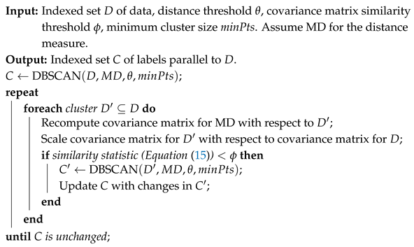
We incorporate covariance matrix similarity comparisons with DBSCAN using MD in order to achieve an algorithm able to re-cluster point clusters with covariance matrices that are different in shape than the matrix of the overall data and that is robust in its parameterization. We introduce a new user-defined variable, $\varphi$ that represents a covariance matrix similarity threshold. A cluster will be re-clustered based on its scaled MD value if its covariance matrix similarity value as compared to the data set from which the cluster was identified is below $\varphi$. The algorithm is presented in Algorithm 2.

Algorithm 2 essentially performs repeated DBSCAN algorithms on increasingly smaller subsets of the data until no new clusters are found. The time complexity of optimal DBSCAN is $O(nlgn)$. In the worst possible case, the DBSCAN algorithm would result in 2 clusters, one consisting of the minimal number of points in a cluster, then the other containing the remaining points that must be re-clustered. This pattern could repeat, essentially leading to $\left(O{(nlgn)}^2\right)$. In practice, such a degenerate case would require high dimensionality to be possible, since the shape of each successively smaller cluster would need to change enough to reveal clusters with respect to different dimensions, and is unlikely. In the experiments in this paper, only a single re-clustering step is necessary.

Algorithm 2: Algorithm to re-cluster initial clusters from an MD-based DBSCAN

5. Experiments

In this section, we confirm the mathematical properties discussed previously via experiments. We conduct experiments to investigate the affect of data shape on MD-based algorithms, the robustness of clustering algorithms to noise, the behavior of clustering algorithms with respect to affine transformations of data (Synthetic data created with MLBench), and finally we compare the algorithms on multivariate data sets from the UCI Machine Learning Repository [19]. The algorithms used in the experiments are the traditional DBSCAN, DBCA, CRAD; and the proposed algorithms are PD (DBSCAN using PD), DBCA w/minPts (DBSCAN with MD), and Re-cluster MD. We attempt to achieve the parameterization providing best results for each algorithm by narrowing in on parameters by hand, using multiple combinations. The effect of the $\varphi$ parameter for the Re-cluster MD algorithm is to limit reclustering attempts, and thus is not very sensitive. If $\varphi$ is too high, this means that more clusters will go through re-clustering process with little likelihood of new clusters being found; in other words, a poor choice can lead to more computation time. We choose a conservative value for our experiments. CRAD provides an optimal range for the number of bins parameter, so we chose 20 evenly-spaced values in the range since performance was highly variable among parameters; this allows us to explore values from the entire suggested range. Adjusted Rand Index (ARI) and Variation of Information (VI) scores are reported. We used our own implementations of all algorithms except for the CRAD algorithm. For CRAD, we used the code made available by the authors of [3] in a git repository (https://github.com/DataMining-ClusteringAnalysis/CRAD-Clustering, accessed on 1 July 2025).

5.1. High Dimensional Skew

Figure 3 depicts a data set with high-dimensional skew. This example is constructed to highlight the properties of MD-based algorithms in which a unit of depth results in vastly different Euclidean distance depending on the direction.

Table 1. Results for data shown in Figure 3.

	ARI	VI
Re-cluster MD	1	0
PD	0.88	0.268
DBSCAN	0.883	0.252
DBCA	0.868	0.285
DBCA (w/ minPts)	0.868	0.285
CRAD	0.783	0.473

indicates the results of the clustering algorithms over this data set. Most algorithms perform well, but have trouble with the horizontally oriented clusters in the lower right, with the exception of perfect clustering by the Re-cluster MD algorithm. PD and traditional DBSCAN preform well, since they are not affected by high-dimensional skew in the same way as MD-based algorithms. The MD based algorithms without re-clustering, predictably, perform the worst.

5.2. Noise

Figure 4 depicts the synthetic data used for noise and affine transformation experiments. For noise, we added 5–50% noise in increments of 5 to the data set (i.e., the original data set has 6300 points and the data set with $50\%$ noise has 12,600 total points where 6300 of them are noise). For example, the $25\%$ noise data set is shown in Figure 5.

Results are depicted in Figure 6. Most of the algorithms performed very similarly except for two: CRAD and DBCA. Of the algorithms that perform similarly, we observe a gradual decrease in correct clustering as noise is increased, showing a graceful degradation as noise increases. To achieve these scores, the minPts parameter began at 3 and was increased to 4 as noise increased. DBCA’s performance diverges from the others because, as presented in [2], the DBCA algorithm does not have a minPts parameter. By incorporating MD into a traditional DBSCAN algorithm (DBCA w/minPts), we achieve better results.

Although CRAD uses MD, it identifies clusters based on changes in density in what is effectively a one-dimensional data projection. Predictably, the introduction of noise has great effect on this style of clustering. At $10\%$ noise, the performance of CRAD drastically diminishes.

5.3. Affine Transformations

To test the performance of the algorithms under affine transformations, we apply affine transformations to the original data set in Figure 4. Eleven data sets are used in the experiments, numbered as follows: (0) original data set; (1) translate: x-axis by 10; (2) reflect: x-axis; (3) rotate: $-{45}^{\circ }$; (4) scale: x- and y-axis by a factor of 7; (5) scale: y-axis by a factor of $0.5$; (6) shear: y-axis by a factor of $0.5$; (7) rotate: $-{30}^{\circ }$/scale: x-axis by a factor of $0.6$; (8) shear: y-axis by a factor of $0.5$/rotate: ${45}^{\circ }$; (9) reflect: x-axis/shear: y-axis by a factor of $0.8$; and (10) translate: x-axis by 10/reflect: x-axis/shear: x-axis by a factor of $0.8$/scale: x-axis by a factor of $2.5$/rotate: ${45}^{\circ }$. The numbers in the x-axis of Figure 7 correspond to the data set numbers described here. Figures of the transformed data sets appear in Appendix A.

We say that a clustering algorithm is invariant to affine transformations if it clusters data identically both before and after affine transformations while using the same parameters. Clearly, DBSCAN is does not fit this definition since scaling the data requires manipulating the $\theta$ value to reflect the new distances between data points. Figure 7 shows the results. Indeed, MD-based clustering techniques cluster data identically under affine transformations using the same parameters. This follows from the fact that distance values are scaled to depth values based on the variance of the data under MD. DBSCAN returns identical clustering under translations, rotations, and reflections, but fails when data is scaled. PD returns identical clustering under translation, rotation, reflection, and scale, as long as all axes are scaled identically. Shear or scale that is not identical on all axes may cause the first principal component to change direction or magnitude from the original data, requiring parameter adjustment.

5.4. Multivariate Data

Results of the algorithms run on real-world, multivariate data sets [19] are shown in

Table 2. Results of the multivariate data sets.

	Adjusted Rand Index
	Re-cluster MD	PD	DBSCAN	DBCA	DBCA (w/ minPts)	CRAD
Iris	0.53	0.568	0.568	0.529	0.53	0.537
Banknote	0.769	0.534	0.558	0.769	0.769	0.443
Occupancy	0.607	0.93	0.93	0.607	0.607	0.099
Seeds	0.214	0.385	0.385	0.196	0.214	0.138
Blood Transfusion	0.023	0.031	0.037	0.024	0.023	0.051
	Variation of Information
	Re-cluster MD	PD	DBSCAN	DBCA	DBCA (w/ minPts)	CRAD
Iris	1.12	0.667	0.667	1.15	1.12	0.888
Banknote	0.902	1.352	1.097	0.923	0.902	1.659
Occupancy	1.031	0.232	0.232	1.032	1.031	2.988
Seeds	2.252	2.619	2.619	2.519	2.252	3.647
Blood Transfusion	0.954	0.869	0.863	0.956	0.954	1.194

. We choose these data sets because they are used for reporting on CRAD and DBCA in the literature [3] and the ground truth is known. These data sets have either 2 or 3 clusters, and dimensionality of 4–7. It turns out that none of these data sets have dimensional skew high enough to require re-clustering, therefore, the Re-cluster MD results are identical to DBCA with minPts. Furthermore, some data sets achieved highest performance with the lowest minPts setting, so that DBCA returns identical results to DBCA with minPts.

In general PD and DBSCAN are able to achieve identical clustering with the right parameterizations. As shown, we achieve identical results, or very close results with our method of exploring parameters. Thus, when DBSCAN performs the best, it ties with PD. The advantage of PD is that it is stable under some affine transformations of data. These algorithms perform the best on 3 of the 5 data sets, significantly outperforming the others in the Occupancy data set.

The MD-based DBSCAN algorithms perform best on the Banknote data set, most likely due to the data favoring the elliptical scaling of variance provided by MD. A possible reason why the MD-based DBSCAN did not perform better on other data sets is that there is skew present in the overall shape of the data, but clusters within the data generally do not have a skewed shape. This is suggested in the results since DBSCAN and PD, which do not consider skew, did quite well in those data sets.

All algorithms performed poorly on the blood transfusion data set; thus it is tough to draw conclusions.

5.5. Roadway Data

A motivating example of our work is data along roadways where clusters may be greatly skewed in one direction, leading to points being clustered together when they lie along different roadways. Figure 8 depicts the locations of bridges around the city of St. Louis (Data from U.S. Federal Highway Administration National Bridge Inventory: https://catalog.data.gov/dataset/national-bridge-inventory-abd5a, accessed on 1 July 2025). Clusters in the data will occur along roadways or at the intersection of roadways. One problematic area is near the left side of the image where there is an East–West oriented cluster of bridges along the highway, and another small cluster above it along some train tracks that run very near the highway. In order for traditional DBSCAN to be able to differentiate those clusters, the distance value has to be set so small that many points are considered noise and clusters are lost (Figure 9). DBSCAN using projection depth yields the same result as Euclidean distance in this case since distance is weighted identically in all directions. Using MD and re-clustering, we are able to differentiate those clusters while maintaining meaningful clustering. Furthermore, the clusters using MD and re-clustering results in clusters that more closely align with the underlying roadway structure (i.e., elongated clusters) (Figure 10).

As a final example, Figure 11 and Figure 12 depict clustering results using HDBSCAN [20]. HDBSCAN is able to handle clusters with varying densities, unlike traditional DBSCAN, but does not take into account dimensional skew. We were unable to find a combination of parameters that differentiated the bridges on the train tracks and the highways mentioned above. Using a minimum cluster size of 4 (Figure 11), the algorithm struggles with the varying densities of bridge locations, breaking up clusters that are near and along the same roadway, but having different densities (see points on the left side of the image, creating different clusters along the same highway, or towards the center of the image). Increasing the minimum cluster size parameter to 5 (Figure 12) creates clusters that include points from multiple roadways and train tracks.

6. Conclusions

We examined previous work using data depth measures in density-based clustering and identified properties of those measures that may be problematic in certain situations. We then introduced three new approaches to data depth clustering: using projection depth, using an adaptive Re-clustering technique for MD-based algorithms that overcomes issues arising from high-dimensional skew in data, and parameterizing DBCA with a minPts parameter to match DBSCAN style algorithms more closely and allow more resilience to noise. Finally, we evaluated the new algorithms and compared them to existing algorithms using data sets to test adaptability to high-dimensional skew, noise, affine transformations, and performance on real-world, multivariate data. PD performs identically to DBSCAN, but is robust under the affine transformations of translation, rotation, and identical scaling along all dimensions; therefore, it is a good choice for applications such as data collected from drones that may fly at differing altitudes over the same area. The MD Re-clustering technique effectively deals with with dimensional skew in clusters, but can struggle in cases where clusters are not skewed but the overall data shape has skew, leading to missing clusters in the first clustering round. However, some situations arise where the skew of the overall data shape causes clusters to have skew as well (e.g., the roadway data set based on latitude and longitude coordinates); the MD Re-clustering performs well in such cases. Thus, we have provided an expanded set of tools for practitioners to use that are grounded in well established techniques, and can be effectively leveraged with knowledge of the application domain. Future work includes the consideration of additional depth measures, studying mechanisms to alter PD to more effectively handle skew transformations, and studying additional mechanisms to address dimensional skew in MD algorithms.

References

1. Ester, M.; Kriegel, H.P.; Sander, J.; Xu, X. A density-based algorithm for discovering clusters in large spatial databases with noise. In Proceedings of the Second International Conference on Knowledge Discovery and Data Mining, Portland, OR, USA, 2–4 August 1996; Volume 96, pp. 226–231. [Google Scholar]
2. Jeong, M.H.; Cai, Y.; Sullivan, C.J.; Wang, S. Data depth based clustering analysis. In Proceedings of the 24th ACM SIGSPATIAL International Conference on Advances in Geographic Information Systems, San Francisco, CA, USA, 31 October–3 November 2016; pp. 1–10. [Google Scholar]
3. Huang, X.; Gel, Y.R. Crad: Clustering with robust autocuts and depth. In Proceedings of the 2017 IEEE International Conference on Data Mining (ICDM), New Orleans, LA, USA, 18–21 November 2017; pp. 925–930. [Google Scholar]
4. Mahalanobis, P.C. On the Generalized Distance in Statistics; National Institute of Science of India: Jatani, India, 1936. [Google Scholar]
5. Donoho, D.L.; Gasko, M. Breakdown properties of location estimates based on halfspace depth and projected outlyingness. Ann. Stat. 1992, 20, 1803–1827. [Google Scholar] [CrossRef]
6. Tukey, J.W. Exploratory Data Analysis; Addison-Wesley: Reading, MA, USA, 1977; Volume 2. [Google Scholar]
7. Liu, R. Data depth and multivariate rank tests. In L1-Statistical Analysis and Related Methods; North-Holland: Amsterdam, The Netherlands, 1992; pp. 279–294. [Google Scholar]
8. Hartigan, J.A.; Wong, M.A. A K-means clustering algorithm. J. R. Stat. Soc. Ser. (Appl. Stat.) 1979, 28, 100–108. [Google Scholar]
9. MacQueen, J. Some methods for classification and analysis of multivariate observations. In Proceedings of the Fifth Berkeley Symposium on Mathematical Statistics and Probability, Oakland, CA, USA, 27 December 1965–7 January 1966; Volume 1, pp. 281–297. [Google Scholar]
10. Cerioli, A. K-means cluster analysis and mahalanobis metrics: A problematic match or an overlooked opportunity. Stat. Appl. 2005, 17, 61–73. [Google Scholar]
11. Melnykov, I.; Melnykov, V. On K-means algorithm with the use of Mahalanobis distances. Stat. Probab. Lett. 2014, 84, 88–95. [Google Scholar] [CrossRef]
12. Zuo, Y.; Serfling, R. General notions of statistical depth function. Ann. Stat. 2000, 28, 461–482. [Google Scholar] [CrossRef]
13. Mosler, K. Depth statistics. In Robustness and Complex Data Structures; Springer: Berlin/Heidelberg, Germany, 2013; pp. 17–34. [Google Scholar]
14. Van Aelst, S.; Rousseeuw, P. Minimum volume ellipsoid. Wiley Interdiscip. Rev. Comput. Stat. 2009, 1, 71–82. [Google Scholar] [CrossRef]
15. Hubert, M.; Debruyne, M. Minimum covariance determinant. Wiley Interdiscip. Rev. Comput. Stat. 2010, 2, 36–43. [Google Scholar] [CrossRef]
16. Rousseeuw, P.J.; Driessen, K.V. A fast algorithm for the minimum covariance determinant estimator. Technometrics 1999, 41, 212–223. [Google Scholar] [CrossRef]
17. Steppan, S.J.; Phillips, P.C.; Houle, D. Comparative quantitative genetics: Evolution of the G matrix. Trends Ecol. Evol. 2002, 17, 320–327. [Google Scholar] [CrossRef]
18. Garcia, C. A simple procedure for the comparison of covariance matrices. Bmc Evol. Biol. 2012, 12, 222. [Google Scholar] [CrossRef] [PubMed]
19. Dua, D.; Graff, C. UCI Machine Learning Repository; UC Ivine: Irvine, CA, USA, 2017. [Google Scholar]
20. Campello, R.J.; Moulavi, D.; Sander, J. Density-based clustering based on hierarchical density estimates. In Proceedings of the Pacific-Asia Conference on Knowledge Discovery and Data Mining, Gold Coast, Australia, 14–17 April 2013; pp. 160–172. [Google Scholar]
Figure 1. A data set with two clusters (one purple and one red). Using MD with a DBSCAN algorithm, the two clusters cannot be distinguished.
Ijgi 14 00298 g001
Figure 2. A data set with three clusters such that two clusters are oriented perpendicular to the general orientation of the data.
Ijgi 14 00298 g002
Figure 3. The re-clustering data set. A total of 1600 points and 13 clusters.
Ijgi 14 00298 g003
Figure 4. The original synthetic data set. A total of 6300 points and 13 clusters.
Ijgi 14 00298 g004
Figure 5. An example of one of the noise data sets. This data set has 25 % of the total points being noise.
Ijgi 14 00298 g005
Figure 6. Results for varying percentages of noise added to the original synthetic data set (Figure 4).
Ijgi 14 00298 g006
Figure 7. Results for several different affine transformations performed on the original synthetic data set (Figure 4).
Ijgi 14 00298 g007
Figure 8. Locations of Bridges around the city of St. Louis.
Ijgi 14 00298 g008
Figure 9. Clustering using DBSCAN with Euclidean distance. To differentiate two clusters (one along the highway and the other along the railroad tracks in the left of the image), the distance value must be set such that many other clusters are lost and many points are considered noise. Clustering with Projection Distance yields identical results.
Ijgi 14 00298 g009
Figure 10. Clustering using DBSCAN with MD. As opposed to Euclidean Distance, MD clusters based on the elongated shape of roadways and can differentiate clusters that Euclidean distance cannot while maintaining good clustering of the remaining data.
Ijgi 14 00298 g010
Figure 11. Clustering using HDBSCAN with minimum cluster size parameter set to 4.
Ijgi 14 00298 g011
Figure 12. Clustering using HDBSCAN with minimum cluster size parameter set to 5.
Ijgi 14 00298 g012