Article

A Novel Method for Estimating Building Height from Baidu Panoramic Street View Images

1
Research Center of Geospatial Big Data Application, Chinese Academy of Surveying and Mapping, Beijing 100036, China
2
Department of Geography, Ghent University, 9000 Ghent, Belgium
*
Author to whom correspondence should be addressed.
ISPRS Int. J. Geo-Inf. 2025, 14(8), 297; https://doi.org/10.3390/ijgi14080297
Submission received: 20 May 2025 / Revised: 22 July 2025 / Accepted: 28 July 2025 / Published: 30 July 2025

Abstract

Building height information plays an important role in many urban-related applications, such as urban planning, disaster management, and environmental studies. With the rapid development of real scene maps, street view images are becoming a new data source for building height estimation, considering their easy collection and low cost. However, existing studies on building height estimation primarily utilize remote sensing images, with little exploration of height estimation from street-view images. In this study, we proposed a deep learning-based method for estimating the height of a single building in Baidu panoramic street view imagery. Firstly, the Segment Anything Model was used to extract the region of interest image and location features of individual buildings from the panorama. Subsequently, a cross-view matching algorithm was proposed by combining Baidu panorama and building footprint data with height information to generate building height samples. Finally, a Two-Branch feature fusion model (TBFF) was constructed to combine building location features and visual features, enabling accurate height estimation for individual buildings. The experimental results showed that the TBFF model had the best performance, with an RMSE of 5.69 m, MAE of 3.97 m, and MAPE of 0.11. Compared with two state-of-the-art methods, the TBFF model exhibited robustness and higher accuracy. The Random Forest model had an RMSE of 11.83 m, MAE of 4.76 m, and MAPE of 0.32, and the Pano2Geo model had an RMSE of 10.51 m, MAE of 6.52 m, and MAPE of 0.22. The ablation analysis demonstrated that fusing building location and visual features can improve the accuracy of height estimation by 14.98% to 69.99%. Moreover, the accuracy of the proposed method meets the LOD1 level 3D modeling requirements defined by the OGC (height error ≤ 5 m), which can provide data support for urban research.

1. Introduction

Building height data plays a crucial role in 3D smart city modeling [1], urban planning [2], urban safety [3], population estimation [4], and many other innovative urban applications. Traditional building height estimation primarily uses remote sensing data, including optical images [5,6], synthetic aperture radar (SAR) images [7,8], and aerial LiDAR data [9]. The use of remote sensing data has the advantage of allowing the rapid estimation of building heights within a large area, but it also has some limitations. For example, optical image-based methods are susceptible to light and weather conditions at the time of image capture [10]. SAR-image-based methods are susceptible to different microwave scattering mixes, which leads to high uncertainty in the estimation results [11]. LiDAR-based methods can provide high-precision building height information; however, the results are discrete and require further processing [9].
Compared to remote sensing and oblique imagery (UAV-based aerial photogrammetry), street-view imagery has significant advantages for building height estimation. First, its unique ground-level- perspective captures details such as building facades, windows, and roof contour lines, providing a more refined data foundation for height feature recognition. Kim & Han [12] leveraged facade features from street-view images to achieve height estimation. In contrast, oblique imagery can capture the facade geometry through multi-angle shots, but its resolution is constrained by flight altitude, making its facade capturing capability inferior to that of street-view imagery. Second, street view imagery offers cost effectiveness: compared to high-resolution remote sensing, LiDAR, and UAV-based aerial photogrammetry, its acquisition cost is significantly lower [13]. Street-view data for many cities can be accessed for free through open platforms such as Baidu Street View and Tencent Street View. Long & Liu [14] collected over one million street view images to analyze urban street greening conditions. Feng et al. [15] crawled over ten thousand street view images via open platform APIs to investigate the urban heat island effect. This avoids the expensive equipment investment of drones, complex flight permit applications, mission planning, and personnel qualification requirements. Third, street view coverage is extensive and readily accessible, now reaching the county level in China, making it well-suited for large-scale applications, whereas UAV-based aerial photogrammetry is often constrained by regulations and site operation limitations. Finally, street view data exhibit greater stability: unlike remote sensing imagery, which is susceptible to interference from clouds and shadows, street view images are typically captured under favorable weather conditions, making them less affected by environmental factors and more consistently available.
With the rapid development of image segmentation and Street View maps, street view imagery has begun to be used in studies on building height estimation. Based on the field of view (FOV) of the street-view imagery, we categorized the building height estimation methods for perspective street-view imagery (FOV < 180°) and panoramic street-view imagery (FOV = 360°), as detailed in Table 1.
The methods for perspective street-view imagery can be divided into three categories. The first category is single-view geometry, which uses a camera projection model to estimate building heights. Zhao et al. [16] combined deep learning with the camera projection model to propose a CBHE framework for collaborative detection of building corner points and rooflines, which supports height estimation of individual buildings while improving estimation accuracy. However, when buildings are located in densely built-up areas, the estimation errors increase. Al-Habashna [17] simplified the roofline extraction process of the CBHE framework proposed in [16] to make it more practical, but this approach is prone to errors due to vegetation occlusion. Díaz & Arguello [18] first proposed a method for estimating the average height of buildings using Google Street View imagery and validated it with a prototype system. However, this method does not support the estimation of the height of a single building. The second category estimates building heights by exploiting the pixel-height ratio between objects of known physical height and buildings in the image. Ureña-Pliego [19] used vehicles as reference objects to calculate building heights based on proportional relationships. The accuracy of this method is sufficient for earthquake emergency response; however, it requires the reference object to be adjacent to the building. Furthermore, the estimated height represents the average height of all buildings in the street-view image rather than the height of a single building. The third category leverages multimodal feature fusion using various building characteristics (geometric and semantic) to train machine learning models for building height estimation. Li et al. [20] implemented large-scale building height estimation by utilizing building features from OpenStreetMap and Mapillary street view images, and generated LOD1 3D building models. However, this method relies on 129 features and is difficult to apply in areas where OpenStreetMap data are lacking.
There is only one category of methods for panoramic street view imagery, which is single-view geometry. Fan et al. [21] proposed Pano2Geo, a pixel-level 3D geographic coordinate projection model based on panoramic imagery, and introduced the NENO rules and the art gallery theorem to optimize panorama acquisition strategies, reducing street view data redundancy and improving height estimation accuracy. However, this method does not account for the impact of terrain undulation on height estimation, and large slope variations can result in significant errors in the estimation. Ning et al. [22] employed a YOLO network to measure the height of buildings’ ground-floor doors, thereby estimating the lowest-floor height, and applied this approach to flood vulnerability assessment. Ho et al. [23] introduced depth maps from Google Street View into the study of lowest-floor height estimation, enhancing estimation accuracy. Ho et al. [24] introduced the Segment Anything Model and vision-language models into the study of lowest-floor height estimation, further improving estimation accuracy. However, studies [22,23,24] focused on the lowest-floor height estimation rather than the overall building height, and the only method capable of estimating the full building height is the Pano2Geo model.
To extend the building height estimation methods in panoramic images, we developed a novel building height estimation framework based on Baidu panoramic images. Inspired by Li et al. [20], we proposed a two-branch feature fusion network that integrates building location and visual features extracted from panoramic images to estimate the height of individual buildings. Unlike Li et al. [20] who relied solely on morphological features of buildings for height estimation, we introduced a visual feature branch that encodes texture and deep semantic information from street view images into feature vectors, which are then fused with the building location branch, thus expecting to improve the accuracy of building height estimation.

2. Materials and Methods

2.1. Study Area

This study used the Fengtai District of Beijing as the study area. Fengtai is located in southwest Beijing and has many types and numbers of buildings with large height variations. We collected building footprint data with height attributes for Beijing from Baidu Maps [25]. By computing the Kullback-Leibler Divergencen [26] (hereinafter referred to as KL divergence), we analyzed the consistency of building height distributions between four urban districts (Haidian, Chaoyang, Shijingshan, and Fengtai) and the entire Beijing area. KL divergence is an asymmetric indicator that measures the difference between two probability distributions. The closer the value is to zero, the smaller the difference between the two distributions. The calculation results show that Fengtai District has the smallest KL divergence value of 0.0026, which indicates that the Fengtai District can typically represent the building height distribution of Beijing.
The distribution of building heights in the study area is shown in Figure 1. Buildings exceeding 100 m account for only 1% of the total number of buildings. Therefore, they were not included in this study.

2.2. Data Collection

Street-view platforms in China are primarily represented by Baidu Maps and Tencent Maps. The Baidu street view covers more than 600 cities in China [27] and continuously updates street view images. In contrast, Tencent Maps’ street view service has not updated its street view data since 2021 [28]. Given these considerations, Baidu Maps was selected as the optimal street-view data source for this study.
As street view images are usually captured along roads, to ensure that there are street view images near buildings, we conducted a 50-m buffer zone analysis on the Fengtai road network and obtained the buildings within the buffer zone. Stratified sampling of buildings within the buffer zone by height ensured 50 building samples per stratum. A 50-m buffer analysis was conducted for each building sample, and 25 points were uniformly sampled within the buffer as street view sampling points for that sample. Finally, panoramic images and metadata were collected using the Baidu Maps Application Programming Interface (API) [25] based on the geographic coordinates of the street view sampling points. Because green trees may block buildings during warm seasons, we only collected street-view images during the cold months, i.e., January, February, November, and December of each year. In total, we collected 1650 building samples.

2.3. Methods

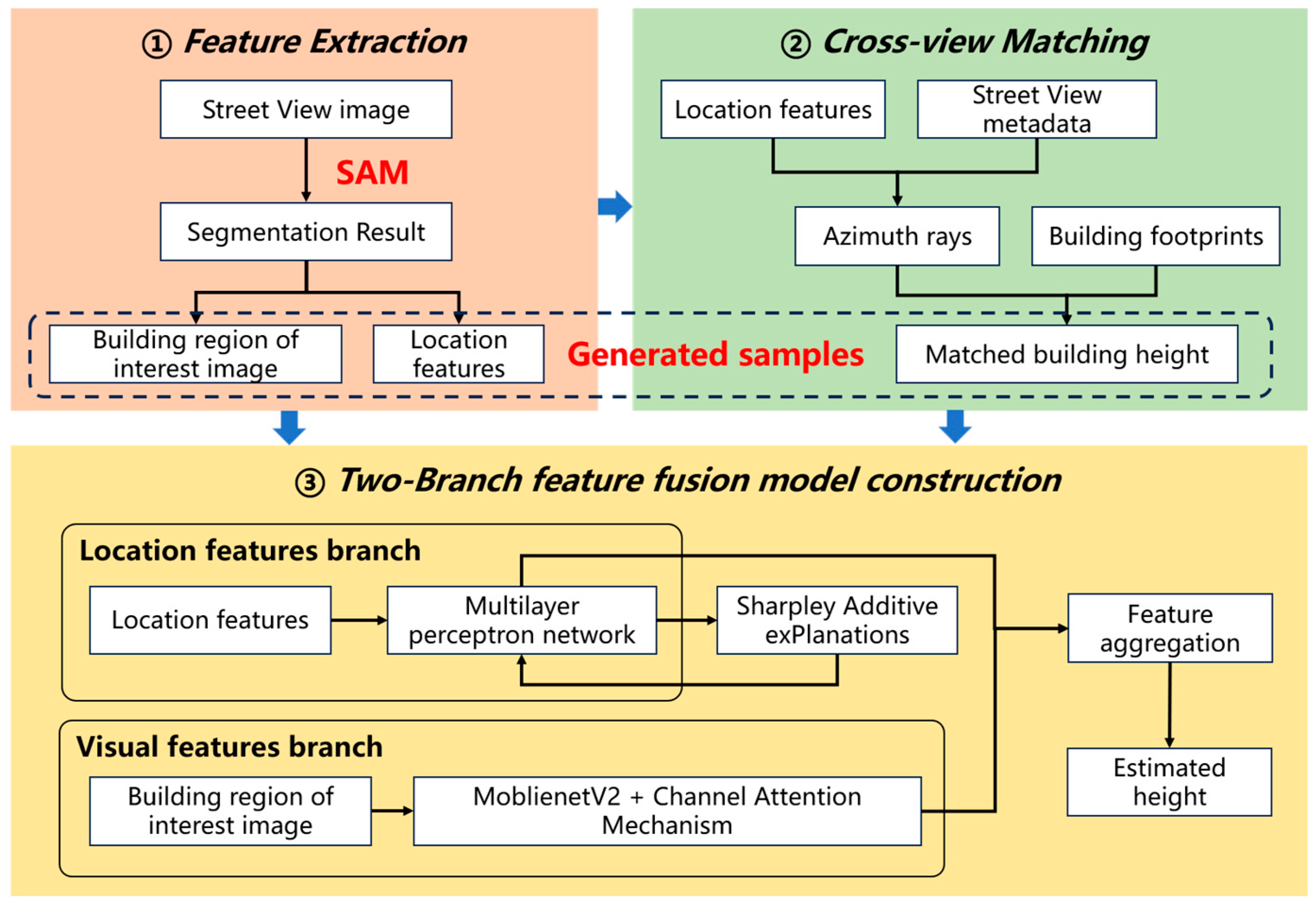
We proposed a novel method for estimating building height using Baidu panoramic street view images, which includes three parts. Firstly, the Segment Anything Model (hereinafter referred to as SAM) was used to extract the building region of interest (ROI), and location features were manually designed based on these ROIs. Subsequently, a cross-view matching strategy was explored to assign height attributes to single buildings in panoramic images using building footprint data with height information, thereby reducing the annotation time required for the height samples. Afterwards, a two-branch feature fusion (TBFF) model was constructed by integrating the building location and visual features, and its performance was compared and evaluated to achieve a satisfactory building height estimation using panoramic images. The specific flow of this method is shown in Figure 2.

2.3.1. Building Region of Interest and Location Features Extraction

We used the SAM to extract the building region of interest in panoramic images. SAM is a highly flexible model developed by Meta AI that performs image segmentation tasks that aim to “segment anything” within an image, automatically or based on user inputs, using an advanced deep learning model. The SAM has three main components: a powerful image encoder, a prompt encoder, and a mask decoder [29]. The SAM first encodes the input image and then extracts the mask based on the prompt information. Finally, the mask is decoded and the output is generated. The SAM can generalize across a wide range of segmentation tasks without requiring retraining on specific datasets [30]. Therefore, SAM was directly implemented to obtain the outlines of each object within the street-view image, and the building objects were visually labelled.
Numerous studies have proven that the location of a building within an image is closely related to its actual height [16,17]. Therefore, we designed eight location features to represent the locations of buildings in panoramic images (Figure 3). They include the width (Wb) and height (Hb) of the building’s bounding box, the horizontal distance (Xc) and vertical distance (Yc) distances from the bounding box center to the image’s upper left corner, the horizontal distance (Xtl) and vertical distance (Ytl) from bounding box’s upper left corner to the image’s upper left corner, as well as the horizontal distance (Xrb) and vertical distance (Yrb) from bounding box’s bottom right corner to the image’s bottom right corner. All location features are measured in image pixels and then normalized to [0,1] by the width or height of the image. There may be redundant features among the eight features, which will increase the risk of overfitting the model and require the use of feature selection strategies. Guyon & Elisseeff [31] demonstrated that feature selection aims to improve the model performance and feature interpretability. Marcilio & Eler [32] adopted Shapley Additive Explanations (SHAP) as a feature selection strategy and experimentally demonstrated its superiority over other common feature selection methods on medical datasets. SHAP is a framework that can explain machine learning models. SHAP assigns the importance of each feature to the prediction result based on the Shapley value in game theory. At the same time, it is not limited by the model type and is applicable to all black box models [33]. SHAP provides transparent and reliable explanation mechanisms that help researchers in disciplines such as geography [34], architecture [35], and medicine [36] to understand model decision-making processes. In summary, we employed SHAP to explain the importance of the location features and remove redundant features.

2.3.2. Cross-View Matching Between Street View Images and Building Footprints

Following the extraction of the building’s region of interest and location features, it is necessary to match them with building footprint data with known height information. The building region of interest in the panoramic image is from the facade view, while the height information from the building footprint data is from the overhead view. Thus, it is difficult to match them visually due to the different perspectives. The matching interpreters depend on knowledge of the building footprint, surrounding roads, and building orientations to find the correct building region of interest for each building footprint, which is time-consuming. Ogawa et al. [37] have proposed a method to associate street view images with spatial data by firstly calculating the horizontal angle range of buildings in the panorama, then combining the building footprint data and street view metadata to calculate the angle range of the building footprint at a specific street view sampling point, and finally comparing the above two angles to realize the matching. However, this method cannot be directly used for Baidu Street View because of the differences in the street view metadata. Inspired by this, we propose a cross-view fast matching algorithm for Baidu Street View and spatial footprint data. Figure 4 illustrates the workflow of our cross-view matching algorithm.
Initially, the horizontal azimuth range of the building within a panoramic image is calculated based on the extracted horizontal location features of the building and street view metadata, including heading information and coordinates of the street view image. The calculation formula is shown in Equation (1), θ r a n g e represents the horizontal azimuth range of the building, θ l e f t represents the horizontal azimuth of the left boundary of the building facade, and θ r i g h t represents the horizontal azimuth of the right boundary of the building facade.
θ r a n g e = θ r i g h t θ l e f t
Specifically, the heading information represents the azimuth corresponding to the forward direction of the street-view collection vehicle, ranging from 0° to 360°. The horizontal azimuth tends to be calculated along the clockwise direction from the north direction, and the azimuth angle ( θ i m g c e n t e r ) corresponding to the center of the image is always perpendicular to the forward direction of the front end of the vehicle and is located on the left side of the forward direction of the front end of the vehicle. Figure 5 illustrates the relationship between these two azimuth angles. In Figure 5, the sky blue line represents the street view capture vehicle’s forward direction, and the yellow line represents θ i m g c e n t e r . Thus, we calculated θ i m g c e n t e r using Equation (2) according to the rules of the azimuth angle calculation, where h e a d i n g represents the street view capture vehicle’s forward direction. Then, the azimuth ( θ c e n t e r ) corresponding to the center of the building facade, θ l e f t and θ r i g h t can be calculated using the horizontal location features Xc, Xtl, and Xrb (Equations (3)–(5)). Where 0.5 represents the normalized width corresponding to the center of the image.
θ i m g e c e n t e r = h e a d i n g 90 °
θ c e n t e r = θ i m g c e n t e r + ( X c 0.5 ) × 360 °
θ l e f t = θ i m g c e n t e r + ( X t l 0.5 ) × 360 °
θ r i g h t = θ i m g c e n t e r + ( 0.5 X r b ) × 360 °
Subsequently, based on the geographic coordinates of the street-view image and the calculated horizontal azimuth range of the building, the azimuth rays are generated, and the footprint of the building intersecting the ray can be found by intersecting it. There are more than 80,000 buildings in the study area, and the time complexity of the matching algorithm will be high if the azimuth rays intersect with each building. We used Rtree to construct a spatial index for each building footprint to reduce the time complexity of the cross-view matching algorithm. Rtree, a commonly used spatial indexing structure, is well suited for indexing and querying 2D and 3D data in the field of GIS, with a time complexity of O(log n) [38].
The matching steps are as follows: Firstly, we used θ c e n t e r to construct an azimuth ray to intersect the building footprints; if there is an intersection, then no other angle range is used. Otherwise, we gradually increased the ray’s angle from θ l e f t to θ r i g h t by one degree to construct multiple rays that intersected with the building footprints. When there were multiple intersected buildings, the building with the most ray intersections and closest to the street-view image was retained as the matching building. Finally, 1650 buildings were matched, which constituted the sample set for this study.

2.3.3. Two-Branch Feature Fusion Model (TBFF) Construction for Height Estimation

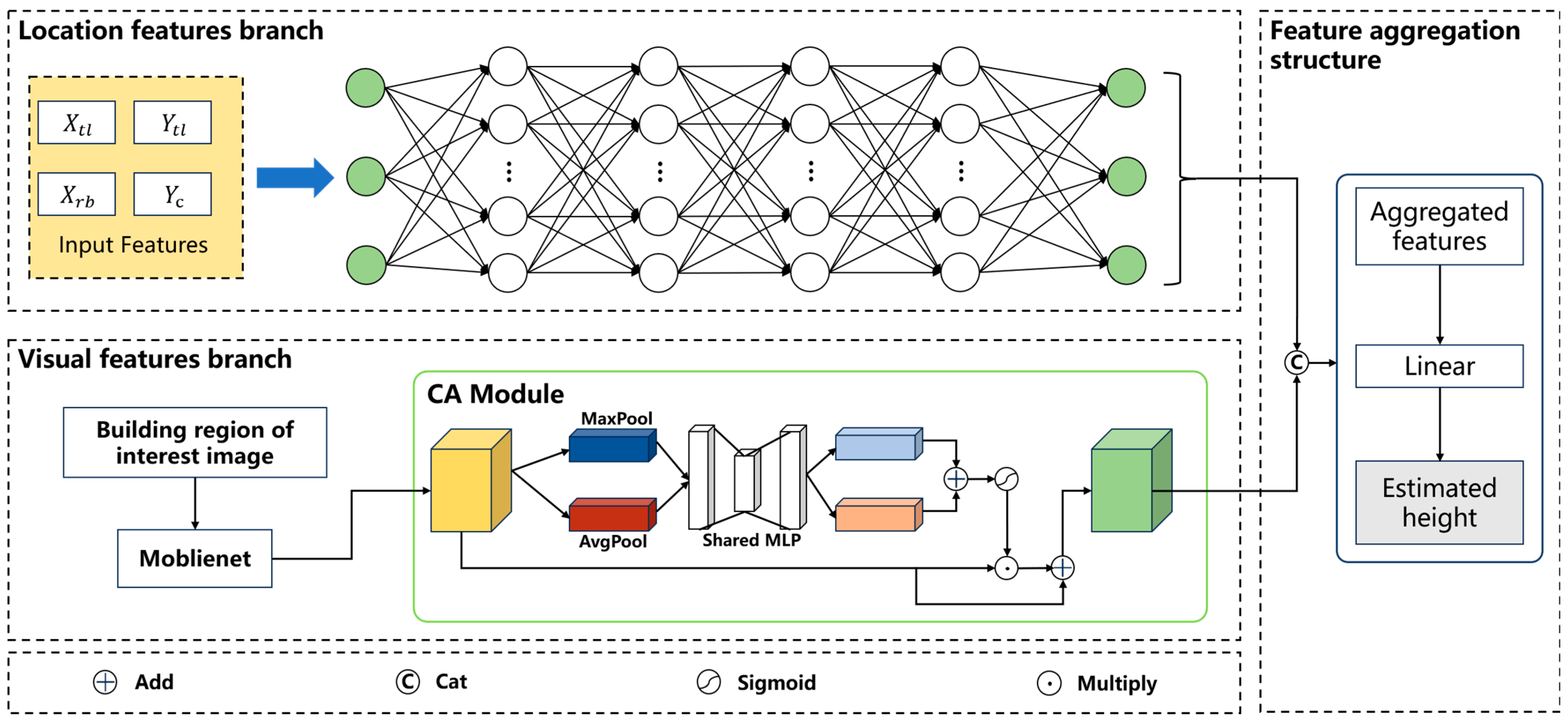
The proposed TBFF model consists of three parts: the location features branch, the building visual features branch, and the feature aggregation structure, as shown in Figure 6. Specifically, the location features branch takes the optimal location features identified through SHAP analysis as input data, and then uses a multilayer perception (MLP) to learn the implicit building height information.
The building visual features branch takes the region of interest image cropped by the bounding box of the extracted building as the independent input and uses a convolutional neural network (CNN) to extract higher-level intermediate visual information. The CNN used in this study is MobileNet, a lightweight network proposed by Google specifically to operate in environments with limited arithmetic resources [39,40]. In traditional neural networks, the importance of intermediate features is considered equivalent. Nevertheless, some features are often more important than others in practical applications, which can be achieved automatically using the attention mechanism. This allows the model to pay more attention to the important parts of the intermediate features, thereby improving its performance [41].
This study incorporated a channel attention mechanism [42,43] to enhance the importance of features across different channels in building region of interest images. The core of the channel attention mechanism is to utilize the global information of an image to dynamically adjust the weight of each channel. Firstly, the input feature map F undergoes average pooling and max pooling to generate the global features ( F a v g c and F m a x c ) of each channel. Then, a shared Multilayer Perceptron is applied to perform nonlinear mapping on the above global features, and the results are added to obtain the channel attention weights M C R C × 1 × 1 . Finally, the channel attention weights are multiplied by the input feature map to highlight the important channel features. The formula for channel attention is as follows:
M c = σ M L P A v g P o o l F + M L P M a x P o o l F
where σ represents the sigmoid function.
Subsequently, the features from the location feature branch and building visual feature branch are concatenated in the feature aggregation structure. Eventually, the output layer is a fully connected layer with one neuron, and its output represents the estimated height of the building.

2.3.4. Model Training and Evaluation

In deep learning, the initialization of model hyperparameters is particularly important [44]. The proper selection of hyperparameters can significantly enhance the model’s performance and training efficiency. The 1650 building samples were divided into training, validation, and test sets with a ratio of 8:1:1, where the validation set was used for model parameter optimization. In our study, the TBFF model was trained using the Adam optimizer [45] and mean squared error loss function. The specific settings of the model hyperparameters are presented in Table 2. The optimal batch size, learning rate, epoch, and hidden unit number identified through evaluation of the test set were 64, 0.0008, 200, and 64, respectively.
The model evaluation metrics include the root mean square error (RMSE), mean absolute error (MAE), and mean absolute percentage error (MAPE). The RMSE reflects the average deviation between the estimated value and the true value. The MAE reflects the reality of the error in the estimated value. The MAPE reflects the average relative deviation between the estimated and true values. The smaller the RMSE, MAE, and MAPE values, the more effective the regression model:
R M S E = 1 n i = 1 n ( y i y ^ i ) 2
M A E = 1 n i = 1 n y i y ^ i
M A P E = 1 n i = 1 n y i y ^ i y i
where n represents the number of building samples in the test set, y i represents the true value of the building height, y ^ i represents the estimated building height.

3. Results

3.1. Location Features Selection Results

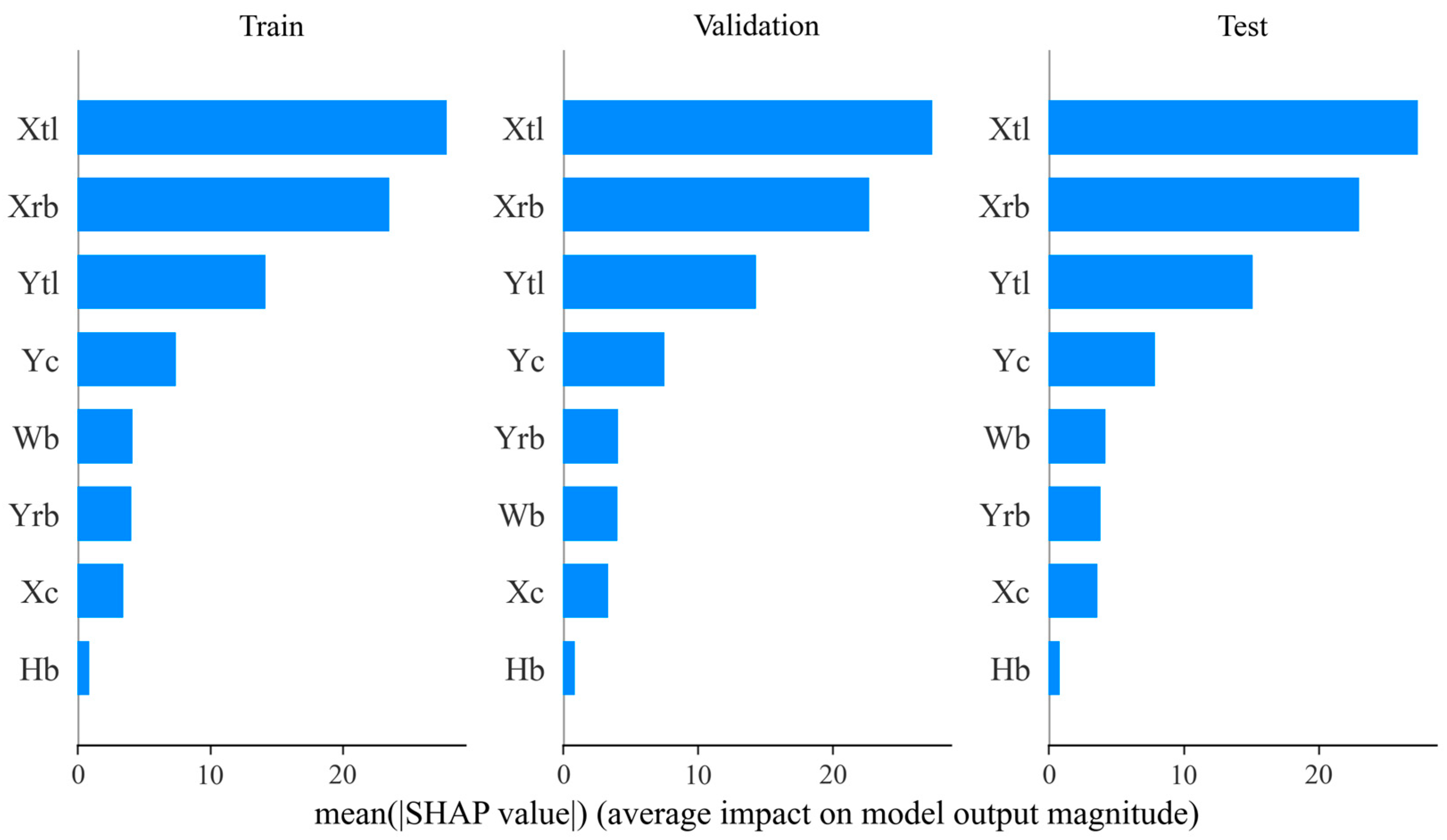
Firstly, we used all location features to train the MLP network, and the results obtained based on 5-fold cross-validation were RMSE 15.82 m, MAE 12.1 m, and MAPE 0.32. At the same time, to quantify the stability of the network, we used the Bootstrap sampling method to perform 1000 samplings on the test set and calculated the 95% confidence intervals of the RMSE and MAE. The specific values of the 95% confidence intervals are presented in Table 3. We calculated the SHAP values of all location features on the training, test, and validation sets and plotted the summary plot (Figure 7). The larger the SHAP value, the greater the influence of the feature on the building height estimation. Therefore, we took the features with SHAP values greater than 5 as important features, including Xtl, Xrb, Ytl, and Yc, and retrained the MLP network. The new MLP network trained with Xtl, Xrb, Ytl, and Yc has an RMSE of 16.83 m, an MAE of 13.23 m, and an MAPE of 0.33.
Although the building height estimation accuracy of the MLP network trained by Xtl, Xrb, Ytl, and Yc has decreased, the following experiments prove that the TBFF model can achieve the best building height estimation effects when the network is used as the location features branch of the TBFF model.

3.2. Ablation Study

In order to evaluate the contribution of each module to the performance of the TBFF model, we designed three ablation experiment configurations: retaining only the location feature branch, retaining only the visual feature branch, and the complete TBFF model. The evaluation metric values for each model are listed in Table 4. When the location features were Xtl, Xrb, Ytl, Yc, and the visual features branch used a channel attention mechanism, the TBFF model achieved the optimal estimation effect with an RMSE of 5.69 m, MAE of 3.97 m, and MAPE of 0.15. Compared with the location feature branch, when only the visual feature branch was used, the RMSE, MAE, and MAPE of the model were reduced by 59.77%, 64.7%, and 67.3%, respectively, indicating that the visual features are more important for height estimation. Compared with using all location features, when Xtl, Xrb, Ytl, and Yc were used as the input of the location features branch, the RMSE, MAE, and MAPE of the model were reduced by 11.23%, 11.97% and 6.25% respectively, indicating that it is reasonable to select Xtl, Xrb, Ytl, and Yc as important features. Compared with the location feature branch and the visual feature branch, the TBFF model has the smallest absolute and relative errors, indicating that the location features can help improve the model’s accuracy.
We present a scatter plot of the TBFF model’s estimated values and the ground truth (Figure 8a), along with the distribution of estimation errors (Figure 8b). As shown in Figure 8a, most of the scattered points cluster closely around the best-fit line, and the best-fit line significantly overlaps with the 1:1 reference line, indicating that the model is overall accurate. Moreover, a narrower confidence interval indicates that the TBFF model is stable. Locally, the TBFF model exhibited a tendency to overestimate the wind loads on low-rise buildings while underestimating those on high-rise buildings, indicating the presence of systematic bias and suggesting room for further improvement. In Figure 8b, the black dashed line represents the mean error, which is 0.05 m, indicating that the TBFF model exhibits a slight positive bias overall. The error distribution is bell-shaped and slightly right-skewed, with 71.88% of the estimation errors falling within a ±5 m range.
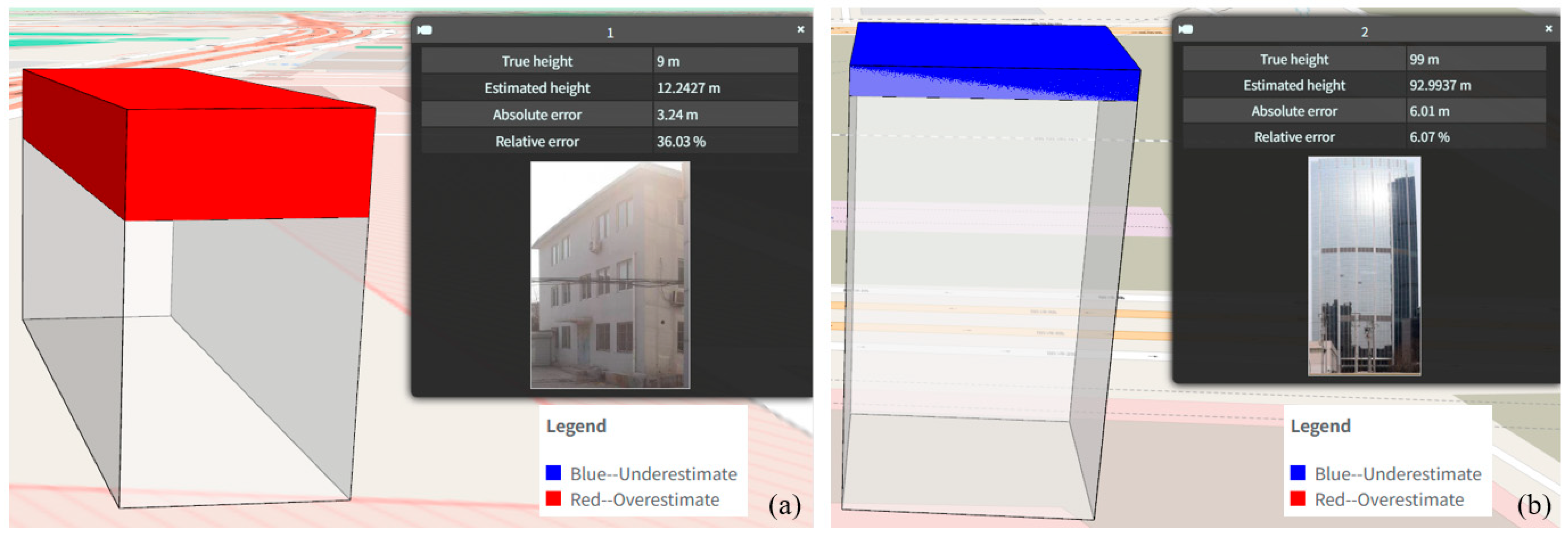
To investigate the phenomenon in which the TBFF model overestimates low-rise buildings and underestimates high-rise buildings, we selected two representative samples and constructed their LOD1 (level of detail 1) 3D building models using the Cesium visualization framework to visually demonstrate the estimation errors in a 3D scene. In Figure 9, red represents overestimation and blue represents underestimation. As shown in Figure 9a, the true height of the low-rise building is 9 m. Although the absolute error is only 3.24 m, the relative error amounts to 36.03% of the true height, which is unacceptable for low-rise buildings. As shown in Figure 9b, the true height of the high-rise building is 99 m. Although the absolute error is 6.01 m, the relative error is only 6.07% of the true height, which is acceptable for high-rise buildings. In the future, the TBFF model will focus on addressing the limitations of overestimating low-rise buildings.

4. Discussion

4.1. Location Features Importance Analysis

The quantitative analysis indicated the optimal location features combination for height estimation was Xtl, Xrb, Ytl, and Yc, and their shap values on the test set are 27.33, 22.99, 15.1, and 7.85, respectively. The shape values of Xtl and Xrb are greater than 20, indicating that the horizontal location features of the buildings in the panorama have a greater impact on the height estimation than the vertical position features. It may be surprising that building height, as a dependent variable in the vertical dimension, is more susceptible to vertical location features. Figure 10 shows the SHAP scatter plots of Xtl, Xrb, Ytl, and Yc to reveal the complex nonlinear relationship between the location features and height.
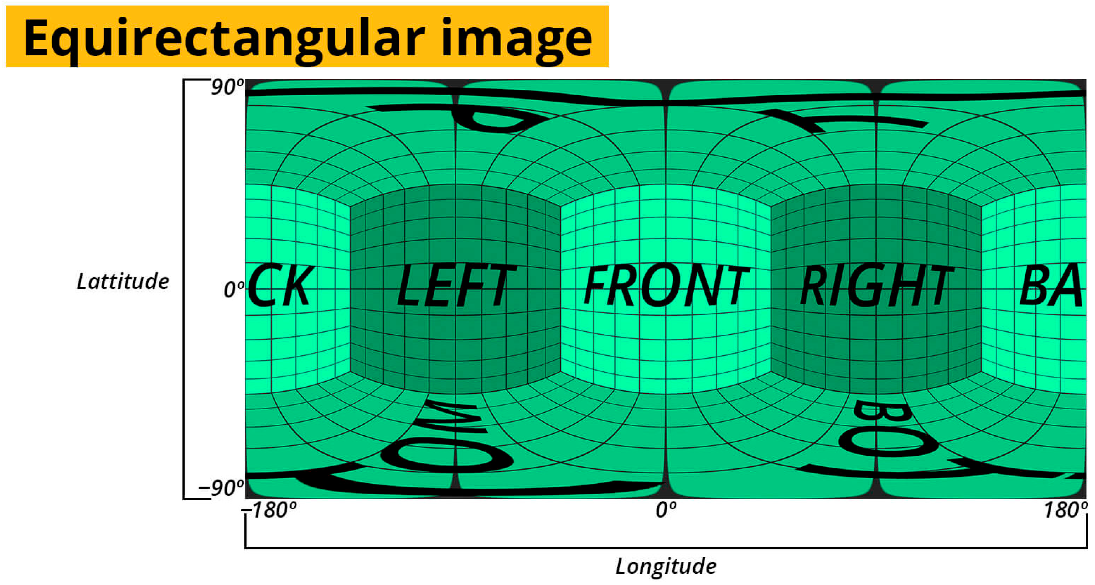
It can be seen that the influence of the two horizontal location features on the height is similar, where the effect of the feature on the height estimation experienced ranges from height underestimation to height overestimation. When the Xtl value and Xrb value are nearly 0.4, the SHAP values account for zero, indicating a better estimation without underestimation or overestimation. This signifies that the building height estimation will be better if the buildings’ horizontal locations are closer to the center of the street view image. Because the projection of the Baidu street view image is an equidistant cylindrical projection, which is characterized by the perpendicularity of the longitudinal and latitudinal lines to each other, the small degree of distortion in the center of the image can maintain a more realistic geometrical shape, and the edge of the stretching distortion is more obvious [46]. The Ytl vertical location feature pattern indicated that when the distance from the top of the building to the upper edge of the image is close to 0.23, the building height estimation will be more accurate. The Yc vertical location feature pattern indicated that the building height estimation is more accurate when the distance from the center of the building to the upper edge of the image is 0.37.
To make it easier to understand, we explain it using another projection method for panoramic images, the cube map projection. As shown in Figure 11, a panoramic image can be represented by the six faces of a cube (Top, Bottom, Front, Back, Left, Right), with the Top and Bottom faces exhibiting the most severe distortion. The distortion of the other four faces is relatively light, but within the four faces, the distortion at the center is 0, and the distortion increases as it approaches the face boundary. When the Xtl and Xrb values are 0.42, it indicates that the left and right boundaries of the building are close to the center of the Front face—i.e., the center of the building is close to the center of the panoramic image. In this case, image distortion is small and will not affect the height estimation. When the Ytl value is 0.23, the top of the building is located at the junction between the Top and Front faces. Since each face has a 90° × 90° field of view, the Front face spans 0.5 of the entire panorama in the vertical dimension, while the Top and Bottom faces each span 0.25. Moreover, since 0.23 is very close to 0.25, when the top of the building is located at the junction between the Top and Front faces, it will not affect height estimation. When the top of the building is located on the Top face—where distortion is especially severe—it positively enhances height estimation. Conversely, when the top of the building lies on one of the less distorted faces (Front, Back, Left, or Right), it negatively suppresses the height estimation. When the Yc value is 0.37, it does not affect the height estimation. In this case, the center of the building is located in the center of the upper half of the Front face, which is closer to the center of the panoramic image and has less image distortion. Theoretically, when the Yc value is 0.5, this feature does not affect the height estimation. We checked the sample data and found that the bases of all buildings were close to the center of the panoramic image in the vertical dimension. This implies that when the Yrb value is close to 0.5, it will not affect height estimation; therefore, the Yc value of 0.37 is reasonable. In other words, when the building lies in the upper half of the Front, Back, Left, or Right faces, the model can achieve a more accurate height estimation.
According to the pinhole camera model, the pixel height of an object in the image satisfies Equation (10), where himg is the object’s pixel height, f is the effective focal length, H is the object’s real-world height, and D is the distance between the object and the camera.
h i m g = f × H D
When the focal length is fixed, the distance becomes a critical factor in estimating the height of an object. Therefore, we applied a monocular depth estimation method to compute the depth values for the panoramic images, as shown in Figure 12. In the depth map, pixel colors near purple indicate that the point is closer to the camera, while colors closer to yellow indicate a greater distance from the camera. As shown in Figure 12, when the vertical pixel coordinate is fixed, changes in the horizontal pixel coordinate produce large variations in the depth values; that is, variations in the location features Xtl and Xrb lead to significant changes in distance. Moreover, Xtl and Xrb represent the horizontal orientation of the building, which implicitly conveys depth information. Therefore, in the building height estimation task, horizontal location features are more important than vertical location features.
Although the horizontal location features can indirectly represent the distance from the building to the camera, it may be better to directly use the distance from the building to the camera as a feature. Meanwhile, Che et al. [48] integrated building morphological features (area, perimeter, compactness, and fractality) with remote sensing features to estimate individual building heights, thereby demonstrating that morphological features are indeed useful for building height estimation. In the future, we will consider using building morphological features and the distance from the building to the camera to optimize the location-feature branch.

4.2. Comparison with Other Models

To evaluate the model’s effectiveness in height estimation, we compared the TBFF with the RF model proposed in [20] and the Pano2Geo model proposed in [21]. The RF model estimates the height of individual buildings by fusing 129 features from buildings, streets, and blocks. The Pano2Geo model uses the projection relationship between the two-dimensional image coordinate system and the spherical coordinate system and the three-dimensional space coordinate system to construct a conversion formula from two-dimensional pixel coordinates to three-dimensional geographic space coordinates. The building height is obtained by calculating the three-dimensional geographic space coordinates of the building height feature points in the panoramic image. The principle of Pano2Geo is shown in Figure 13, and the building height estimation formula is presented in Equation (11). It should be noted that only the Pano2Geo model was used for the comparison experiment, and other optimization strategies proposed by Fan et al. [21] were not adopted.
h b = tan p i t c h × d + h c
where h b represents the estimated building height, pitch represents the pitch angle between the highest point of the building and the center of the panoramic camera, d represents the distance from the building to the panoramic camera, and h c represents the panoramic camera height, which can be obtained from the DeviceHeight field in Baidu street view image metadata.
The pitch can be calculated from the building location feature Ytl, and the calculation formula is presented in Equation (12). The distance from the building to the camera can be calculated using the camera location and building geographic coordinates (Equation (13)). R represents the radius of the Earth, which is 6378 km. latA and latB represent the latitudes of points A and B on the Earth. lngA and lngB represent the longitudes of point A, point B on the earth.
p i t c h = 0.5 Y t l × 180
d = R   ×   arccos ( cos ( latA )   ×   cos ( latB )   ×   cos ( lngA lngB ) + sin ( latA )   ×   sin ( latB )
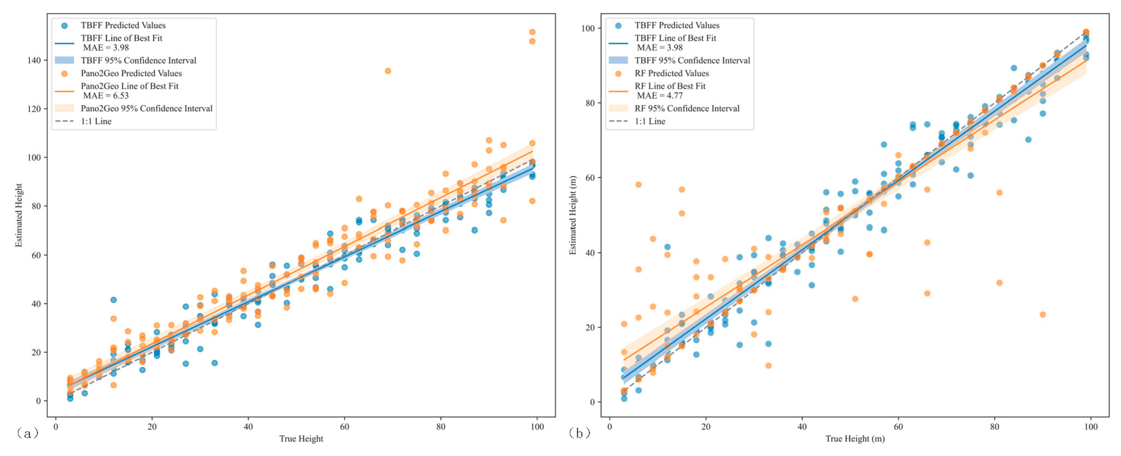
Fan et al. [21] used 45 buildings to evaluate the performance of their Pano2Geo model. Because we could not obtain these 45 building samples, we used our test set for comparison. The comparison results are presented in Table 5. It can be seen that the accuracy of the RF model is the worst, with RMSE of 10.83 m, MAE of 4.76 m, and MAPE of 0.32. The Pano2Geo model exhibited slightly better accuracy, with an RMSE of 10.51 m, MAE of 6.52 m, and MAPE of 0.22. Compared with RF, TBFF reduced RMSE by 51.9%, MAE by 16.59%, and MAPE by 53.12%. This indicates that the TBFF can significantly reduce extreme errors. Compared with Pano2Geo, TBFF achieved higher accuracy, with the RMSE reduced by 45.86%, MAE reduced by 39.11%, and MAPE reduced by 31.81%. Moreover, the upper bounds of the confidence intervals for RMSE and MAE in the TBFF are smaller than the lower bounds of those in Pano2Geo, indicating that the TBFF is more robust than Pano2Geo.
By drawing scatter plots between the estimated values and the true values of all models (Figure 14), the height estimation performance of each model is intuitively displayed. As shown in Figure 14a, the best-fit line of the Pano2Geo model lies above the 1:1 reference line, indicating that the Pano2Geo model exhibits a systematic bias and tends to overestimate building heights. In contrast, the best-fit line of the TBFF model aligns more closely with the 1:1 reference line, and its 95% confidence interval is tighter than that of the Pano2Geo model. As shown in Figure 14b, the RF model exhibits a greater deviation of its best-fit- line from the 1:1 reference line than the TBFF model, and its 95% confidence interval is also wider. These results underscore the effectiveness of the TBFF model in building height estimation tasks.
Although the Pano2Geo model can estimate building heights without training, the estimated height is not only affected by the variables pitch and d, but is also significantly affected by terrain undulations. The Pano2Geo model assumes that buildings and street-view image-capture vehicles are located at the same elevation. This assumption holds on flat terrain; however, when there are significant slope variations, it no longer applies, and the Pano2Geo model’s estimation error will increase. To address this issue, the Pano2Geo model must also incorporate DEM data. Although the RF model achieves a lower MAE, it tends to overestimate low-rise buildings and underestimate high-rise buildings, and its estimation errors are larger than those of the TBFF model. In contrast, the TBFF model can estimate building heights with high accuracy using only a single panoramic image after training, which demonstrates that it provides an efficient approach for height estimation from panoramas.

4.3. Features Uncertainty Analysis

To evaluate the robustness of the TBFF model under input feature perturbations, we employed Monte Carlo simulations to perform uncertainty analyses of the location and visual features. Specifically, random perturbations conforming to the empirical distributions of each feature type were injected, and the TBFF model was run independently 500 times to derive the probability distribution of the height estimation results. During the simulations, we adhered to the principle of controlled variables: when observing perturbations to the location features, the visual features remained unchanged; when observing perturbations to the visual features, the location features remained unchanged, ensuring that the analysis focused on the impact of each input feature level.
By drawing a frequency histogram of the coefficient of variation of the height estimation results, the effect of feature perturbations on the TBFF model output is visually demonstrated. In Monte Carlo simulations, the coefficient of variation (denoted as CV below) represents the relative uncertainty of the model outputs, and its calculation formula is given in Equation (14). The smaller the CV value, the more tightly clustered the model outputs are, indicating that the model is less affected by the feature perturbations.
C V = 1 n 1 i = 1 n y i y ¯ 2 y ¯
where n is the number of Monte Carlo simulations, y i is the model output from the i-th simulation, and y ¯ is the mean of the n simulation outputs.
From Figure 15, it can be seen that under location feature perturbations, the CV values for all samples are very small, with the vast majority of CV values close to zero. Across the entire test set, the mean CV was 0.0006, indicating that the TBFF model exhibits strong adaptability to variations in the location features.
To simulate visual feature perturbations, we added Gaussian noise to the building region of interest images, and Figure 16 shows its impact on the height prediction. From Figure 16, it can be observed that the CV follows a long-tail distribution, with most of the sample CV values concentrated between 0 and 0.05. Across the entire test set, the mean CV was 0.012, demonstrating that the TBFF is robust against perturbations in visual features. Compared to location feature perturbations, although visual feature perturbations increase the uncertainty of TBFF model predictions, this also indirectly indicates that building visual features are more important than location features for the height estimation task.
Overall, the TBFF model exhibits strong robustness and effectively withstands perturbations in both the location and visual features.

4.4. Practical Implications

Although the TBFF model shows high accuracy and robustness in building height estimation, its practical application value needs to be evaluated in combination with scenario requirements, such as urban planning. We also conducted a brief comparison between the street-view-based approach and other data acquisition methods in terms of effectiveness, cost, and reproducibility.
In the field of 3D city modeling, the OGC CityGML standard specifies that Level of Detail 1 (LOD1) models allow a certain margin of error in building height, with an error of ≤ 5m considered an acceptable threshold [49]. In our study, the TBFF model achieved an MAE of 3.97 m, which is below the threshold, demonstrating that it fully meets the data accuracy requirements for LOD1-level 3D city modeling. This result not only validates the practicality of the proposed method but also highlights the unique advantages of the street-view-based approach for low-cost 3D data production.
Table 6 presents the characteristics of the three methods for acquiring building height data. The table provides a systematic comparison of key performance indicators (spatial accuracy, coverage, update frequency, data cost, etc.) for street view imagery, UAV, and LiDAR in building height estimation. This reveals the advantages of the street-view-based approach in enabling the low-cost and rapid acquisition of building height data.

5. Conclusions

This study establishes a novel paradigm for cost-effective urban 3D information acquisition by achieving low-cost individual building-height estimation from panoramic street-view imagery. The key conclusions are as follows: the proposed TBFF model deeply integrates building location features with visual semantic features, achieving over 51% improvement in accuracy compared with similar methods, such as the RF model. The height estimation accuracy of the proposed method meets the OGC-defined LOD1 standard for 3D building modeling (height error ≤ 5 m), making it suitable for supporting applications such as urban planning, urban heat island simulation, disaster preparedness, and emergency response. SHAP analysis reveals that horizontal location features (such as the distance from the building to the camera) are key factors in height estimation, providing a theoretical basis for future model optimization. However, the model has certain limitations, such as overestimating the height of low-rise buildings and underestimating that of high-rise buildings. Addressing this issue will require an increase in the number of training samples to improve the prediction performance. Due to the distribution characteristics of street-view imagery, there are still blind spots in estimating the heights of non-roadside buildings. In future work, we plan to integrate multi-source satellite imagery and modern deep learning approaches to achieve comprehensive building height estimation across entire urban areas.

Author Contributions

Conceptualization, Shibo Ge, Jiping Liu and Xianghong Che; Data curation, Shibo Ge, Xianghong Che and Yong Wang; Formal analysis, Xianghong Che and Haosheng Huang; Funding acquisition, Jiping Liu and Yong Wang; Methodology, Shibo Ge, Jiping Liu and Xianghong Che; Project administration, Yong Wang; Supervision, Jiping Liu; Validation, Shibo Ge and Xianghong Che; Visualization, Shibo Ge; Writing—original draft, Shibo Ge; Writing—review & editing, Shibo Ge, Jiping Liu, Xianghong Che and Haosheng Huang. All authors have read and agreed to the published version of this manuscript.

Funding

This research study was funded by the National Key Research and Development Program of China [grant number 2022YFC3005705].

Data Availability Statement

The data used in this study are available from the Baidu Maps website: https://map.baidu.com/, (accessed on 22 October 2024).

Conflicts of Interest

The authors declare no conflicts of interest.

Abbreviations

The following abbreviations are used in this manuscript:
TBFFTwo-Branch feature fusion
SAMSegment Anything Model
MLPMulti-Layer Perceptron
FOVField of view
SARSynthetic aperture radar
ROIRegion of interest
LODLevel of Detail

References

  1. Biljecki, F.; Ledoux, H.; Stoter, J. Generating 3D city models without elevation data. Comput. Environ. Urban. Syst. 2017, 64, 1–18. [Google Scholar] [CrossRef]
  2. Chau, K.-W.; Wong, S.K.; Yau, Y.; Yeung, A. Determining optimal building height. Urban. Stud. 2007, 44, 591–607. [Google Scholar] [CrossRef]
  3. Khorshidi, S.; Carter, J.; Mohler, G.; Tita, G. Explaining crime diversity with google street view. J. Quant. Criminol. 2021, 37, 361–391. [Google Scholar] [CrossRef]
  4. Schug, F.; Frantz, D.; van der Linden, S.; Hostert, P. Gridded population mapping for Germany based on building density, height and type from Earth Observation data using census disaggregation and bottom-up estimates. PLoS ONE 2021, 16, e0249044. [Google Scholar] [CrossRef] [PubMed]
  5. Lee, T.; Kim, T. Automatic building height extraction by volumetric shadow analysis of monoscopic imagery. Int. J. Remote Sens. 2013, 34, 5834–5850. [Google Scholar] [CrossRef]
  6. Xu, W.; Feng, Z.; Wan, Q.; Xie, Y.; Feng, D.; Zhu, J.; Liu, Y. Building Height Extraction From High-Resolution Single-View Remote Sensing Images Using Shadow and Side Information. J. Sel. Top. Appl. Earth Observ. Remote Sens. 2024, 17, 6514–6528. [Google Scholar] [CrossRef]
  7. Zhang, C.; Cui, Y.; Zhu, Z.; Jiang, S.; Jiang, W. Building height extraction from GF-7 satellite images based on roof contour constrained stereo matching. Remote Sens. 2022, 14, 1566. [Google Scholar] [CrossRef]
  8. Guida, R.; Iodice, A.; Riccio, D. Height retrieval of isolated buildings from single high-resolution SAR images. Trans. Geosci. Remote Sens. 2010, 48, 2967–2979. [Google Scholar] [CrossRef]
  9. Lao, J.; Wang, C.; Zhu, X.; Xi, X.; Nie, S.; Wang, J.; Cheng, F.; Zhou, G. Retrieving building height in urban areas using ICESat-2 photon-counting LiDAR data. Int. J. Appl. Earth Obs. Geoinf. 2021, 104, 102596. [Google Scholar] [CrossRef]
  10. Shao, Y.; Taff, G.N.; Walsh, S.J. Shadow detection and building-height estimation using IKONOS data. Int. J. Remote Sens. 2011, 32, 6929–6944. [Google Scholar] [CrossRef]
  11. Sun, Y.; Shahzad, M.; Zhu, X.X. Building height estimation in single SAR image using OSM building footprints. In Proceedings of the 2017 Joint Urban Remote Sensing Event (JURSE), Dubai, United Arab Emirates, 6–8 March 2017; pp. 1–4. [Google Scholar] [CrossRef]
  12. Kim, H.; Han, S. Interactive 3D building modeling method using panoramic image sequences and digital map. Multimed. Tools Appl. 2018, 77, 27387–27404. [Google Scholar] [CrossRef]
  13. Biljecki, F.; Ito, K. Street view imagery in urban analytics and GIS: A review. Landsc. Urban. Plan. 2021, 215, 104217. [Google Scholar] [CrossRef]
  14. Long, Y.; Liu, L. How green are the streets? An analysis for central areas of Chinese cities using Tencent Street View. PLoS ONE 2017, 12, e0171110. [Google Scholar] [CrossRef] [PubMed]
  15. Feng, Y.; Chen, L.; He, X. Sky View Factor Calculation based on Baidu Street View Images and Its Application in Urban Heat Island Study. J. Geo-Inf. Sci. 2021, 23, 1998–2012. [Google Scholar]
  16. Zhao, Y.; Qi, J.; Zhang, R. Cbhe: Corner-based building height estimation for complex street scene images. In Proceedings of the World Wide Web Conference, San Francisco, CA, USA, 13–17 May 2019; pp. 2436–2447. [Google Scholar] [CrossRef]
  17. Al-Habashna, A.a. Building height estimation using street-view images, deep-learning, contour processing, and geospatial data. In Proceedings of the 2021 18th Conference on Robots and Vision (CRV), Burnaby, BC, Canada, 26–28 May 2021; pp. 103–110. [Google Scholar] [CrossRef]
  18. Díaz, E.; Arguello, H. An algorithm to estimate building heights from Google street-view imagery using single view metrology across a representational state transfer system. In Proceedings of the Dimensional Optical Metrology and Inspection for Practical Applications V, Baltimore, MD, USA, 16–17 April 2016; pp. 58–65. [Google Scholar] [CrossRef]
  19. Ureña-Pliego, M.; Martínez-Marín, R.; González-Rodrigo, B.; Marchamalo-Sacristán, M. Automatic building height estimation: Machine learning models for urban image analysis. Appl. Sci. 2023, 13, 5037. [Google Scholar] [CrossRef]
  20. Li, H.; Yuan, Z.; Dax, G.; Kong, G.; Fan, H.; Zipf, A.; Werner, M. Semi-Supervised Learning from Street-View Images and OpenStreetMap for Automatic Building Height Estimation. arXiv 2023, arXiv:2307.02574. [Google Scholar] [CrossRef]
  21. Fan, K.; Lin, A.; Wu, H.; Xu, Z. Pano2Geo: An efficient and robust building height estimation model using street-view panoramas. ISPRS-J. Photogramm. Remote Sens. 2024, 215, 177–191. [Google Scholar] [CrossRef]
  22. Ning, H.; Li, Z.; Ye, X.; Wang, S.; Wang, W.; Huang, X. Exploring the vertical dimension of street view image based on deep learning: A case study on lowest floor elevation estimation. Int. J. Geogr. Inf. Sci. 2022, 36, 1317–1342. [Google Scholar] [CrossRef]
  23. Ho, Y.-H.; Lee, C.-C.; Diaz, N.; Brody, S.; Mostafavi, A. Elev-vision: Automated lowest floor elevation estimation from segmenting street view images. ACM J. Comput. Sustain. Soc. 2024, 2, 1–18. [Google Scholar] [CrossRef]
  24. Ho, Y.-H.; Li, L.; Mostafavi, A. ELEV-VISION-SAM: Integrated Vision Language and Foundation Model for Automated Estimation of Building Lowest Floor Elevation. arXiv 2024, arXiv:2404.12606. [Google Scholar] [CrossRef]
  25. Available online: https://map.baidu.com/ (accessed on 22 October 2024).
  26. Kullback, S.; Leibler, R.A. On information and sufficiency. Ann. Math. Stat. 1951, 22, 79–86. [Google Scholar] [CrossRef]
  27. Yue, H.; Xie, H.; Liu, L.; Chen, J. Detecting people on the street and the streetscape physical environment from Baidu street view images and their effects on community-level street crime in a Chinese city. ISPRS Int. J. Geo-Inf. 2022, 11, 151. [Google Scholar] [CrossRef]
  28. Available online: https://en.wikipedia.org/wiki/List_of_street_view_services (accessed on 22 October 2024).
  29. Zhang, C.; Liu, L.; Cui, Y.; Huang, G.; Lin, W.; Yang, Y.; Hu, Y. A comprehensive survey on segment anything model for vision and beyond. arXiv 2023, arXiv:2305.08196. [Google Scholar] [CrossRef]
  30. Kirillov, A.; Mintun, E.; Ravi, N.; Mao, H.; Rolland, C.; Gustafson, L.; Xiao, T.; Whitehead, S.; Berg, A.C.; Lo, W.-Y. Segment anything. In Proceedings of the IEEE/CVF International Conference on Computer Vision, Paris, France, 1–6 October 2023; pp. 4015–4026. [Google Scholar] [CrossRef]
  31. Guyon, I.; Elisseeff, A. An introduction to variable and feature selection. J. Mach. Learn. Res. 2003, 3, 1157–1182. [Google Scholar] [CrossRef]
  32. Marcilio, W.E.; Eler, D.M. From explanations to feature selection: Assessing SHAP values as feature selection mechanism. In Proceedings of the 33rd SIBGRAPI Conference on Graphics, Patterns and Images (SIBGRAPI), Porto de Galinhas, Brazil, 7–10 November 2020. [Google Scholar] [CrossRef]
  33. Lundberg, S. A unified approach to interpreting model predictions. arXiv 2017, arXiv:1705.07874. [Google Scholar] [CrossRef]
  34. Zhang, J.; Ma, X.; Zhang, J.; Sun, D.; Zhou, X.; Mi, C.; Wen, H. Insights into geospatial heterogeneity of landslide susceptibility based on the SHAP-XGBoost model. J. Environ. Manag. 2023, 332, 117357. [Google Scholar] [CrossRef]
  35. Ekanayake, I.; Meddage, D.; Rathnayake, U. A novel approach to explain the black-box nature of machine learning in compressive strength predictions of concrete using Shapley additive explanations (SHAP). Case Stud. Constr. Mater. 2022, 16, e01059. [Google Scholar] [CrossRef]
  36. Nohara, Y.; Matsumoto, K.; Soejima, H.; Nakashima, N. Explanation of machine learning models using shapley additive explanation and application for real data in hospital. Comput. Meth. Programs Biomed. 2022, 214, 106584. [Google Scholar] [CrossRef]
  37. Ogawa, Y.; Oki, T.; Chen, S.; Sekimoto, Y. Joining street-view images and building footprint gis data. In Proceedings of the 1st ACM SIGSPATIAL International Workshop on Searching and Mining Large Collections of Geospatial Data, Beijing, China, 2 November 2021; pp. 18–24. [Google Scholar] [CrossRef]
  38. Kothuri, R.K.V.; Ravada, S.; Abugov, D. Quadtree and R-tree indexes in oracle spatial: A comparison using GIS data. In Proceedings of the 2002 ACM SIGMOD International Conference on Management of Data, Madison, WI, USA, 3–6 June 2002; pp. 546–557. [Google Scholar] [CrossRef]
  39. Sandler, M.; Howard, A.; Zhu, M.; Zhmoginov, A.; Chen, L.-C. Mobilenetv2: Inverted residuals and linear bottlenecks. In Proceedings of the IEEE Conference on Computer Vision and Pattern Recognition, Salt Lake City, UT, USA, 18–23 June 2018; pp. 4510–4520. [Google Scholar] [CrossRef]
  40. Howard, A.; Sandler, M.; Chu, G.; Chen, L.-C.; Chen, B.; Tan, M.; Wang, W.; Zhu, Y.; Pang, R.; Vasudevan, V. Searching for mobilenetv3. In Proceedings of the IEEE/CVF International Conference on Computer Vision, Seoul, Republic of Korea, 27–28 October 2019; pp. 1314–1324. [Google Scholar] [CrossRef]
  41. Guo, M.-H.; Xu, T.-X.; Liu, J.-J.; Liu, Z.-N.; Jiang, P.-T.; Mu, T.-J.; Zhang, S.-H.; Martin, R.R.; Cheng, M.-M.; Hu, S.-M. Attention mechanisms in computer vision: A survey. Comput. Vis. Media. 2022, 8, 331–368. [Google Scholar] [CrossRef]
  42. Hu, J.; Shen, L.; Sun, G. Squeeze-and-excitation networks. In Proceedings of the IEEE conference on Computer Vision and Pattern Recognition, Salt Lake City, UT, USA, 18–23 June 2018; pp. 7132–7141. [Google Scholar] [CrossRef]
  43. Woo, S.; Park, J.; Lee, J.-Y.; Kweon, I.S. Cbam: Convolutional block attention module. In Proceedings of the European Conference on Computer Vision (ECCV), Munich, Germany, 8–14 September 2018; pp. 3–19. [Google Scholar] [CrossRef]
  44. Xiao, X.; Yan, M.; Basodi, S.; Ji, C.; Pan, Y. Efficient hyperparameter optimization in deep learning using a variable length genetic algorithm. arXiv 2020, arXiv:2006.12703. [Google Scholar] [CrossRef]
  45. Kingma, D.P. Adam: A method for stochastic optimization. arXiv 2014, arXiv:1412.6980. [Google Scholar] [CrossRef]
  46. Yang, B. A mathematical investigation on the distance-preserving property of an equidistant cylindrical projection. arXiv 2021, arXiv:2101.03972. [Google Scholar] [CrossRef]
  47. Available online: https://stateofvr.com/1_the-basics.html (accessed on 7 May 2025).
  48. Che, Y.; Li, X.; Liu, X.; Wang, Y.; Liao, W.; Zheng, X.; Zhang, X.; Xu, X.; Shi, Q.; Zhu, J. 3D-GloBFP: The first global three-dimensional building footprint dataset. Earth Syst. Sci. Data Discuss. 2024, 16, 5357–5374. [Google Scholar] [CrossRef]
  49. Available online: https://portal.ogc.org/files/?artifact_id=33758 (accessed on 11 July 2025).
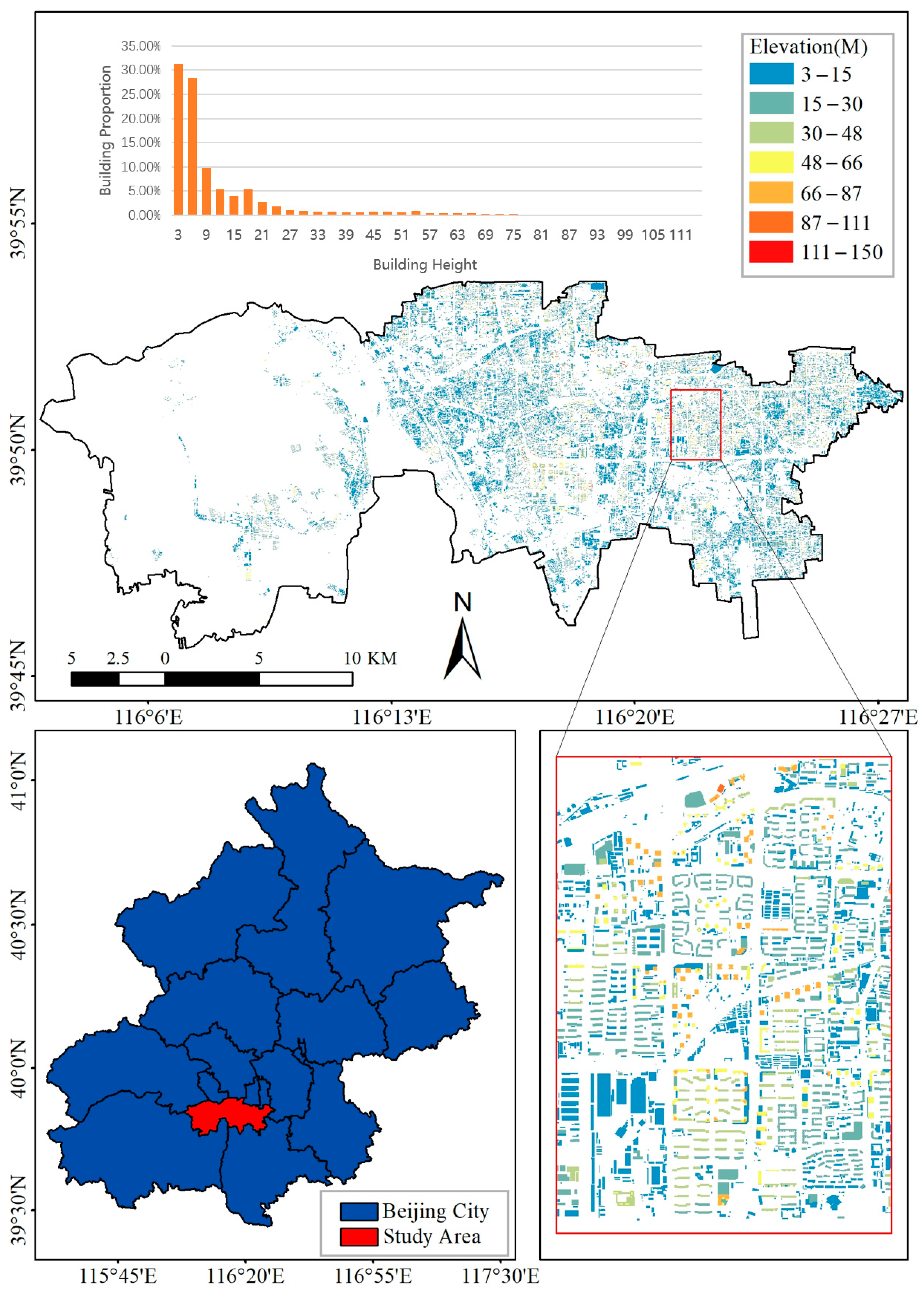
Figure 1. Study area.
Ijgi 14 00297 g001
Figure 2. Overall framework of the proposed method.
Ijgi 14 00297 g002
Figure 3. Building location feature illustration.
Ijgi 14 00297 g003
Figure 4. Algorithmic flow for cross-view matching of buildings. Heading represents the forward direction of the street view capture vehicle.
Ijgi 14 00297 g004
Figure 5. Horizontal azimuth relationship.
Ijgi 14 00297 g005
Figure 6. Two-branch feature fusion network architecture.
Ijgi 14 00297 g006
Figure 7. Location feature summary plot.
Ijgi 14 00297 g007
Figure 8. (a) Scatterplot of the estimated and true building heights; (b) frequency of the height errors.
Ijgi 14 00297 g008
Figure 9. (a) Overestimation of low-rise buildings; (b) Underestimation of high-rise buildings.
Ijgi 14 00297 g009
Figure 10. Distribution of SHAP values for the optimal four location features (red lines indicate a LOWESS fitting curve).
Ijgi 14 00297 g010
Figure 11. Schematic diagram of panoramic image distortion [47].
Ijgi 14 00297 g011
Figure 12. Panoramic depth map.
Ijgi 14 00297 g012
Figure 13. Schematic of the Pano2Geo model.
Ijgi 14 00297 g013
Figure 14. (a) TBFF vs. Pano2Geo estimation error scatter diagram; (b) TBFF vs. RF estimation error scatter diagram.
Ijgi 14 00297 g014
Figure 15. Coefficient of variation frequency histogram of the height estimation results under location feature perturbations.
Ijgi 14 00297 g015
Figure 16. Coefficient of variation frequency histogram of the height estimation results under visual feature perturbations.
Ijgi 14 00297 g016
Table 1. Building-height estimation method in street-view imagery.
Image TypeMedthodReferences
PerspectiveSingle view geometryZhao et al. [16]
Al-Habashna [17]
Díaz & Arguello [18]
Proportional relationshipUreña-Pliego [19]
Multimodal feature fusionLi et al. [20]
PanoramicSingle view geometryFan et al. [21]
Ning et al. [22]
Ho et al. [23]
Ho et al. [24]
Table 2. Model hyperparameter settings.
HyperparametersDescriptionInitial ValueOptimal Value
Batch sizeThe number of samples input into the model each time8, 16, 32, 64, 12864
Learning rateThe step size for parameter updates based on gradients during each iteration0.00001, 0.0001, 0.0010.0008
EpochThe number of training iterations100, 150, 200, 250200
Hidden unit numberThe number of neurons in the hidden layer of the location features branch16, 32, 6464
Table 3. Comparison of different combinations of location features.
NoLocation FeaturesRMSE (95% CI)MAE (95% CI)MAPE
1all features15.82 [13.98, 17.70]12.10 [10.60, 13.60]0.41
2Xtl, Xrb,
Ytl, Yc
16.83 [14.88, 18.71]13.23 [11.68, 14.88]0.52
Table 4. Comparison of the different models.
No Fusion Type RMSE (95% CI) MAE (95% CI) MAPE
1Location features branch
(Xtl, Xrb, Ytl, Yc)
16.83 [14.88, 18.71]13.23 [11.68, 14.88]0.52
2Visual features branch
(MoblienetV2 + Channel Attention)
6.77 [5.48, 8.27]4.67 [3.98, 5.48]0.17
3TBFF (all location features)6.41 [5.23, 7.73]4.51 [3.87, 5.28]0.16
4TBFF (Xtl, Xrb, Ytl, Yc)5.69 [4.69, 6.88]3.97 [3.40, 4.65]0.15
Table 5. Estimation metrics comparison between the TBFF and Pano2Geo models.
NoModelRMSE (95% CI)MAE (95% CI)MAPE
1Pano2Geo10.51 [7.04, 13.79]6.52 [5.33, 7.97]0.22
2RF11.83 [8.52, 15.09]4.76 [3.28, 6.54]0.32
3TBFF5.69 [4.69, 6.88]3.97 [3.40, 4.65]0.15
Table 6. Comparison of multi-source building height acquisition methods.
DimensionsStreet View ImageryOblique UAV PhotogrammetryAirborne LiDAR
Spatial accuracyMeter levelCentimeter levelCentimeter level
CoverageAlong streetsLocal (task planning)Local (cost-limited)
Update frequencyHigh (depends on map vendor updates)Medium (active collection required)Low (cost-limited)
Data costsLow (public API)Medium (equipment + manpower)High
Applicable scenariosHeight quick estimateFine-scale modeling of target objectsHigh precision requirements
Disclaimer/Publisher’s Note: The statements, opinions and data contained in all publications are solely those of the individual author(s) and contributor(s) and not of MDPI and/or the editor(s). MDPI and/or the editor(s) disclaim responsibility for any injury to people or property resulting from any ideas, methods, instructions or products referred to in the content.