Article

A Reversible Compression Coding Method for 3D Property Volumes

1
Research Institute for Smart Cities, School of Architecture and Urban Planning, Shenzhen University, Shenzhen 518060, China
2
School of Resource and Environmental Sciences, Wuhan University, Wuhan 430079, China
3
Shenzhen Data Management Center of Planning and Natural Resources, Shenzhen 518060, China
4
Key Laboratory of Digital Mapping and Land Information Application, Ministry of Natural Resources, Wuhan 430079, China
5
Shenzhen Key Laboratory of Digital Twin Technologies for Cities, Shenzhen 518060, China
6
Guangdong–Hong Kong-Macau Joint Laboratory for Smart Cities, Shenzhen 518060, China
7
MNR Key Laboratory of Urban Land Resources Monitoring and Simulation, Shenzhen 518060, China
8
State Key Laboratory of Subtropical Building and Urban Science, Shenzhen 518060, China
*
Author to whom correspondence should be addressed.
ISPRS Int. J. Geo-Inf. 2025, 14(7), 263; https://doi.org/10.3390/ijgi14070263
Submission received: 2 May 2025 / Revised: 25 June 2025 / Accepted: 3 July 2025 / Published: 5 July 2025

Abstract

3D (three-dimensional) property volume is an important data carrier for 3D land administration by using 3D cadastral technology, which can be used to express the legal space (property rights) scope matching with physical entities such as buildings and land. A 3D property volume is represented by a dense set of 3D coordinate points arranged in a predefined order and is displayed alongside the parcel map for reference and utilization by readers. To store a 3D property volume in the database, it is essential to record the connectivity relationships among the original 3D coordinate points, the associations between points and lines for representing boundary lines, and the relationships between lines for defining surfaces. Only by preserving the data structure that represents the relationships among points, lines, and surfaces can the 3D property volume in a parcel map be fully reconstructed. This approach inevitably results in the database storage volume significantly exceeding the original size of the point set, thereby causing storage redundancy. Consequently, this paper introduces a reversible 3D property volume compression coding method (called 3DPV-CC) to address this issue. By analyzing the distribution characteristics of the coordinate points of the 3D property volume, a specific rule for sorting the coordinate points is designed, enabling the database to have the ability of data storage and recovery by merely storing a reordered point set. The experimental results show that the 3DPV-CC method has excellent support capabilities for 3D property volumes of the vertical and slopped types, and can compress and restore the coordinate point set of the 3D property volume for drawing 3D parcel maps. The compression capacity of our method in the test is between 23.66% and 38.42%, higher than the general data compression methods (ZIP/7Z/RAR: 8.37–10.32%). By means of this method, land or real estate administrators from government departments can store 3D property volume data at a lower cost. This is conducive to enhancing the informatization level of land management.

1. Introduction

With the acceleration of global urbanization and the increase in population density, the use and management of land space have transitioned from planar to more complex three-dimensional structures. By integrating multiple dimensions of land management functions, the establishment of a comprehensive 3D land management system has emerged as a crucial trend in contemporary land spatial information management [1,2]. Ownership registration remains a fundamental and critical component of land management. To ensure that land ownership is clearly defined and to avoid property rights disputes caused by ambiguous boundaries or neighbor relations, the land management system generates a legally valid ownership certificate for each landowner or user, along with a land use scope map featuring clear boundaries to secure the ownership of land and real estate [3,4]. A 3D property volume acts as the primary carrier employed to express the spatial property rights scope within a land management system in 3D manners, precisely depicting the geometric shape, the topological relationships and the spatial structure [5]. The basis of a 3D property volume is a set of points. For the point sets to effectively represent the structure of a 3D property volume in 3D parcel maps, topological relationships must be preserved (It serves to maintain the definition of property rights, data consistency in 3D land [6], 3D spatial analysis and proximity queries [7], as well as the segmentation and merging of 3D property volumes during the land management process [8]). Consequently, it is necessary to integrate at least three types of data tables (point, line, and surface) within the database. The point table is utilized to store the 3D coordinates of each boundary point. The line table records the connectivity between pairs of points. The surface table documents the connections of lines, and the orientations of each face required for constructing a 3D interface. Obviously, once the data content of a 3D property volume is incorporated into the database, its data volume significantly increases (at least two new tables are required to record the topological relationships between geometric elements).
As illustrated in Figure 1, this 3D property volume represents the underground land use range of the Guomao Subway Station in Shenzhen, which comprises 632 3D coordinate points. When these coordinate points are stored in the database, it is essential to create a line table and a surface table to preserve the connectivity relationships between points (lines) and the relationships between lines that form surfaces, thereby ensuring accurate description and reconstruction of the shapes.
The 3D property volume is frequently employed to describe building space [9], and its boundaries are typically regular—either parallel or perpendicular to the ground. Only a limited number of boundary faces are inclined, thereby forming two types of property volumes with distinct morphological characteristics in our paper. During the construction of 3D volumes through the combination of points, lines, and surfaces, coordinate points can be systematically reordered in a structured manner. This eliminates the need to record line and surface tables in the database, as the point set can be reconstructed into the required 3D structure within the 3D parcel map. The method of compressing and encoding all boundary point coordinates of complex 3D property volumes is referred to as a reversible compression coding method for 3D property volumes, called the 3DPV-CC solution. The encoding process maintains the integrity of the topological structure and enables the recovery of the coordinate sequence set, effectively addressing the issue of redundant database storage for 3D property volumes.
The sections of this paper are organized as follows: The first section serves as the introduction, where we discuss the problems to be addressed and the significance of this research. Section 2 provides a summary of related research on this issue. In the third section, we present the implementation process of the 3DPV-CC solution. Section 3 describes each detail of the method flow. Section 4 includes experiments conducted using real data to verify both compression effectiveness and reduction effects. Finally, in Section 5, we provide a summary and outlook.

2. Related Works

The related work presented in this paper encompasses the development of 3D property volumes and the compression of 3D spatial models.

2.1. 3D Property Volume

In the context of 3D land administration systems, the concept of 3D property volume is introduced as a 3D model for representing property rights space (legal space), typically stored within spatial databases [10]. The geometric structure is constructed using real 3D coordinate points on the Earth obtained through field surveying. This structure forms a topological model composed of vertices (a kind of point representing graphical topology), edges (a kind of line representing graphical topology), and surfaces, which altogether facilitate the computation, querying, and analysis of cadastral information [11]. In order to achieve the data organization of 3D property volumes, various model structures can be employed. For instance, by employing Construction Solid Geometry (CSG) modeling, complex spatial features can be represented through the Boolean operations and combinations of various basic geometric primitives, resulting in a water-tight model [12]. This method is especially well-suited for symmetric geometric structures. Boundary Representation (B-Rep) constructs a model by defining the boundary of an object through elements such as faces, edges, and vertices, which collectively delineate the geometric form of the object [13]. This method is particularly well-suited for scenarios that demand precise processing of boundary details and irregular shapes, characteristics frequently encountered in the structural organization of 3D property volume models. In addition, Sweep Representations generate 3D structures by moving 2D sections along characteristic paths, making them particularly suitable for regular architecture-shaped 3D property volumes [14]. This model is essentially a parameterized structure, facilitating batch generation. In the research of 3D property volumes, some scholars have argued that the model structure of 3D property volumes is contingent upon the shape of the corresponding physical objects. For instance, these structures may include 3D prism space units represented by 2D graphics, design format space units (2D + Text Description), semi-open space units, polygon slice space units, single-value step space units, multi-value step space units, and conventional 3D space units [15,16] (Figure 2). For instance, woodlands and grasslands are typically categorized as semi-open space units; complex building spaces, on the other hand, are represented using either single-value step space units or multi-value step space units, depending on their structural complexity [17].
A 3D property volume Is a specific 3D spatial model characterized by Its physical shapes or corresponding geometric attributes. Implementing rule-driven structural compression is essential for minimizing its storage requirements in the database. Regardless of whether the Sweep, CSG, or B-Rep method is employed to construct the model, none of these methods fully capture the unique features of the model.

2.2. Compressing a 3D Property Volume

The 3D property volume structure encompasses geometric elements such as points, lines, and surfaces, as well as topological information including nodes, boundaries, and surfaces. When the information is intact, the 3D property volume can either be stored in a database or reconstructed into a 3D model with visualization capabilities from the database. Consequently, the process of model compression must consider both geometric and topological aspects concurrently to ensure a comprehensive optimization.
Early compression algorithms for 3D models focused on terrain data represented by triangle meshes, where each triangle shared two vertices during the recording process. To address this, Deering introduced a mesh compression method that organized triangle points in grid order to minimize vertex coding redundancy [18]. Building upon Deering’s work, Bajaj [19] further enhanced the mesh compression technique by incorporating hierarchical representations to satisfy the storage and processing demands of large-scale 3D datasets. At its core, this approach uses a queue to record the topological ordering of point sets, enabling efficient modifications to triangular mesh format models. In 2017, Janečka [20] proposed a parallelogram prediction method based on an edge disconnection algorithm. This method first records the connectivity information between points and subsequently marks other geometric details sequentially to ensure the fidelity of the geometric structure. Terrain triangulation is a classical 3D modeling structure characterized by its simple surface geometry. Compression of terrain triangulation primarily focuses on the contextual connectivity of triangular facets.
Complex model structures often consist of more than one undulating mesh, comprising multiple closed surfaces, also referred to as sub-meshes or parts. These meshes can either be treated as a single object or as multiple distinct objects. In 2013, Gurung [21] introduced a compact connectivity representation method (called Zipper) that reduces storage requirements by constructing an approximate Hamiltonian cycle to simulate the point set structure within a single mesh. In the Zipper method, the database stores the difference values of the mesh point sets rather than the absolute coordinates and connection relationships of all points. However, this approach still necessitates additional data tables to store triangular face relationships. Siddeq [22] proposed a method for compressing geometry and connectivity while preserving the number of vertices and the relationships between point sets forming triangular faces. In this method, each vertex is first encoded as a value, and then the positional difference between two adjacent vertices is differentially encoded to represent triangular faces. For non-manifold meshes, which may consist of multiple meshes, Nguyen et al. [23] performed lossless “point-to-edge” compression on each mesh, achieving higher compression ratios compared to common file compression methods such as Gzip. Without considering topological relationships, model compression techniques can directly deduplicate and encode the coordinates of the point sets that constitute the model, thereby reducing its size. Nevertheless, these approaches risk losing the internal spatial structure relationships within the model.
In recent years, the storage and compression of structural relationships in models have attracted considerable scholarly attention. Wei et al. [24] proposed a voxel-based chain code representation method for 3D models. This approach systematically organizes triangular facets according to the chain code structure, thereby achieving facet-level compression of 3D models. This technique essentially refines the traditional chain data structure. Li et al. [25] demonstrated that feature preservation can be effectively incorporated into model compression strategies. In 2021, they utilized local mesh smoothness and plane operators to perform segment-by-segment matching compression on chain triangulations for urban architectural meshes. This method not only simplifies the model but also preserves the integrity of the architectural structure.
Further on, Lin et al. [26] introduced a quadrilateral organization method with an implicit chain structure. This approach preserved the mesh characteristics through vertex optimization and achieved high reconstruction accuracy and mesh quality using only a minimal count of vertices. However, while chain-based compression coding can effectively simplify models, it requires modifying the number of vertices and facets in the model, which may alter its topological structure. Moreover, with advancements in deep learning technology, 3D model compression techniques have begun to diverge from traditional compression algorithms. For instance, in the deep learning-based lossless compression method for triangular meshes proposed by Zhao et al. [27], the inclusion of deep connectivity prediction values in the learning function reduces redundant geometric information in 3D models while maintaining block connectivity. Nevertheless, the original shape of the model cannot be fully recovered post-compression. To address this issue, Wang [28] developed an implicit 3D reconstruction technique based on deep learning that alternately transforms the latent topological representation of point clouds and meshes to enhance detail recovery. In 2024, Balreira [29] employed a lossless compression algorithm based on upper triangular matrices to efficiently encode the connectivity information of 3D meshes, reducing storage and transmission complexity through unique edge encoding.
Based on the current research progress, it is evident that a 3D property volume is essentially a 3D data model with distinct morphological characteristics. However, existing 3D model compression algorithms may encounter the following challenges when addressing the compression of 3D property volumes: (1) insufficient consideration of the shape characteristics of 3D properties; (2) difficulty in simultaneously preserving geometric and topological information; (3) ensuring the recoverability of the compressed model. These issues collectively contribute to the complexity of achieving efficient compressed representation of 3D property volumes within databases.

3. Methodology

3.1. The Context of the 3DPV-CC Solution

Modern 3D cadastral maps are typically stored in databases and frequently require printing as paper maps for practical use. The 3D property volume, as the most critical expression element of a 3D cadastre, consists of a series of point sets with a defined spatial structure. To achieve efficient recording and visualization of 3D property by converting 3D property volumes between databases and 3D cadastral drawings at minimal storage cost, we propose a compression coding algorithm for continuous coordinate strings of 3D property volumes. This algorithm ensures precise restoration of the 3D property volumes while maintaining its geometric structure and topological relationships, thereby enabling the limited layout space to effectively accommodate the display of 3D property information.
We designate the method proposed in this paper as the 3DPV-CC method. By reducing the dimensionality of the representation of the 3D property volume model, it facilitates the bidirectional conversion between the 3D boundary point sequence in the database and the 3D property volume model, requiring only the storage of the point set table. A detailed process description involving the classifier, encoder, decoder, inpainting, and visualization is presented in Figure 3. First, the Classifier categorized the input 3D property volume into vertical and slope types. Subsequently, the Encoder encoded these two types separately, enabling them to be stored in the database with a reduced data volume (specific point sequence). Finally, the Decoder was employed to restore the point sequence in the database to the original 3D model. During this process, we analyzed the effects of the encoding and decoding results.

3.2. Classifier

According to the morphological structure of the 3D property volume, we categorize it into two types: Wall-Vertical Property Volume and Wall-Slopping Property Volume. This classification aligns with the framework proposed by Thompson et al. [15,16] (See Section 2.1). Specifically, based on the structural characteristics of the model, types 3, 4, 5, and 6 of the seven types correspond to the vertical wall category, while type 7 corresponds to the slopped wall category.
The Wall-Vertical Property Volume represents a three-dimensional model distinguished by its simple and symmetrical geometric characteristics. This type of model typically comprises vertical facades with predominantly horizontal top and bottom surfaces, while the sides remain perpendicular to the base. Furthermore, all adjacent faces of a Wall-Vertical Property Volume exhibit vertical relationships. Such volumes encompass standardized building units, including residential buildings, office buildings, and land plots, which generally feature vertical facades and demonstrate a relatively organized structural layout. Due to their representation of standardized building units, Wall-Vertical Property Volumes are widely applied in urban planning, land resource management, and property rights demarcation. The geometric and topological information associated with these volumes can be analyzed and stored in a standardized and systematic manner, facilitating efficient data processing and management.
The Wall-Sloping Property Volume model refers to a 3D property volume characterized by complex geometry, asymmetric structures, and the absence of standard vertical facades. This type of model commonly occurs in buildings or parcels with intricate shapes, such as historical structures, irregular constructions, and specially designed modern buildings. The surfaces of these models often feature diverse concave and convex shapes or curved surfaces, which significantly increase the complexity of spatial geometric relationships and render boundaries no longer confined to traditional lines or planes. Consequently, Wall-Sloping Property Volume present greater challenges in terms of representation and encoding. In this paper, irregular models are categorized into two types: convex and concave. Convex models are defined by all adjacent faces forming angles less than 180 degrees, whereas concave models include angles exceeding 180 degrees.

3.3. Encoder

The primary function of the model encoder is to transform the complex 3D property volume into an ordered list of boundary points. A continuous boundary point list serves as an effective representation of geometric information, including boundary points, edges, and surfaces. This approach allows for the storage of geometric shapes and spatial relationships of the property volume in a simplified data structure while preserving the topological information necessary for reconstructing the 3D model.

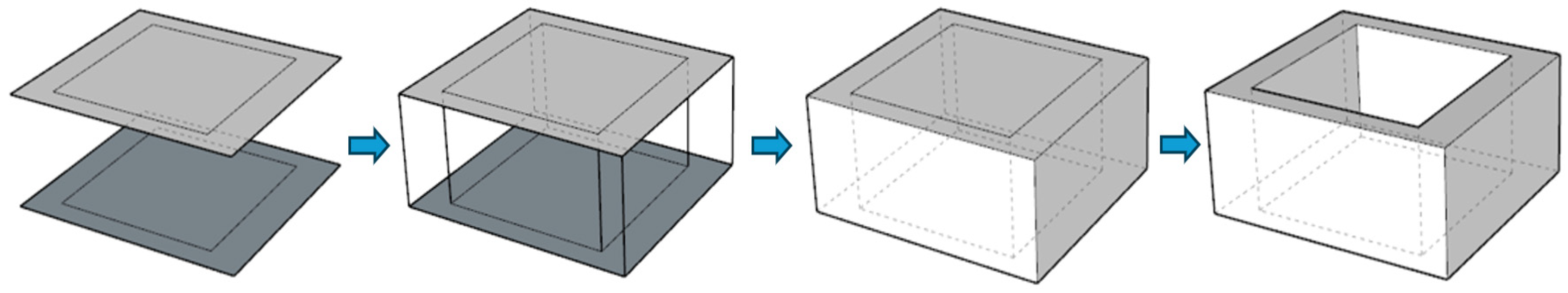
3.3.1. Vertical Type Encoder

The coding of the Wall-Vertical Property Volume model employs a grouping strategy, which divides the surface in the model into multiple groups. Each group contains continuous non-vertical planes, and the point sets within these non-vertical planes are recorded in a specified order (either clockwise or counterclockwise) to form a sequence point set. The sequence point sets of each group are then concatenated end-to-end for storage. Taking Figure 4 as an example, the 3D property volume is divided into two groups of point sets (outer wall surface and inner wall surface), with the point sets recorded in right-handed (clockwise) order.
The pseudo-code of the encoding algorithm of the Wall-Vertical Property Volume is presented in Figure 5. In this algorithm, we define the variable NVF to represent the non-vertical faces within the model. The variable PF denotes the last traversed face, while TF is utilized to store points located on the horizontal plane of the current point. The variable CV is employed to store the currently traversed vertices, and the variable NTA is used to record the vertices of the model that have yet to be traversed. Additionally, the variable VA is introduced to store the subsequent vertex sequence. Through the execution of the algorithm, the resulting VA represents a set of rearranged points that effectively preserve the equivalence to the original 3D property volume.

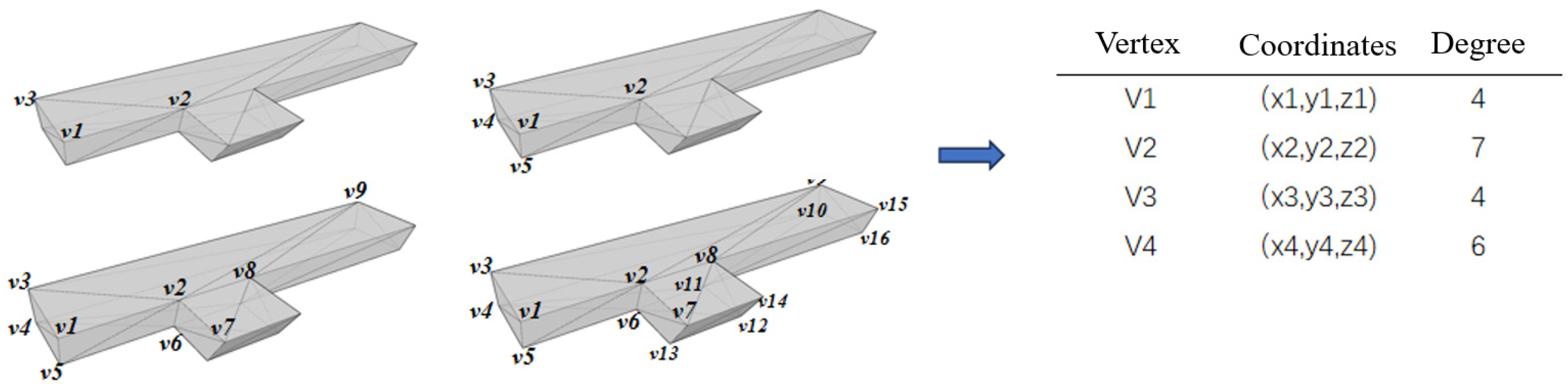
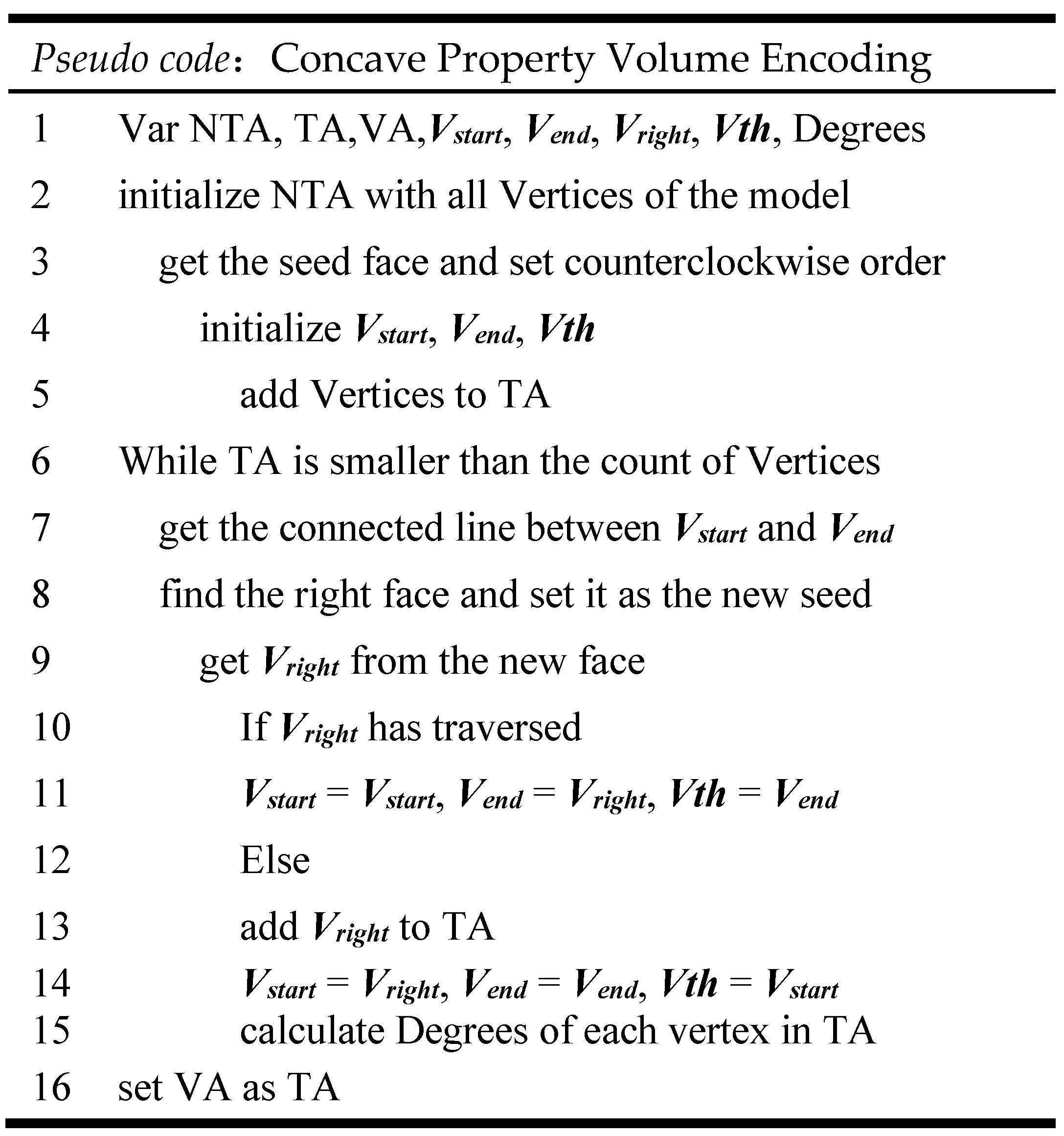
3.3.2. Slopping Type Encoder
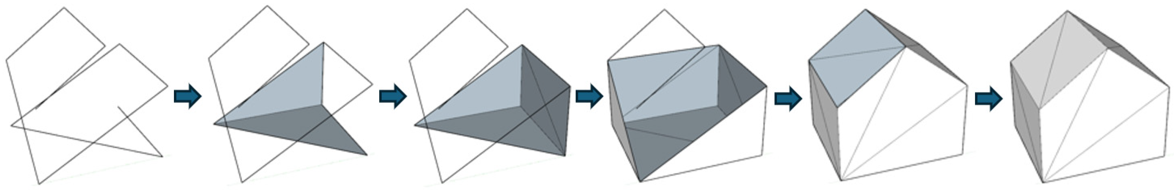
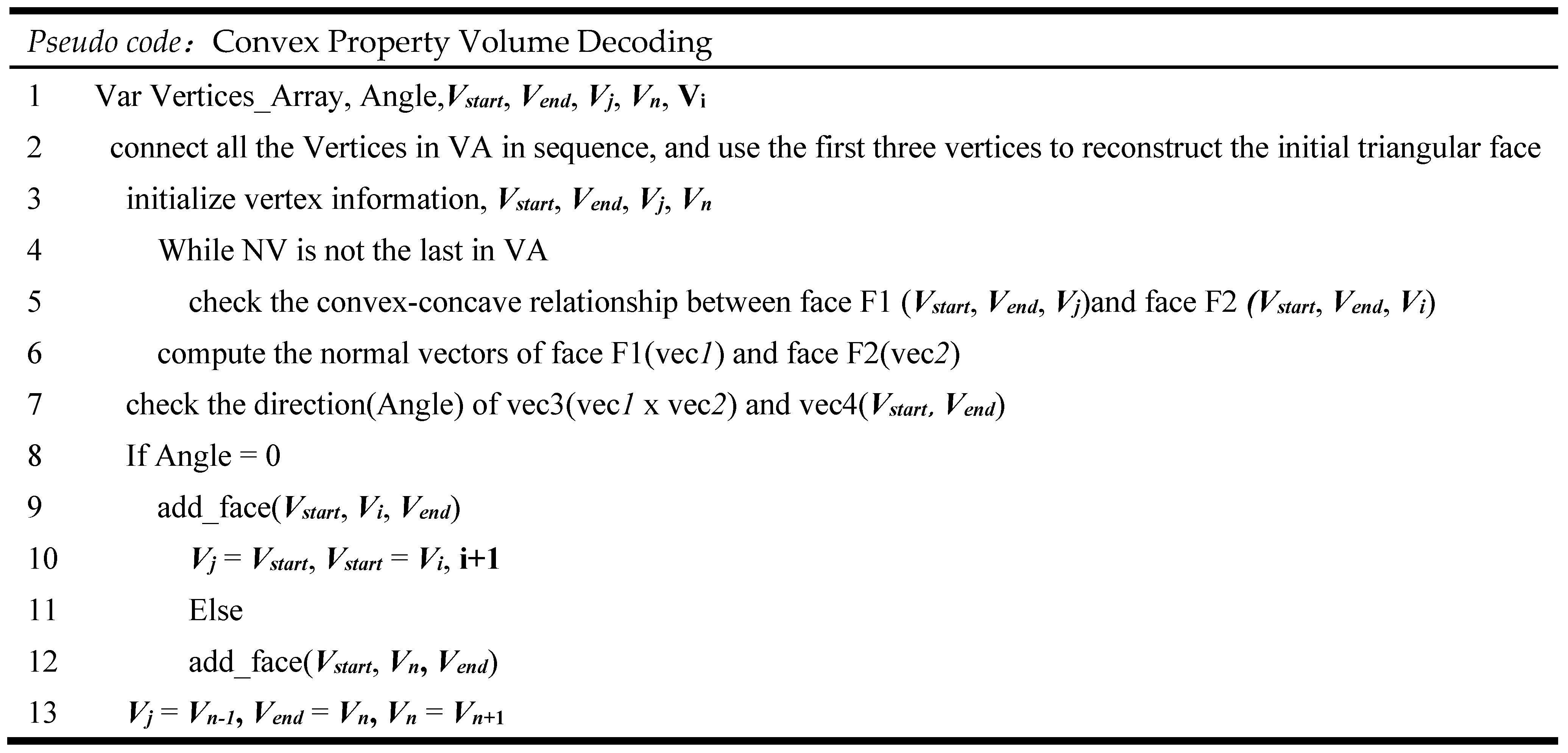
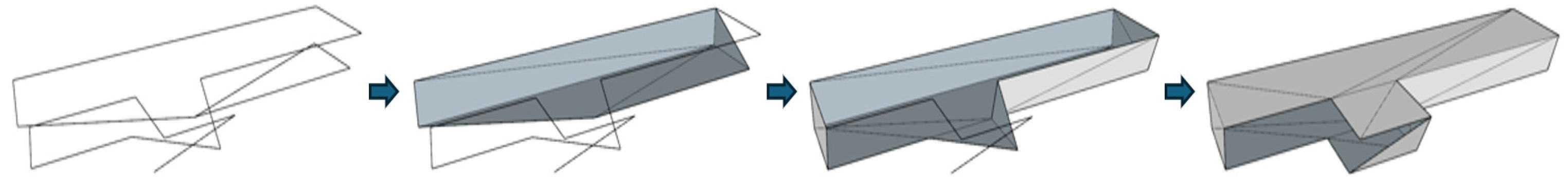
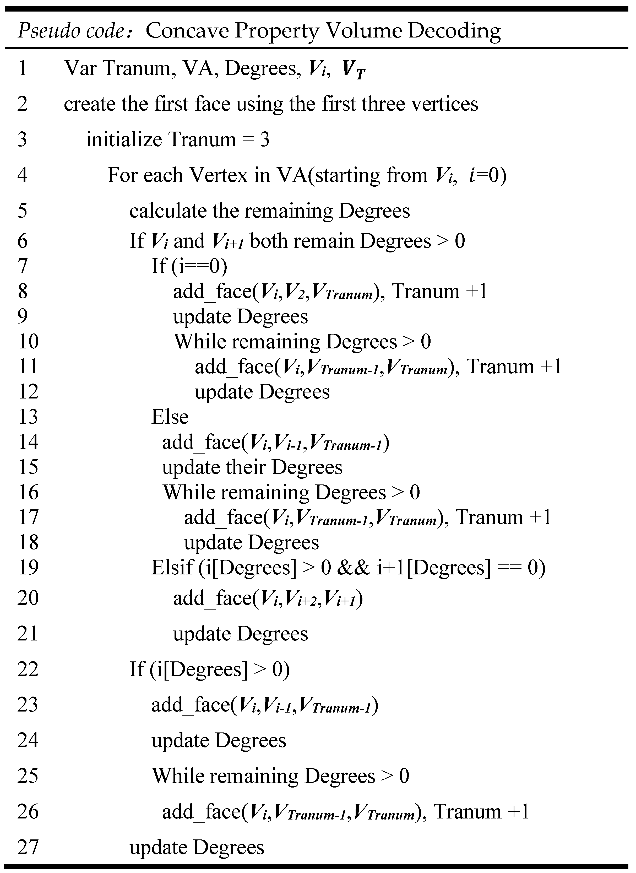
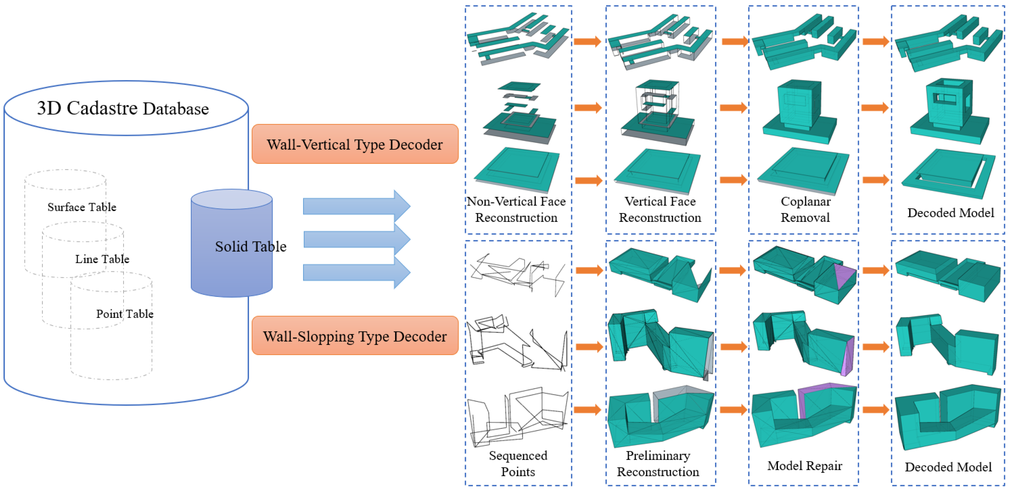
According to the Wall-Sloping Property Volume characteristics, it is further subdivided into two categories: convex property volume models and concave property volume models. The Angle between all adjacent faces of the convex model is less than 180 degrees. In the encoding process, the triangles contained in each face are traversed by the spiral expansion of edges, and the corresponding vertex information is recorded in turn, and the vertex information is stored as a vertex sequence. For this type of 3D property volume, its surface must be triangulated to construct a mesh structure, enabling the conversion of smooth model encoding into triangular surface encoding. The triangulation process is illustrated in Figure 6. Beginning at an arbitrary point, the diagonals of the shape are connected sequentially until all surface shapes are divided into triangles.
After completing the triangulation, the entire point set of the property volume is systematically traversed by leveraging the adjacency relationships. Specifically, any triangular face in the triangular mesh can serve as a seed face. One of its edges is randomly chosen as the starting edge for traversal. The traversal process proceeds as follows in Figure 7: the vertex adjacent to the endpoint of the starting edge in the right-hand adjacent triangular face relative to the current traversal edge is identified. If this vertex has not yet been traversed, it is marked as visited and becomes the starting point for the next traversal edge. If the edge has already been traversed, the endpoint of the current traversal edge is updated to the next vertex in sequence while keeping the start point unchanged. Through cyclic traversal, a complete one-dimensional vertex sequence is obtained.
The coding process of convex property volume can be referred to Figure 8. We introduce three variables for the model: NTA to store the vertices that have not yet been traversed, TA to store the vertices that have already been traversed, and VA to store the encoded vertex sequence. Additionally, Vstart denotes the starting point of the currently traversed edge, Vend denotes the endpoint of the currently traversed edge, and Vright denotes a vertex on the triangular face to the right of the currently traversed edge.
In Figure 9, for concave model structures that may contain angles greater than 180 degrees, the encoding process must not only capture the geometric information of vertices and faces but also incorporate relational data describing the adjacency of vertices. This adjacency information plays a critical role in accurately reconstructing the geometry of the concave model during the reduction process, thereby preventing geometric errors or face overlaps.
Figure 10 illustrates the triangulation process of the face in the concave model. For the triangulated model, a triangular face is selected as the seed, and its vertices are identified. Each vertex contains adjacency information to other triangular faces. Starting from any vertex, all adjacent faces are traversed counterclockwise, and the number of adjacencies (denoted as the degree) is recorded. Simultaneously, unvisited vertices are encoded in counterclockwise order. If a previously visited vertex is encountered during traversal, the process for that vertex is terminated. The next unvisited vertex in the sequence is then selected as the new traversal point, and its adjacent faces are cyclically traversed until all triangular faces and vertices of the model have been traversed. This results in a complete one-dimensional vertex sequence.
The dimensionality reduction coding process of the concave volume model can be referred to in Figure 11. We define the variable NTA to store the vertices that have not yet been traversed in the model, TA to store the vertices that have already been traversed, and VA to store the encoded vertex sequence. Additionally, Vstart denotes the starting point of the currently traversed edge, Vend denotes the endpoint of the currently traversed edge, Vright denotes a vertex on the right triangular face of the currently traversed edge, and Vth denotes a vertex on the left triangular face of the currently traversed edge.

3.4. Decoder

Decoding is the process of reconstructing the vertex, edge and face structure of the 3D model by parsing the encoded point set sequence.

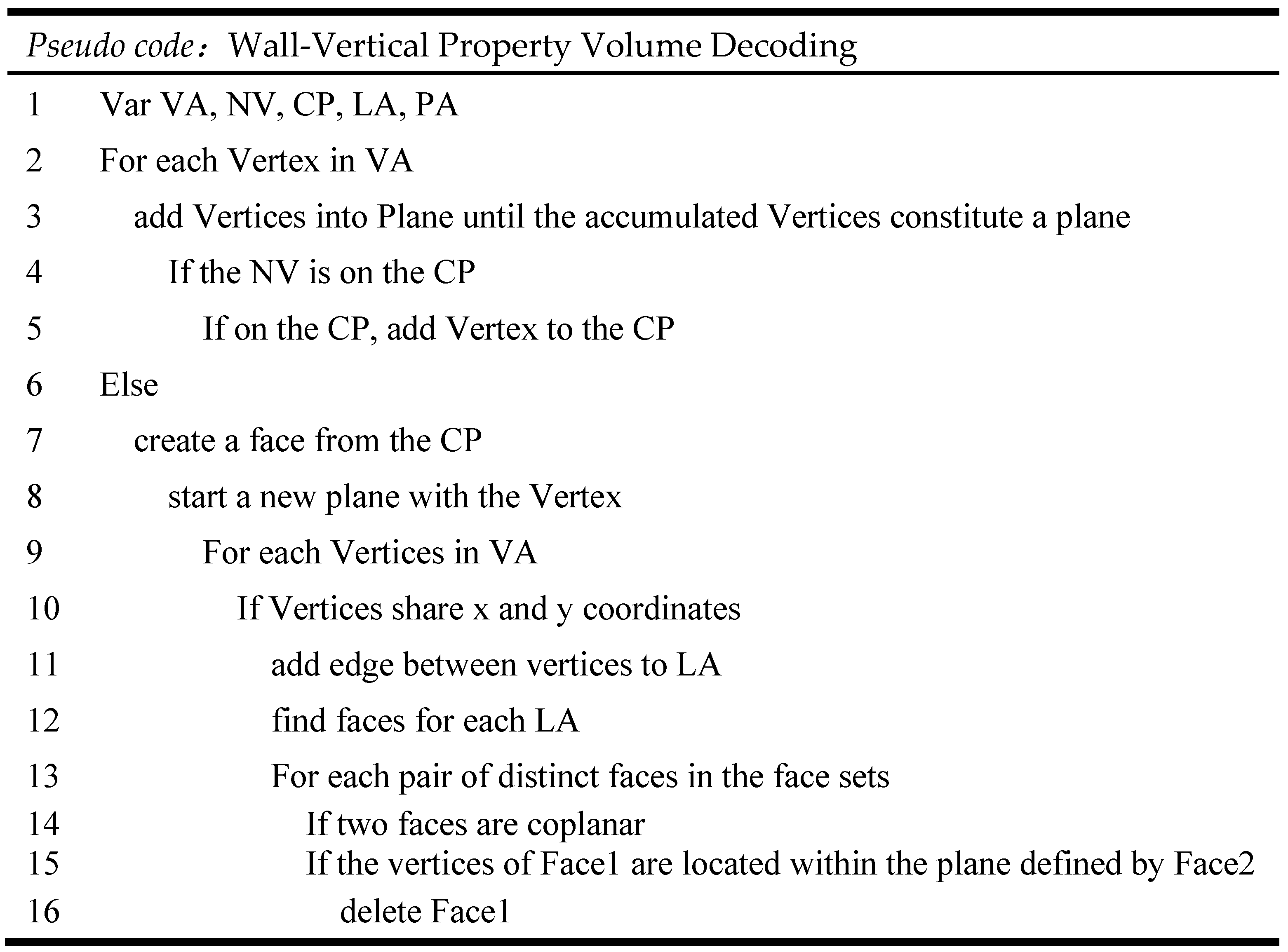
3.4.1. Decoding Process for the Vertical Type

The Vertical type typically features a symmetrical structure in the vertical direction. Data are read from the database based on prefabricated sequence, and each parallel surface is reconstructed sequentially according to varying height values, as illustrated in Figure 12.
Decoder process: Initially, three consecutive vertices from the sequence of points are read and output in order. Subsequently, we verify whether these three vertices are collinear. If they are, additional vertices are evaluated until a set of vertices that are not coplanar is obtained, which is then used to construct the initial starting face. Once a plane is established, if a new vertex exhibits a coplanar relationship with the current plane, it is incorporated into the current plane until a vertex is encountered that does not belong to the current plane. The vertices of the current plane are then sequentially connected to reconstruct the non-coplanar plane. Finally, the spatial relationships between all planes are assessed. In cases where intersecting relationships exist between planes, the intersecting planes are removed.
The decoding process of the Vertical type can be referred to in Figure 13. We define the variable VA to store the sequence of vertices encoded by the encoder. Additionally, the variable NV indicates the next vertex to be traversed, CP represents the plane associated with the currently traversed vertex, LA is defined as the set of vertical edges within the model, and FA denotes the set of faces in the model.

3.4.2. Decoding Process for the Slope Model

Due to the concave-convex structure of sloping-type models, the decoding process is divided into two categories accordingly.
For convex types, the decoding operations for convex property volume models are primarily based on spiral traversal (Figure 14). Initially, all vertices are sequentially connected to form the “skeleton” of the model. Subsequently, according to the spiral traversal order, all adjacent triangular faces of the currently traversed vertex are reconstructed. In a 2-manifold, each edge is shared by exactly two triangular facets. Based on this principle, for the currently traversed edge, a third vertex must be checked to construct the triangular face. To ensure that the triangular facet is closed, there are two potential cases for the third vertex: either the next vertex in the order table that has not yet been traversed or the vertex immediately following the currently traversed vertex. The selection of the vertex is checked by analyzing the normal relationship between the adjacent faces of the convex model. The concavity or convexity of the triangular facet formed by the traversal edge and two vertices, as well as the triangular facet constructed in the previous step, is evaluated. By analyzing the relationship between the normal vectors, it is checked whether the angle between the new triangular facet and the old triangular facet is a convex angle. This confirms that the current vertex serves as the third vertex of the next triangular face. If the triangular faces are coplanar, the vertex immediately following the currently traversed vertex is used to reconstruct the triangular faces according to the triangulation algorithm principle. Once all the adjacent faces of the currently traversed vertex are constructed, the traversal proceeds to the next vertex in order, and the iteration is repeated until all the triangular faces that can be preliminarily recovered are reconstructed.
The decoding process of convex volume model can be referred to Figure 15. We define the variable VA to store the vertex sequence encoded by the encoder, and the variable Angle to check whether the face to be generated should be a closed face or a new triangular face. Vstart represents the starting point of the traversed edge, Vend represents the end point of the traversed edge, Vj represents a vertex in the triangle face currently processed, Vn represents the vertex to be closed, and Vi represents the third vertex of the next triangle face.
For concave types (Figure 16), in cases where convex angles are possible, the number of adjacent points is augmented by the “degree” value recorded during encoding to ensure precise reconstruction of the model. Unlike the convex type, during “skeleton” construction, the degree is calculated concurrently and progressively decreased until it reaches zero as the triangular faces are filled.
The corresponding decoding algorithm is shown in Figure 17. We define the variable Tranum to represent a vertex index in the currently processed triangular face, the variable VA to store the encoded vertex sequence generated by the encoder, the variable Degrees to denote the degree of a vertex, and the variable V i to indicate the current traversal vertex. Notably, V T specifically refers to a vertex within the triangular face being processed.

3.5. Repair Process

For the 3D property volume of slope type, the model may contain holes. This issue arises because, during the decoding process, the surface filling step involves a decoding order and triangular face orientation that differ from those used during encoding. Consequently, this mismatch leads to unsuccessful surface filling, necessitating further repair. The hole repair is conducted using the triangle filling method. As shown in Figure 18, the repair process begins with the extraction of the hole boundary, which typically comprises one or more closed contours formed by unclosed edges. Subsequently, the boundary is traversed to identify the vertices and edges of the hole. Triangular facets are then incrementally created by selecting adjacent vertices, gradually filling the hole. This procedure is iteratively repeated until the hole is entirely filled.
De-Triangulation: As a further optimization step for the model, the core concept relies on the coplanar relationship among faces. During processing, all adjacent faces that are coplanar with any given triangle are identified. Based on the coplanar relationships among these faces, the outer boundary lines are retained while the inner connecting lines are eliminated. A schematic of the execution process is shown in Figure 19. The combination of coplanar triangles (1, 3), (2, 4, 7), (5, 6), after eliminating the internal lines, forms three new independent shapes.
Following the De-Triangulation process, coplanar redundant triangles are consolidated into a single polygon, which serves to represent the boundary of the 3D property volume.

4. Case Study

4.1. Data and the Experimental Environment

As a technical validation, to avoid potential legal disputes, we conducted an experiment using simulated three-dimensional property rights of building types. Specifically, we extracted six complex real-world building spatial structures from Shenzhen University (located in Guangdong Province, China; the geographical center of the case area is at WGS84 coordinates: longitude 113.936° E and latitude 22.533° N) as the simulated 3D property volume models. Their locations are illustrated in Figure 20 using the Web Mercator projection (EPSG:3857). Among these, Model 1, Model 2, and Model 3 represent Vertical-Type structures, while Model 4, Model 5, and Model 6 incorporate several inclined planes, denoted as Slopping-Type 3D property volume. Our experimental setup includes SketchUp 2024 scripting, leveraging SketchUp’s built-in encapsulation for point, line, surface, and body topological relationships, implemented via Ruby-based secondary development. The experiments were executed on a workstation equipped with a 2.90 GHz Intel Core CPU, 64 GB RAM, and an NVIDIA GeForce GTX 3070 GPU.

4.2. Encoding and Decoding Experiments of 3DPV-CC

The models of the six cases have been stored in the 3D cadastre database following the “point-line-surface” structure. Figure 21a illustrates the data table configurations for case 2 and case 4. Despite the original point sets of case 2 and case 4 containing only 64 points and 49 points, respectively, both cases still require additional storage of line and surface tables in the database: case 2 (96 lines, 37 surfaces) and case 4 (79 lines, 32 surfaces). To encode the 3D property volumes model, we applied the 3DPV-CC method and created a unique solid table to store the reordered point set, point coordinates, and corresponding degree information. The reorganized data structure is presented in Figure 21b. Apart from case 2 and case 4, the structures of the other cases are similar.
Figure 22 illustrate the decoding and reconstruction processes of the Wall-vertical type 3D property volume and the Wall-slopping type 3D property volume. The 3DPV-CC scheme can successfully restore all models from the database into 3D models, meeting the requirements for visualization and 3D cadastral mapping. In the process of model decoding, the variation in the selection of initial seed points can lead to discrepancies in the positioning of triangular surfaces for the Wall-slopped type model during surface restoration. Nevertheless, these discrepancies do not influence the final visualization outcomes.

4.3. The Effect Analysis

The encoding and decoding process of 3D Property Volume is fundamentally a data compression and reconstruction process. To evaluate the performance of the 3DPV-CC method in handling 3D Property Volume models, we employ the Compression Rate (as defined in Equation (1)) and the Recovery Rate (as defined in Equation (2)).
The Compression Rate is defined as the ratio of the encoded data size to the original model data size, with its complement calculated as the difference from 1. A higher compression rate indicates a greater reduction in redundant data, which enhances the efficiency of data storage in databases.
C ompression   Rate   = ( 1 C o m p r e s s e d   S i z e O r i g i n a l   S i z e ) × 100 % ,
The restore rate reflects the decoding method’s inherent ability to automatically restore data from the database into a visual model. RFs denotes the number of surfaces successfully recovered during the decoding process, while OFs represents the total number of surfaces contained in the original 3D Property Volume model.
R e c o v e r y   R a t e = R F s O F s × 100 %
Table 1 presents the performance of the original 3D property volume model, and the model processed by the 3DPV-CC method. For the wall-vertical type, a larger model size generally leads to a better compression effect. For instance, in case 1, the size is reduced from 20.3 KB to 12.5 KB, achieving a compression ratio of 38.42%. In case 3, the size is compressed from 12.6 KB to 9.48 KB, with a compression ratio of 24.76%. The average compression ratio for this type is 31.71%. For the wall-slopped type, the compression ratios for the three cases are 27.86%, 27.67%, and 23.66%, respectively, resulting in an average compression ratio of 26.39%, which is lower than that of the wall-vertical type. The average compression ratio for all cases is 29.05%. Additionally, the 3DPV-CC method can fully restore all surfaces of the wall-vertical type, while the restoration performance for the wall-slopped type remains consistently above 93%.
We also try to compare 3DPV-CC with some general data compression algorithms (ZIP/7Z/RAR), and the results of the comparison are presented in Table 2. In the ZIP method, the model’s compression rates are 8.37%, 9.52%, 9.52%, 9.29%, 8.81%, and 9.16%, respectively. In the 7Z method, the compression rates are 9.36%, 9.52%, 10.32%, 10.0%, 8.81%, and 9.92%, respectively. In the RAR compression method, the compression rates are 8.87%, 9.52%, 10.32%, 10.0%, 8.81%, and 9.92%, respectively. It is evident that general compression algorithms exhibit lower compression efficiency compared to 3DPV-CC; however, they demonstrate a more stable and consistent compression ratio.

4.4. Discussion

Our experiments demonstrate that the 3DPV-CC algorithm can effectively encode and decode the wall-vertical and wall-slopped 3D property volumes, showcasing its unique advantages. These advantages are primarily reflected in three aspects: (1) When storing the coded data in the database, only point tables need to be recorded, rather than line and surface tables, as detailed in Section 4.2. By reducing the data tables, the structural information (in this paper, the topology structure) of the data is concealed in a specific sequence of the point string. (2) The overall data compression capacity of the 3DPV-CC algorithm surpasses that of conventional data compression algorithms, as is evident from the comparative analysis in Section 4.3. For instance, the compression ratio of case 1 is approximately 30% higher than that of algorithms such as ZIP/7Z/RAR, and the compression ratio of case 6 is also around 13% higher than that of general algorithms. (3) Based on the types of 3D property volume currently summarized by scholars (Section 2), the 3DPV-CC algorithm enables the complete reconstruction of the vertical type of 3D property volume and the partial reconstruction of the inclined wall type. However, it is clear to us that with the wider implementation of field investigations for 3D property volume, more morphological types may emerge [30].
However, it is important to note that the 3DPV-CC method has certain limitations. For instance, its compression stability is relatively low, with varying compression ratios across different 3D property volume models. The low stability under compression is attributed to the inherent geometric complexity (such as the number of points, lines, and surfaces) and topological complexity (the relative positions and connections between geometric elements) of 3D property volumes. This is especially true for wall-sloped types, which necessitate additional topological information (the degree mentioned in Section 3) to maintain structural accuracy. As a result, compared to the more regular wall-vertical volumes, they exhibit less consistent compression ratios. Additionally, the recovery ability for wall-slopped types requires further improvement due to the potential risk of surface data loss, which cannot be fully assessed using only three test models.

5. Conclusions

Cadastral management has transitioned from the traditional paper-based era to a phase of spatial database management supported by 3D GIS. The 3D property volumes serve as a critical data carrier for 3D cadastral systems, which are essential for modern 3D land administration. Current research on 3D cadastres frequently focuses on isolated special cases. As the number of 3D property volume cases grows, scholars have begun to emphasize the classification of 3D property volumes; however, this area remains in its infancy. From the perspective of urban land management, storing large amounts of 3D property volume data in databases is an inevitable requirement. Many challenges arise in managing and storing massive amounts of 3D property volume data within complex spatial frameworks, such as low-altitude space right modeling [31]. For instance, in Shenzhen, as of January 2024, the total number of housing units reached 12.68 million. If all these units were converted into comprehensive 3D property volume datasets, their size might exceed the capacity limits of conventional databases.
Therefore, this paper proposes a 3DPV-CC method, enabling the 3D property volume model to be stored in the database at a low cost and reconstructed into a model with 3D topology for visualization when necessary. The experimental results demonstrate that the 3DPV-CC method offers certain advantages and potential in improving the efficiency of 3D cadastral management and simplifying property volume expression, providing a new approach for representing 3D topology models in traditional 3D GIS. Although this method can effectively compress 3D property volume data with specific regular structures in the database and support the production and visualization of 3D parcel maps, there is still room for improvement in the encoding strategy. For instance, a common algorithm could be developed for two sloping-type 3D property volumes, rather than using separate algorithms for each type. Furthermore, future work will focus on advancing the following areas: (1) for complex 3D cadastre scenes, research on technologies for handling the simultaneous loading of a large number of 3D property volumes based on visibility and R-tree spatial index methods [32]; (2) the transfer of some proprietary or cross-domain technologies may help us further process extremely complex three-dimensional property volume data. For instance, the 3D-SPIHT algorithm for CT scan data achieves efficient compression of volumetric data through a combination of slicing and treeing [33,34]; (3) since the current evaluation focuses only on data size, it represents a compromise when compared with general compression algorithms. Therefore, proprietary evaluation metrics for geometry and topology should be refined to enable more accurate quantitative assessments; (4) furthermore, with an eye towards the potential future realization of city-level 3D property volume awareness, deep learning techniques will be contemplated in the future. This is to effectively leverage computing power for problem-solving purposes.

Author Contributions

Conceptualization, Zhigang Zhao and Chengpeng Li; methodology, Chengpeng Li; software, validation, formal analysis, Jiahao Qiu; resources, Han Guo and Wei Zhu; writing—original draft preparation, Chengpeng Li; project administration, Zhigang Zhao; funding acquisition, Chengpeng Li. All authors have read and agreed to the published version of the manuscript.

Funding

This research was funded by the Open Research Fund Program of Key Laboratory of Digital Mapping and Land Information Application, Ministry of Natural Resources (ZRZYBWD202403) and the National Natural Science Foundation of China (NSFC) (No. 42171265 and No. 62394335).

Data Availability Statement

All data are available at the open-source data warehouse (GitHub) https://github.com/fxkulou/3DPV-CC (accessed on 2 July 2025).

Conflicts of Interest

The authors declare no conflict of interest.

References

  1. Kalogianni, E.; van Oosterom, P.; Dimopoulou, E.; Lemmen, C. 3D Land Administration: A Review and a Future Vision in the Context of the Spatial Development Lifecycle. ISPRS Int. J. Geo-Inf. 2020, 9, 107. [Google Scholar] [CrossRef]
  2. Li, C.; Zhao, Z.; Chen, Y.; Zhu, W.; Qiu, J.; Jiang, S.; Guo, R. Modeling the Urban Low-Altitude Traffic Space Based on the Land Administration Domain Model—Case Studies in Shenzhen, China. Land 2024, 13, 2062. [Google Scholar] [CrossRef]
  3. Kalogianni, E.; Dimopoulou, E.; Thompson, R.; Lemmen, C.; Ying, S.; van Oosterom, P. Development of 3D spatial profiles to support the full lifecycle of 3D objects. Land Use Policy 2020, 98, 104–177. [Google Scholar] [CrossRef]
  4. Zhang, J.-Y.; Yin, P.-C.; Li, G.; Gu, H.-H.; Zhao, H.; Fu, J.-C. 3D Cadastral Data Model Based on Conformal Geometry Algebra. ISPRS Int. J. Geo-Inf. 2016, 5, 20. [Google Scholar] [CrossRef]
  5. Ying, S.; Chen, N.; Li, W.; Li, C.; Guo, R. Distortion visualization techniques for 3D coherent sets: A case study of 3D building property units. Comput. Environ. Urban Syst. 2019, 78, 101382. [Google Scholar] [CrossRef]
  6. Salleh, S.; Ujang, U.; Azri, S. Topological Relationships in R3 for 3d Cadastre. Int. Arch. Photogramm. Remote Sens. Spat. Inf. Sci. 2022, 48, 165–170. [Google Scholar] [CrossRef]
  7. Emamgholian, S.; Taleai, M.; Shojaei, D. Exploring the applications of 3D proximity analysis in a 3D digital cadastre. Geo-Spat. Inf. Sci. 2021, 24, 201–214. [Google Scholar] [CrossRef]
  8. Jaljolie, R.; Riekkinen, K.; Dalyot, S. A topological-based approach for determining spatial relationships of complex volumetric parcels in land administration systems. Land Use Policy 2021, 109, 105637. [Google Scholar] [CrossRef]
  9. Sun, J.; Mi, S.; Olsson, P.-O.; Paulsson, J.; Harrie, L. Utilizing BIM and GIS for Representation and Visualization of 3D Cadastre. ISPRS Int. J. Geo-Inf. 2019, 8, 503. [Google Scholar] [CrossRef]
  10. Ying, S.; Guo, R.; Li, L.; Van Oosterom, P.; Stoter, J. Construction of 3D volumetric objects for a 3D cadastral system. Trans. GIS 2015, 19, 758–779. [Google Scholar] [CrossRef]
  11. Guo, R.; Li, L.; Ying, S.; Luo, P.; He, B.; Jiang, R. Developing a 3D cadastre for the administration of urban land use: A case study of Shenzhen, China. Comput. Environ. Urban Syst. 2013, 40, 46–55. [Google Scholar] [CrossRef]
  12. Asghari, A.; Kalantari, M.; Rajabifard, A. Advances in techniques to formulate the watertight concept for cadastre. Trans. GIS 2021, 25, 213–237. [Google Scholar] [CrossRef]
  13. Knoth, L.; Atazadeh, B.; Rajabifard, A. Developing a new framework based on solid models for 3D cadastres. Land Use Policy 2020, 92, 104480. [Google Scholar] [CrossRef]
  14. Asghari, A.; Kalantari, M.; Rajabifard, A. A structured framework for 3D cadastral data validation− a case study for Victoria, Australia. Land Use Policy 2020, 98, 104359. [Google Scholar] [CrossRef]
  15. Thompson, R.; van Oosterom, P.; Soon, K.H. A Conceptual Model supporting a range of 3D parcel representations through all stages: Data Capture, Transfer and Storage. In FIG Working Week; International Federation of Surveyors: Copenhagen, Denmark, 2016; Volume 2. [Google Scholar]
  16. Kalogianni, E.; Dimopoulou, E.; Greece, R. Investigating 3D spatial units’ types as basis for refined 3d spatial profiles in the context of LADM revision. In Proceedings of the 6th International FIG Workshop on 3D Cadastres, Delft, The Netherlands, 2 October 2018. [Google Scholar]
  17. Ying, S.; Li, C.; Chen, N.; Jia, Y.; Guo, R.; Li, L. Object Analysis and 3D Spatial Modelling for Uniform Natural Resources in China. Land 2021, 10, 1154. [Google Scholar] [CrossRef]
  18. Deering, M. Geometry compression. In Proceedings of the 22nd Annual Conference on Computer Graphics and Interactive Techniques, Los Angeles, CA, USA, 6–11 August 1995; pp. 13–20. [Google Scholar]
  19. Bajaj, C.L.; Pascucci, V.; Zhuang, G. Single resolution compression of arbitrary triangular meshes with properties. Comput. Geom. 1999, 14, 167–186. [Google Scholar] [CrossRef]
  20. Janečka, K.; Váša, L. Compression of 3D geographical objects at various level of detail. In The Rise of Big Spatial Data; Springer International Publishing: Cham, Switzerland, 2016; pp. 359–372. [Google Scholar]
  21. Gurung, T.; Luffel, M.; Lindstrom, P.; Rossignac, J. Zipper: A compact connectivity data structure for triangle meshes. Comput. Aided Des. 2013, 45, 262–269. [Google Scholar] [CrossRef]
  22. Siddeq, M.M.; Rodrigues, M.A. Novel 3D compression methods for geometry. connectivity and texture. 3D Res. 2016, 7, 1–18. [Google Scholar] [CrossRef]
  23. Nguyen, V.P.; Ung, E.M.; Krishna, A.; Tham, S. Lossless compression of topology of 3D triangulated irregular networks. In Proceedings of the 10th International Conference on Information, Communications and Signal Processing (ICICS), Singapore, 2–4 December 2015; IEEE: Piscataway, NJ, USA, 2015; pp. 1–5. [Google Scholar]
  24. Wei, W.; Liu, Y.; Duan, X.; Guo, C. Representation method of 3D model mesh chain code. J. Comput. Aided Des. Comput. Graph. 2017, 29, 537–548. [Google Scholar]
  25. Li, M.; Nan, L. Feature-preserving 3D mesh simplification for urban buildings. ISPRS J. Photogramm. Remote Sens. 2021, 173, 135–150. [Google Scholar] [CrossRef]
  26. Lin, D.; Zhao, C.; Tian, Q.; Xu, Y.; Wang, R.; Qu, Z. GMM-ICQ: A GMM vertex-optimization-based implicitly-connected quadrilateral format for 3D mesh storage. Comput. Graph. 2024, 118, 34–47. [Google Scholar] [CrossRef]
  27. Zhao, X.; Zeng, X.; Gao, L.; Xu, Y.; Wang, Y. DMGC: Deep Triangle Mesh Geometry Compression via Connectivity Prediction. In Proceedings of the 33rd Workshop on Network and Operating System Support for Digital Audio and Video, Vancouver, BC, Canada, 7–10 June 2023; pp. 15–21. [Google Scholar]
  28. Wang, Z.; Zhou, S.; Park, J.J.; Paschalidou, D.; You, S.; Wetzstein, G.; Guibas, L.; Kadambi, A. Alto: Alternating latent topologies for implicit 3d reconstruction. In Proceedings of the IEEE/CVF Conference on Computer Vision and Pattern Recognition, Vancouver, BC, Canada, 18–22 June 2023; pp. 259–270. [Google Scholar]
  29. Balreira, D.G.; da Silveira, T.L.T. Triangular matrix-based lossless compression algorithm for 3D mesh connectivity. Vis. Comput. 2024, 40, 3961–3970. [Google Scholar] [CrossRef]
  30. Li, L.; Guo, R.; Ying, S.; Zhu, H.; Wu, J.; Liu, C. 3D Modeling of the Cadastre and the Spatial Representation of Property. In Urban Informatics; Springer: Berlin/Heidelberg, Germany, 2021; pp. 589–607. [Google Scholar]
  31. Li, C.; Kuai, X.; He, B.; Zhao, Z.; Lin, H.; Zhu, W.; Liu, Y.; Guo, R. Visibility-Based R-Tree Spatial Index for Consistent Visualization in Indoor and Outdoor Scenes. ISPRS Int. J. Geo-Inf. 2023, 12, 498. [Google Scholar] [CrossRef]
  32. Li, C.; Guo, R.; Zhao, Z.; He, B.; Kuai, X.; Wang, W.; Chen, X. Conceptual Modeling Method for Urban Low-Altitude Passage Easement. J. Geo-Inf. Sci. 2024, 26, 1811–1826. [Google Scholar]
  33. Cho, S.; Kim, D.; Pearlman, W.A. Lossless Compression of Volumetric Medical Images with Improved Three-Dimensional SPIHT Algorithm. J. Digit. Imaging 2004, 17, 57–63. [Google Scholar] [CrossRef]
  34. Xiong, Z.; Wu, X.; Cheng, S.; Hua, J. Lossy-to-lossless compression of medical volumetric data using three-dimensional integer wavelet transforms. IEEE Trans. Med. Imaging 2003, 22, 459–470. [Google Scholar] [CrossRef]
Figure 1. The one–to–one mapping between the 3D property volume and the database table.
Ijgi 14 00263 g001
Figure 2. The seven types of 3D Property Volume (Concluded from references [15,16]).
Ijgi 14 00263 g002
Figure 3. The 3DPV-CC.
Ijgi 14 00263 g003
Figure 4. The process of encoding the Wall-Vertical Property Volume.
Ijgi 14 00263 g004
Figure 5. The Pseudo code of “Wall-Vertical Property Volume encoding”.
Ijgi 14 00263 g005
Figure 6. Triangulation of a face in the convex model.
Ijgi 14 00263 g006
Figure 7. The process of encoding the Convex Property Volume.
Ijgi 14 00263 g007
Figure 8. The Pseudo code of “Convex Property Volume Encoding”.
Ijgi 14 00263 g008
Figure 9. Triangulation of a face in the concave model.
Ijgi 14 00263 g009
Figure 10. The triangulation of a face in the concave model.
Ijgi 14 00263 g010
Figure 11. The Pseudo code of “Concave Property Volume Encoding”.
Ijgi 14 00263 g011
Figure 12. The process of decoding the Wall-Vertical Property Volume.
Ijgi 14 00263 g012
Figure 13. The Pseudo code of “Wall-Vertical Property Volume decoding”.
Ijgi 14 00263 g013
Figure 14. The process of decoding the Convex Property Volume.
Ijgi 14 00263 g014
Figure 15. The Pseudo code of “Convex Property Volume decoding”.
Ijgi 14 00263 g015
Figure 16. The process of decoding the Concave Property Volume.
Ijgi 14 00263 g016
Figure 17. The Pseudo code of “Concave Property Volume decoding”.
Ijgi 14 00263 g017
Figure 18. The process of triangle filling.
Ijgi 14 00263 g018
Figure 19. The process of De-Triangulation.
Ijgi 14 00263 g019
Figure 20. The physical building position in Shenzhen University (in Guangdong Province, China).
Ijgi 14 00263 g020
Figure 21. Encoding the 3D property volumes in 3D cadastre database: (a) Case2; (b) Case4.
Ijgi 14 00263 g021
Figure 22. Decoding the 3D Property Volumes from 3D cadastre database.
Ijgi 14 00263 g022
Table 1. Encoding and decoding performance of 3DPV-CC.
No.The Original State3DPV-CC
PointLineSurfaceSize (KB)Compressed Size (KB)Compression RateRecovery Rate
Case 11231907820.312.538.42%100%
Case 264963714.710.031.97%100%
Case 332482112.69.4824.76%100%
Case 44979321410.127.86%93.62%
Case 5691104315.911.527.67%96.27%
Case 638602413.110.023.66%93.15%
Table 2. A comparison of 3DPV-CC with general compression methods.
No.Original Size
(KB)
3DPV-CCZIP7ZRAR
SizeRatioSizeRatioSizeRatioSizeRatio
Case 120.312.538.42%18.68.37%18.49.36%18.58.87%
Case 214.71031.97%13.39.52%13.39.52%13.39.52%
Case 312.69.4824.76%11.49.52%11.310.32%11.310.32%
Case 41410.127.86%12.79.29%12.610.0%12.610.0%
Case 515.911.527.67%14.58.81%14.58.81%14.58.81%
Case 613.11023.66%11.99.16%11.89.92%11.89.92%
Disclaimer/Publisher’s Note: The statements, opinions and data contained in all publications are solely those of the individual author(s) and contributor(s) and not of MDPI and/or the editor(s). MDPI and/or the editor(s) disclaim responsibility for any injury to people or property resulting from any ideas, methods, instructions or products referred to in the content.

