Geometry and Topology Correction of 3D Building Models with Fragmented and Disconnected Components

Abstract

This paper presents a methodology for correcting geometric and topological errors, specifically addressing fragmented and disconnected components in buildings (FDCB) in 3D models intended for urban digital twin (UDT). The proposed two-stage approach combines geometric refinement via duplicate vertex removal with topological refinement using a novel spatial partitioning-based Depth-First Search (DFS) algorithm for connected mesh clustering. This spatial partitioning-based DFS significantly improves upon traditional graph traversal methods like standard DFS, breadth-first search (BFS), and Union-Find for connectivity analysis. Experimental results demonstrate that the spatial DFS algorithm significantly improves computational speed, achieving processing times approximately seven times faster than standard DFS and 17 times faster than BFS. In addition, the proposed approach achieves a data size ratio of approximately 20% in the simplified mesh, compared to the 50–60% ratios typically observed with established techniques like Quadric Decimation and Vertex Clustering. This research enhances the quality and usability of 3D building models with FDCB issues for UDT applications.

1. Introduction

Urban digital twin (UDT) is a core technology that can be used in various fields such as urban planning, facility management, and disaster prediction by identically implementing an actual city in a virtual space [1]. The accuracy and utility of a UDT are contingent upon the precise construction of 3D models representing urban components such as buildings, roads, and terrain. In particular, buildings are one of the crucial elements constituting a city, and in UDT, 3D building models are used for various purposes, such as simulation, visualization, and analysis. Recently, research to rapidly construct 3D building models of large-scale cities using multiple technologies such as airborne LiDAR, drones, and photogrammetry has been active [2,3,4].

Platforms such as Google Earth [5] and VWorld [6] provide 3D models of entire cities across the globe or in specific countries. Google Earth utilizes various sources, including satellite imagery, aerial photography, and LiDAR data, to construct 3D building models of major cities worldwide. VWorld is a platform operated by the Ministry of Land, Infrastructure, and Transport of South Korea, providing 3D spatial information of the entire nation based on aerial photographs and LiDAR data. The 3D building models offered by these platforms number hundreds of thousands to millions, boasting a vast scale encompassing entire cities. UDT construction is based on such large-scale 3D model data and includes various objects such as roads, bridges, tunnels, terrain, and vegetation, in addition to buildings [7].

3D building model construction is classified into automatic, semi-automatic, and manual methods. The automatic method utilizes airborne LiDAR data or satellite imagery to automatically generate building models, enabling rapid construction of large-scale area models, but it lacks accuracy and detail [8]. The semi-automatic method involves the user creating an initial model or setting some parameters to assist model generation, which results in higher accuracy than the automatic method but requires user intervention [9]. The manual method involves the user directly creating the model using 3D modeling software, allowing for the creation of the most accurate and detailed model, but it requires a lot of time and effort [10].

For city-scale UDT construction, a process of integrating 3D models acquired from various sources is required. However, these models vary in quality depending on the data acquisition method, modeling technique, and worker skill level, and some models cause difficulties in UDT application. In particular, when multiple unskilled workers participate in constructing many 3D building models, there is a high possibility that abnormal or inefficient building models will be generated. For example, when applying a semi-automatic modeling technique based on two or more images taken from an aircraft, problems may occur when the worker creates polygons by matching identical points and converting them into a 3D model. In this case, the generated building model is not a single solid model but a form in which multiple polygons in the form of faces or triangles are gathered without connectivity [11]. This paper defines this as the problem of fragmented and disconnected components in buildings (FDCB). Building models with the FDCB problem can have various errors that degrade quality. To solve these problems, 3D model inspection methods are used [12]. However, existing 3D model inspection methods mainly target automatically generated models or sophisticated models created in CAD systems and thus have limitations in effectively handling special error types (duplicate points, disconnection, non-watertight structures, etc.) inherent in large-scale city models created manually or semi-automatically by unskilled workers.

Algorithms have been developed to identify and correct geometric errors in 3D models, such as duplicate vertices, overlapping faces, and abnormal normal vectors; these are commonly integrated into commercial 3D modeling software [13,14,15]. Research has also addressed topological errors, with algorithms to assess face orientation, boundary connectivity, and self-intersections, thereby ensuring topological consistency [16]. However, these methods do not fully address disconnection problems. This issue is particularly prevalent in large-scale urban models where a single building might be represented as a collection of disconnected polygons instead of a unified structure with connected vertices and edges.

The scope of 3D model quality assessment extends beyond geometric and topological correctness to include semantic errors. For building models, this includes identifying and correcting issues such as walls not meeting at right angles or windows improperly attached to walls [17,18]. The visual realism of 3D models is also being enhanced through techniques that analyze and refine texture, material properties, and lighting [19]. Concurrently, a significant body of research focuses on watertight model generation and validation. Early work focused primarily on algorithms for generating watertight meshes for 3D printing and other computer graphics applications [20]. Later, the growing need for watertight models in Computer-Aided Design and Computer-Aided Engineering applications, such as solid modeling and finite element analysis, drove research into methods for verifying watertightness and transforming non-watertight models into watertight representations [21].

Building models with the FDCB problem have the following vulnerabilities: First, there are difficulties in generating a Level of Detail (LoD). Since UDT handles large-scale data at the city level, LoD configuration is essential for efficient visualization and processing. LoD is generally created through mesh simplification algorithms, but models composed of face sets are not closed or solid models, making it difficult to apply general mesh simplification algorithms. Second, problems arise during 3D printing. 3D printing is only possible when the model is in a watertight form. Models composed of face sets may have minute gaps between faces, causing errors during 3D printing or making it impossible to produce the desired output. Third, there are problems with shadow generation and visualization. If there are gaps between faces, light leakage can occur, resulting in unnatural shadows in the rendered image and causing errors in the visualization results. Fourth, there are various problems, such as increased data capacity, difficulty in applying physics engines, and limitations in other analysis tasks. Therefore, research on improving geometric and topological correction is a crucial preprocessing step for UDT utilization. This study presents a methodology to inspect 3D building models used in UDT for geometric and topological errors and to refine the models by resolving the discovered problems.

This paper is organized as follows. Section 2 describes the 3D building model data utilized in this research, including their generation method, inherent characteristics, and limitations. Section 3 proposes a method for the Geometry and Topology Correction of 3D building models. Section 4 discusses the proposed methodology’s experimental results, assessment, and limitations. And finally, Section 5 concludes the paper.

2. Data

This study utilizes 3D building model data generated from images captured by aircraft and drones using 3D reconstruction techniques. These data were created using a method for constructing large-scale building models on VWorld, South Korea’s spatial information open platform. The VWorld spatial information open platform provides terrain, buildings, bridges, facilities, and administrative information that constitute the UDT model [22]. Figure 1 shows a visualization of the VWorld data on a 3D terrain surface, implemented by us using the Unity3D game engine.

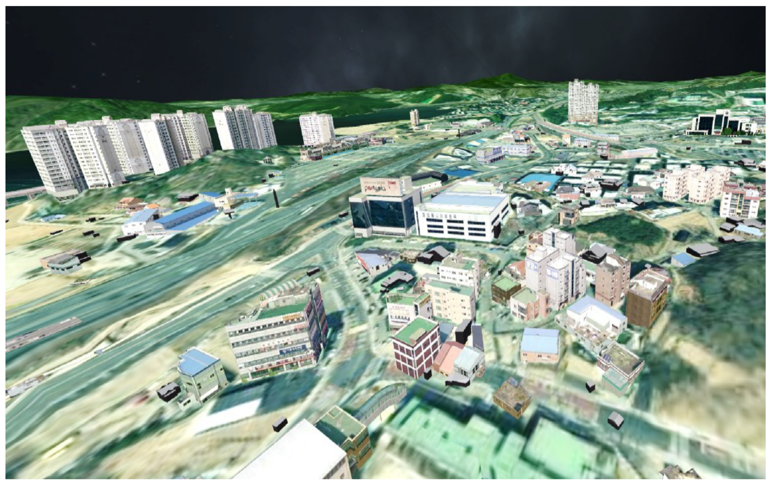
2.1. Data Generation and Characteristics

The 3D building models from VWorld were generated using a method where users manually match feature points on images [23]. As shown in Figure 2, when an operator visually identifies and selects the same points, such as a building corner, on two or more 2D images, the 3D spatial coordinates of that point are calculated using a projection matrix between the images. The user creates a 3D triangular mesh using at least three corresponding points on the same plane and then constructs a polygon mesh model that constitutes the entire building surface.

This approach differs from the typical 3D modeling approach that uses point clouds automatically generated through multi-view stereo (MVS) techniques [24]. While MVS automatically reconstructs camera positions, orientations, and the 3D structure of a scene from images, generating a dense point cloud, this method involves direct user intervention to select feature points and calculate 3D spatial coordinates. This approach allows for constructing 3D models at a relatively low cost without requiring specialized surveying equipment or expensive automated software. It is also advantageous for rapidly constructing a large number of building models, as even unskilled operators can relatively easily create 3D models. Through this method, the VWorld platform was able to build independent building models for the entire nation of South Korea in a short period. Unlike Google Earth’s digital surface model [25], which combines terrain and buildings, VWorld data have independent terrain models and building or facility models.

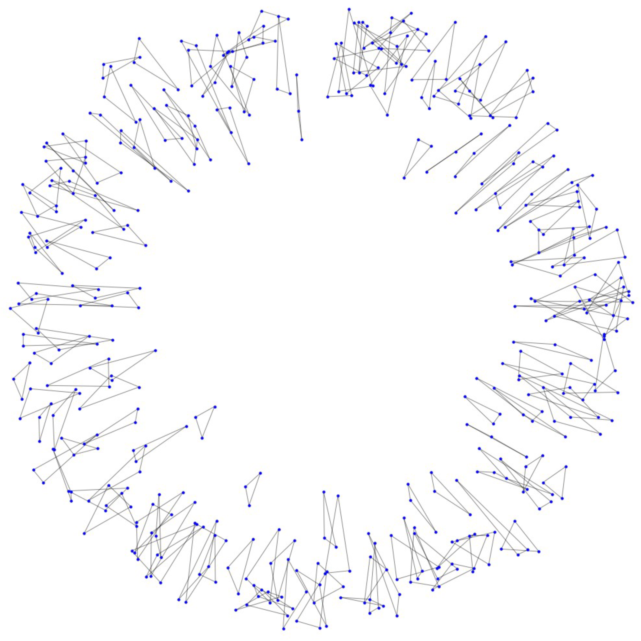
2.2. Data Limitations

The models used in this study have the following limitations, making efficient LoD generation through conventional mesh simplification [26,27] difficult. The generated 3D models are non-watertight or not watertight models. A watertight model is a closed model without gaps, clearly distinguishing between interior and exterior, and is generally represented as a solid model [28]. In contrast, the models used in this study often have holes or gaps, especially in areas like building floors, resulting in surfaces that are not entirely closed. This non-watertight characteristic fails to meet the input requirements (watertightness) of most mesh simplification algorithms [29].

Figure 3 presents a 3D model which is not a single object but rather multiple, discontinuously clustered polygons. Figure 4 then shows the graph data structure reconstructed from this 3D model. The 3D model’s vertices are transformed into graph nodes, and the edges into graph edges. This occurs due to the characteristics of the method where non-experts manually match feature points on images and create individual polygons without considering the model’s connectivity. Because of this, the problem of multiple vertices having the same or similar 3D spatial coordinates occurs frequently. Additionally, disconnectedness arises due to the non-topological structure, leading to geometrically unconnected or topologically inconsistent structures. In particular, even within a single object (e.g., one building), parts that should be composed of a single face are separated into multiple disconnected mesh clusters. When the vertices of the 3D model are converted to a graph model, the graph’s vertices should have unique identifiers [30]. However, in this model, multiple vertices exist at the same location, causing a single building to be composed of various disconnected graphs rather than a single connected graph. Consequently, FDCB leads to mesh quality degradation and simplification algorithms malfunctioning.

3. Methodology

This study presents a methodology for inspecting and refining the quality of 3D building models for UDT construction. The proposed method aims to enhance the reliability and usability of UDT data. The building model inspection and improvement process consists primarily of duplicate point removal and connected mesh clustering.

3.1. Duplicate Point Removal Methods

The FDCB data contain multiple vertices existing at nearly identical locations due to the characteristics of the modeling process. Detecting and removing these duplicate vertices is the first step in the model refinement process. This study proposes two methods for duplicate vertex removal: a vertex map approach and a k-dimensional tree (kd-tree) approach [31].

3.1.1. Vertex Map-Based Duplicate Removal

The vertex map-based duplicate vertex removal method uses the most intuitive solution of comparing distances between 3D coordinates and determining redundancy by calculating the distance between every point in the model and all other points. Specifically, for every point ${\mathbf{v}}_i$ in the 3D model, the Euclidean distance to every other point ${\mathbf{v}}_j$​ is calculated using the following equation:

$$d({\mathbf{v}}_i,{\mathbf{v}}_j)=\sqrt{{(x_i-x_j)}^2+{(y_i-y_j)}^2+{(z_i-z_j)}^2}$$

(1)

$$d({\mathbf{v}}_i,{\mathbf{v}}_j)<ϵ$$

(2)

If the computed distance d(${\mathbf{v}}_i$, ${\mathbf{v}}_j$) is less than or equal to a predefined threshold value, it is considered a duplicate point. Here, the threshold value $ϵ$ is set concerning the value used to determine identical points in commercial software such as the Unity engine. This may change depending on the data type used by each software. In the case of the Unity engine, $ϵ$ is set to ${10}^{-6}$. When a duplicate point is found, only one representative point is left, all points are removed, and all face information referencing the removed points is updated to refer to the remaining representative point to maintain data consistency. This method has the advantage of being very simple to implement, but since the distance must be calculated for all point pairs, the computational complexity becomes the square of the number of points, which may be inefficient for large-scale 3D models.

Algorithm 1 shows that it first traverses the original vertex array from the beginning and checks whether each vertex exists in the already registered vertex list. Specifically, it checks whether the current vertex is already recorded as index information in the $vertexMap$, and if not, it traverses the $uniqueVertices$ list to determine whether the same vertex exists. In this process, if two vertices are determined to be the same within the floating point error range, the existing vertex index is linked to the $vertexMap$ not to duplicate memory. On the other hand, if there is no identical vertex, a new vertex is added to $uniqueVertices$ and its location (index) is registered in the $vertexMap$. Even when UV or normal information is given, $uniqueUVs$ and $uniqueNormals$ are updated to refer to the same index to ensure consistent information between vertices.

After deduplication of the vertex array, each index in the triangle index array of the original mesh is converted through $vertexMap$ to construct a new triangle index array, $newTriangles$. At this time, since the index array is not proportional to the size of the vertex, it is stored by repeating the individual index sizes. Even if duplicates are removed, the size of the entire index array is the same. Through this, a vertex array without duplicates and a triangle index array updated to match the corresponding array are ultimately generated. The bounds and normal recalculation functions are called to organize the mesh if necessary. Since this algorithm goes through a nested comparison process, time complexity needs to be considered when the number of vertices is large, but if there are many duplicate vertices, it has the advantage of significantly reducing the memory usage and processing cost of the entire mesh.

Algorithm 1 Duplicate vertex removal algorithm using a vertex map

1: for $i\leftarrow 0$ to $length\left(\mathrm{originalVertices}\right)$ do   2:     $v_i\leftarrow \mathrm{originalVertices}\left[i\right]$   3:     if $i\notin \mathrm{vertexMap}$ then   4:         $isUnique\leftarrow \mathrm{TRUE}$   5:         for $j\leftarrow 0$ to $length\left(\mathrm{uniqueVertices}\right)$ do   6:            if IsEqual($v_i$, $\mathrm{uniqueVertices}\left[j\right]$) then   7:                $\mathrm{vertexMap}\left[i\right]\leftarrow j$   8:                $isUnique\leftarrow \mathrm{FALSE}$   9:                break 10:            end if 11:         end for 12:         if $isUnique=\mathrm{TRUE}$ then 13:            $\mathrm{vertexMap}\left[i\right]\leftarrow length\left(\mathrm{uniqueVertices}\right)$ 14:            $\mathrm{uniqueVertices}.\mathrm{add}\left(v_i\right)$ 15:            if $i<length\left(\mathrm{originalUVs}\right)$ then 16:                $\mathrm{uniqueUVs}.\mathrm{add}\left(\mathrm{originalUVs}\right[i\left]\right)$ 17:            end if 18:            if $i<length\left(\mathrm{originalNormals}\right)$ then 19:                $\mathrm{uniqueNormals}.\mathrm{add}\left(\mathrm{originalNormals}\right[i\left]\right)$ 20:            end if 21:         end if 22:     end if 23: end for 24: for $i\leftarrow 0$ to $length\left(\mathrm{originalTrianlges}\right)$ do 25:     $\mathrm{uniqueTriangles}.\mathrm{add}\left(\mathrm{vertexMap}\right[\mathrm{originalTriangles}\left[i\right]\left]\right)$ 26: end for

3.1.2. KD-Tree-Based Duplicate Removal

A kd-tree is a tree structure that partitions a high-dimensional space efficiently. Each node stores a pivot for a specific axis (dimension), and its child nodes belong to the left or right subtree according to that axis. For example, in a three-dimensional kd-tree, each node defines a partitioning plane. This partitioning plane is perpendicular to a specific axis (x, y, or z) and divides the space into two half-spaces based on the value of the axis (the partitioning pivot). When the partitioning axis of node N is d ($d\in \{x,y,z\}$) and the partitioning pivot is p, the left child node of N includes all points whose d-axis coordinates are less than p, and the right child node includes points greater than or equal to p. The following is a formula:

$$\begin{array}{cc}\hfill \mathrm{Left}\mathrm{Child}:& \{\mathbf{v}=(v_x,v_y,v_z)\mid v_d<p\}\hfill \end{array}$$

(3)

$$\begin{array}{cc}\hfill \mathrm{Right}\mathrm{Child}:& \{\mathbf{v}=(v_x,v_y,v_z)\mid v_d\ge p\}\hfill \end{array}$$

(4)

$\mathbf{v}$ is a vector representing a point in three-dimensional space. In the first split, the left and right are divided based on the x-coordinate; in the next level, the split is performed based on the y-coordinate; and in the level after that, the split is performed based on the z-coordinate. Since the space is divided alternately along a specific axis at each stage, the result is a hierarchical structure that recursively divides the space to which the data belong. The split criterion p is generally set to the median of the coordinate values ​​for the divided axis d among the points belonging to the corresponding node. Using the median helps maintain the tree’s balance, improving the search performance. Other methods include using the mean or selecting the point with the maximum variance, but the median is the most commonly used. Specifically, if node N has n points ${\mathbf{v}}_1,{\mathbf{v}}_2,\dots ,{\mathbf{v}}_n$ and the partitioning axis is d, then the d-axis coordinate values ​​$v_{1d},v_{2d},\dots ,v_{nd}$ of these points are sorted, and the median (if n is odd, the $(n+1)/2$nd value; if n is even, the average of the $n/2$nd and $(n/2)+1$st values) is set to p.

Using kd-tree, it can efficiently find the nearest neighbor to a specific point [32]. First, it builds a kd-tree that includes all points of the 3D model. Then, for each point ${\mathbf{v}}_i$, it finds all neighboring points ${\mathbf{v}}_j$ within a distance of $ϵ$ using the kd-tree. If such neighboring points exist, ${\mathbf{v}}_i$ and ${\mathbf{v}}_j$ are considered duplicate points, and all but one representative point are removed. The result of removing duplicate points is shown in Figure 5. Out of a total of 480 vertices, 407 are duplicated at 92 points. After removing duplicate vertices, a total of 73 single vertices are transformed. Using kd-tree, the time required to find the nearest neighbors of a given point increases logarithmically as the number of points (n) increases. Even if the number of points doubles, the search time increases by only 1 unit. The overall time complexity of the duplicate point removal task also tends to increase in the form $nlogn$ as the number of points increases. It makes the kd-tree-based method very efficient in removing duplicate points in large 3D models.

3.2. Spatial Partitioning-Based Connected Mesh Clustering

The 3D building model with duplicate points removed can still comprise several unconnected separate mesh clusters. This problem occurs when non-experts manually match feature points to reconstruct individual 3D polygons during the model creation. To utilize UDT, it is ideal for each building to be represented as a single object, i.e., a single connected mesh. Therefore, this study proposes a method to identify these separate mesh clusters and classify connected elements into a single mesh cluster by utilizing graph theory.

First, the 3D building model is converted into a graph model. Each vertex of the 3D model becomes a node of the graph, and each edge becomes an edge of the graph. Each node has a unique identifier and 3D spatial coordinates $(x,y,z)$. If an edge connects two vertices ${\mathbf{v}}_i$ and ${\mathbf{v}}_j$ in the 3D model, an edge connecting the corresponding nodes is also created in the graph model. Through this process, the 3D building model is expressed as an undirected graph $G=(V,E)$ where each vertex is a node and each edge is an edge. Here, V represents a set of nodes, and E represents a set of edges.

Once the graph model G is constructed, the connected mesh cluster is found using graph theory’s concept of connected components. A connected component refers to a set of reachable nodes connected through edges in the graph. To efficiently separate these components, it proposes a spatial partitioning-based Depth-First Search (DFS) algorithm, which improves over standard DFS. Algorithm 2 shows the pseudo-code of the proposed method.

Algorithm 2 Spatial partitioning-based DFS for connected mesh clustering

1: function AssignClusterIDs($graph,cell\_size$)   2:     $grid\leftarrow$CreateSpatialGrid($graph,cell\_size$)   3:     $node\_cluster\_map\leftarrow$ an empty dictionary   4:     $cluster\_id\leftarrow 0$   5:     for each $node$ in $graph$ do   6:         if $node\notin node\_cluster\_map$ then   7:            $cluster\_id\leftarrow cluster\_id+1$ DFS($graph,node,cluster\_id,node\_cluster\_map,grid$)   8:         end if   9:     end for 10:     return $node\_cluster\_map$ 11: end function 12: function DFS($graph,node,cluster\_id,node\_cluster\_map,grid$) 13:     $node\_cluster\_map\left[node\right]\leftarrow cluster\_id$ 14:     $x,y,z\leftarrow node.coordinates$ 15:     $i\leftarrow \lfloor (x-grid.bbox.min\_x)/grid.cell\_size\rfloor$ 16:     $j\leftarrow \lfloor (y-grid.bbox.min\_y)/grid.cell\_size\rfloor$ 17:     $k\leftarrow \lfloor (z-grid.bbox.min\_z)/grid.cell\_size\rfloor$ 18:     $cell\_index\leftarrow (i,j,k)$ 19:     for each $neighbor$ in $grid.cells[cell\_index]$do     ▹ only nodes in the same cell 20:         if $neighbor\notin node\_cluster\_map$ and $neighbor$ is a neighbor of $node$ in $graph$ then 21:            DFS($graph,neighbor,cluster\_id,node\_cluster\_map,grid$) 22:         end if 23:     end for 24: end function

The ‘AssignClusterIDs’ function takes a graph G and a cell size $cell\_size$ as input and assigns a connected cluster ID to each node. First, it calls the ‘CreateSpatialGrid’ function to divide the 3D space into a grid and assigns each node to the corresponding grid cell. The ‘CreateSpatialGrid’ function first calculates the bounding box of the 3D model using the ‘CalculateBoundingBox’ function in Algorithm 3. Then, it initializes the ‘SpatialGrid’ object. The ‘SpatialGrid’ function has a dictionary type cells, and each cell stores the nodes belonging to the cell in the form of a list. The ‘AssignClusterIDs’ function traverses all the nodes in the graph, assigns a new cluster ID to any node that has not yet been assigned a cluster ID, and calls the ‘DFS’ function starting from that node. The ‘DFS’ function recursively searches the neighboring nodes that belong to the same cell as the current node and assigns them the same cluster ID. At this time, a condition is added to check whether the two nodes are connected in the graph ($neighbor$ is a neighbor of $node$ in $graph$) to prevent incorrect clustering.

Algorithm 3 Creationof the spatial grid

1: function CreateSpatialGrid($graph,cell\_size$)   2:     $bbox\leftarrow$CalculateBoundingBox($graph$)   3:     $grid\leftarrow$ a new SpatialGrid   4:     $grid.cell\_size\leftarrow cell\_size$   5:     $grid.bbox\leftarrow bbox$   6:     for each $node$ in $graph$ do   7:         $x,y,z\leftarrow node.coordinates$   8:         $i\leftarrow \lfloor (x-bbox.min\_x)/cell\_size\rfloor$   9:         $j\leftarrow \lfloor (y-bbox.min\_y)/cell\_size\rfloor$ 10:         $k\leftarrow \lfloor (z-bbox.min\_z)/cell\_size\rfloor$ 11:         $cell\_index\leftarrow (i,j,k)$ 12:         if $cell\_index$ not in $grid.cells$ then 13:            $grid.cells[cell\_index]\leftarrow$ an empty list 14:         end if 15:         $grid.cells[cell\_index].append\left(node\right)$ 16:     end for 17:     return $grid$ 18: end function 19: function CalculateBoundingBox($graph$) 20:     $bbox\leftarrow$ a new BoundingBox 21:     for each $node$ in $graph$ do 22:         $x,y,z\leftarrow node.coordinates$ 23:         for all $coord\in \{x,y,z\}$ do 24:            $bbox.min\_coord\leftarrow min(bbox.min\_coord,coord)$ 25:            $bbox.max\_coord\leftarrow max(bbox.max\_coord,coord)$ 26:         end for 27:     end for 28:     return $bbox$ 29: end function

The core of this algorithm is to reduce unnecessary operations by limiting the DFS search range through space partitioning. To do this, the 3D space is divided into cells, and only the nodes belonging to each cell are considered neighbors. The cell size ($cell\_size$) is a parameter that significantly affects the algorithm’s performance. The cell size is automatically determined based on the bounding box of the 3D model. First, the bounding box is calculated using the coordinates of all vertices of the 3D model. After calculating the diagonal length ($diag\_length$) of the bounding box, it is divided by the $factor$ value to determine the cell size.

$$cell\_size={\displaystyle \frac{diag\_length}{factor}}$$

(5)

$$diag\_length=\sqrt{{(max\_x-min\_x)}^2+{(max\_y-min\_y)}^2+{(max\_z-min\_z)}^2}$$

(6)

($min\_x,min\_y,min\_z$) and ($max\_x,max\_y,max\_z$) are the minimum and maximum coordinate values ​​of the bounding box, respectively. The factor value is automatically determined based on the node density of the 3D model. First, $volume$ of the bounding box is calculated. Here, N is the total number of nodes in the 3D model.

$$volume=(max\_x-min\_x)\ast (max\_y-min\_y)\ast (max\_z-min\_z)$$

(7)

$$density={\displaystyle \frac{N}{volume}}$$

(8)

$$factor=base\_factor\times \left({\displaystyle \frac{1}{1+{log}_{10}(1+density)}}\right)$$

(9)

As can be seen in the Equation (9), the higher the node density, the smaller the $factor$ value, and consequently, the smaller the cell size ($cell\_size$). Conversely, the lower the node density, the larger the $factor$ value, and the larger the cell size. Here, $base\_factor$ is a basic value set by the user, and an appropriate value can be selected through experiments. In this study, $base\_factor$ was set to 10. Here, $base\_factor$ is a parameter that determines the basic scale of the cell size. In this study, $base\_factor$ was set to 10 based on preliminary experiments. It means a cell size corresponding to approximately 1/10 of the bounding box’s diagonal length, which is considered large enough to separate different buildings without separating small structures inside the building in a general building model. However, the $base\_factor$ value may vary depending on the characteristics of the data (e.g., building density, size distribution).

The proposed method separates a 3D model composed of independent polygons into several connected mesh clusters. This spatial partitioning-based approach effectively addresses the non-connectivity problem in 3D building models. Figure 6 visualizes the resulting connected graph after applying duplicate vertex removal and spatial partitioning-based DFS to the model in Figure 4.

4. Experimental Results and Discussion

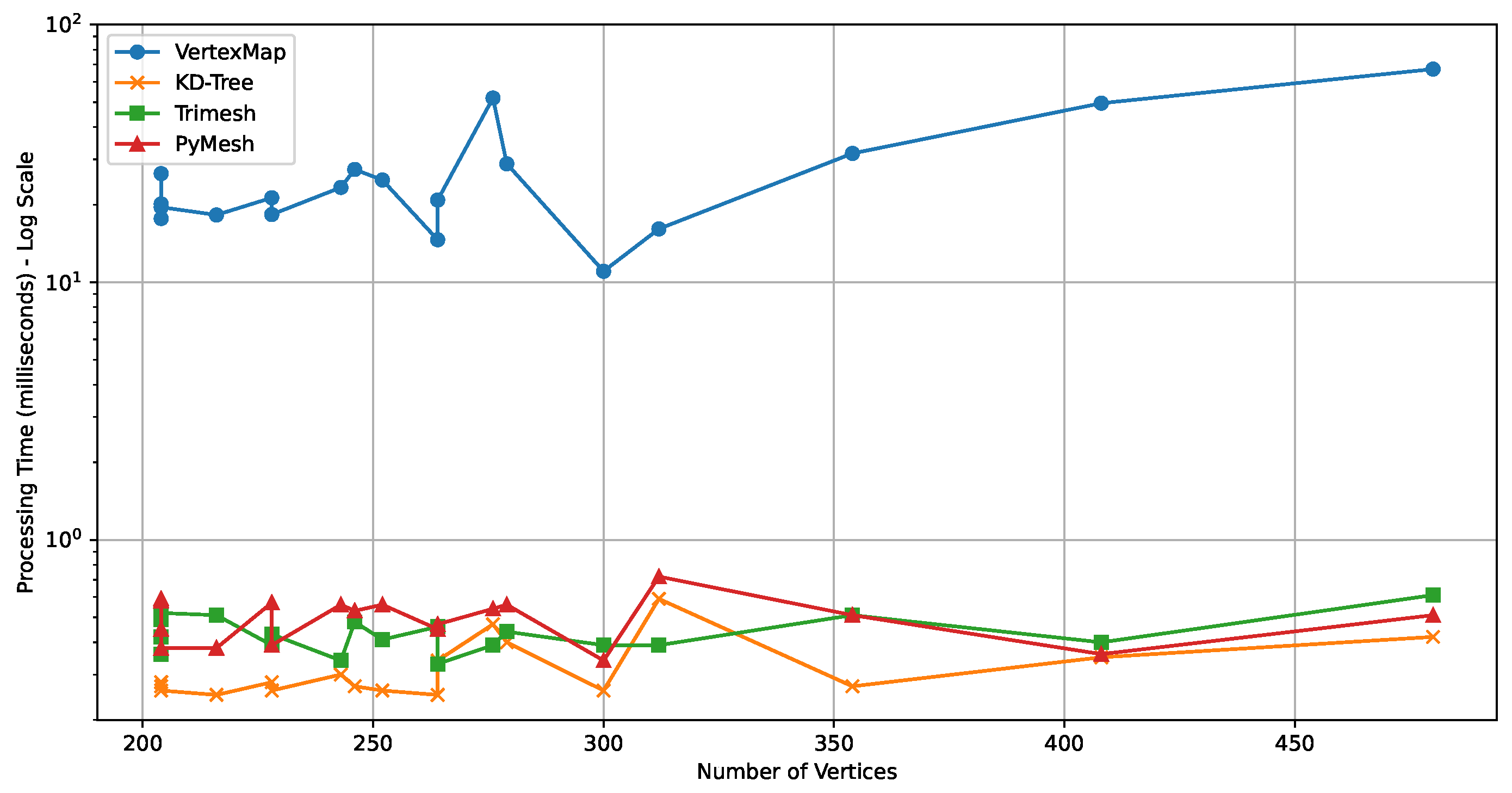
4.1. Experimental Results of Duplicate Point Removal Methods

This study compared the performance of the vertex map and the kd-tree methods for removing duplicate vertices. Furthermore, a comparison was made with the duplicate point removal functions of Trimesh [33] and PyMesh [34], which are widely used 3D model processing libraries. Experiments were conducted on 20 3D building models of various sizes and complexities. The duplicate vertex removal ratio and execution speed of each method were measured, and the results are presented in

Table 1. Comparison of processing times (ms) for duplicate point removal across various methods: vertexMap, kd-Tree, Trimesh, PyMesh.

Number of Vertices	Vertices After Removal	Ratio (%)	Processing Time (ms)
			Vertex Map	KD-Tree	Trimesh	PyMesh
480	73	15.2	67.21	0.42	0.61	0.51
354	82	23.2	49.55	0.35	0.40	0.36
312	78	25.0	31.63	0.27	0.51	0.51
216	50	23.1	16.11	0.59	0.39	0.72
204	50	24.5	11.03	0.26	0.39	0.34
300	72	24.0	28.83	0.40	0.44	0.56
408	96	23.5	51.90	0.47	0.39	0.54
204	44	21.6	14.24	0.27	0.41	0.66
204	50	24.5	13.70	0.28	0.35	0.30
204	58	28.4	14.62	0.25	0.46	0.45
228	60	26.3	20.85	0.34	0.33	0.47
276	56	20.3	24.94	0.26	0.41	0.56
276	70	25.4	27.41	0.27	0.48	0.53
252	62	24.6	23.34	0.30	0.34	0.56
279	60	21.5	21.28	0.28	0.39	0.57
246	66	26.8	18.32	0.26	0.43	0.39
243	58	23.9	18.25	0.25	0.51	0.38
228	60	26.3	17.68	0.28	0.36	0.45
264	66	25.0	20.14	0.28	0.42	0.58
264	60	22.7	26.41	0.27	0.49	0.59

. The building data model provided by the VWorld Spatial Information Open Platform [23] was used for the experiments.

As a result of the experiment, as shown in Figure 7, the kd-tree-based method shows the fastest speed overall, and Trimesh and PyMesh also show relatively good performance. This is because kd-tree uses a data structure that recursively divides the 3D space and hierarchically organizes points. Trimesh uses a hashing technique, and PyMesh internally divides the space through voxelization to reduce the search range for duplicate points. On the other hand, the vertex map-based method implemented in this study shows a relatively slow speed because the distances between all point pairs have to be compared. However, the vertex map method has the advantage of being easy to implement in the Unity environment without a separate external library. During the duplicate vertex removal process, it can directly manage and control the mapping information between the original vertex and the new vertex.

In terms of the duplicate point removal ratio, all methodologies showed similar levels of performance, which is interpreted as being because most of the criteria for judging duplicate points are the same. In conclusion, for large-scale UDT building model data processing, it is advantageous to use efficient data structures and algorithms such as kd-tree, Trimesh, and PyMesh. However, when the model size is small, real-time processing is essential, and additional vertex attribute information (UV, normal vectors, etc.) must be processed together, the vertex map-based method implemented in this study can also be a helpful alternative.

4.2. Experimental Results of Mesh Clustering Using Spatial DFS

The experiments were conducted to verify the accuracy and efficiency of the proposed spatial partitioning-based DFS connected graph verification algorithm. For comparison, the widely used graph traversal algorithms, standard DFS, breadth-first search (BFS), and Union-Find algorithm, were additionally implemented, and their performance was compared. BFS is a breadth-first search algorithm that traverses the graph by sequentially visiting nodes closest to the starting node [35]. While DFS explores one path as deeply as possible before exploring the next, BFS explores the graph breadth-wise, starting from the nodes closest to the start node. The Union-Find algorithm utilizes the disjoint set data structure to manage the connected components of a graph efficiently and is particularly useful for connectivity determination in dynamic graph environments [36].

Since the VWorld 3D building models, which are the target data of this paper, do not have a ground truth for disconnected graph models, 100 data sets were randomly generated for the experiment. Each data set has 500 points with x, y, and z coordinates ranging from −100 to 100. Each data set was randomly generated with one to five connected graphs, allowing us to measure the accuracy of connected graph identification when evaluating the algorithms. Using the generated data set, the proposed spatial DFS and the comparative methods such as standard DFS, BFS, and Union-Find algorithms were each executed, and accuracy and execution times were measured.

As shown in

Table 2. Comparison of accuracy and average execution time for graph connectivity verification using DFS, spatial DFS, BFS, and Union-Find on 100 data sets.

Algorithm	Accuracy (%)	Average Time (ms)
DFS	100	164.63
Spatial DFS	100	23.96
BFS	100	415.64
Union-Find	100	162.12

, all four methods achieve 100% accuracy in ideally determining all graphs’ connectivity. The execution time of the proposed spatial DFS is the fastest. This demonstrates that the proposed spatial DFS algorithm can perform connectivity verification with high reliability and speed across various graph structures. Notably, the comparative algorithms, standard DFS, BFS, and Union-Find, also exhibit high accuracy. However, the Union-Find algorithm may be more suitable in dynamic graph environments where nodes or edges of the graph model are frequently added or deleted in real-time. This is because it only requires updating the relevant portions of the data structure instead of re-traversing the entire graph for modifications.

Figure 8 shows the execution times for individual data sets. For spatial DFS, each data set’s cell size is calculated using the method proposed in Section 3.2. The average cell size across the 100 data sets is 34.5. The experimental results show that the proposed spatial DFS method generally exhibits faster execution times. Spatial DFS records execution times of less than 50 ms for most data sets, demonstrating stable performance. This is because the spatial partitioning technique effectively reduces the search space by minimizing unnecessary distance calculations. This experiment showed that spatial DFS is more efficient than other methods when performing connectivity analysis of point data in 3D space. The benefits of spatial partitioning are particularly pronounced when the data density is low, and the threshold distance is relatively small. These results suggest the potential applicability of the spatial partitioning-based DFS algorithm in various applications, including large-scale 3D data processing (e.g., point clouds, molecular structures) and network analysis.

Figure 9 is an example of a rendered 3D building model after removing duplicate points and partitioning it into connected mesh clusters. The building model, which was initially composed of multiple independent polygons, is transformed into a model consisting of three connected mesh clusters through the proposed method. The individual mesh clusters of the building, derived through the proposed method, can be modified according to the purpose.

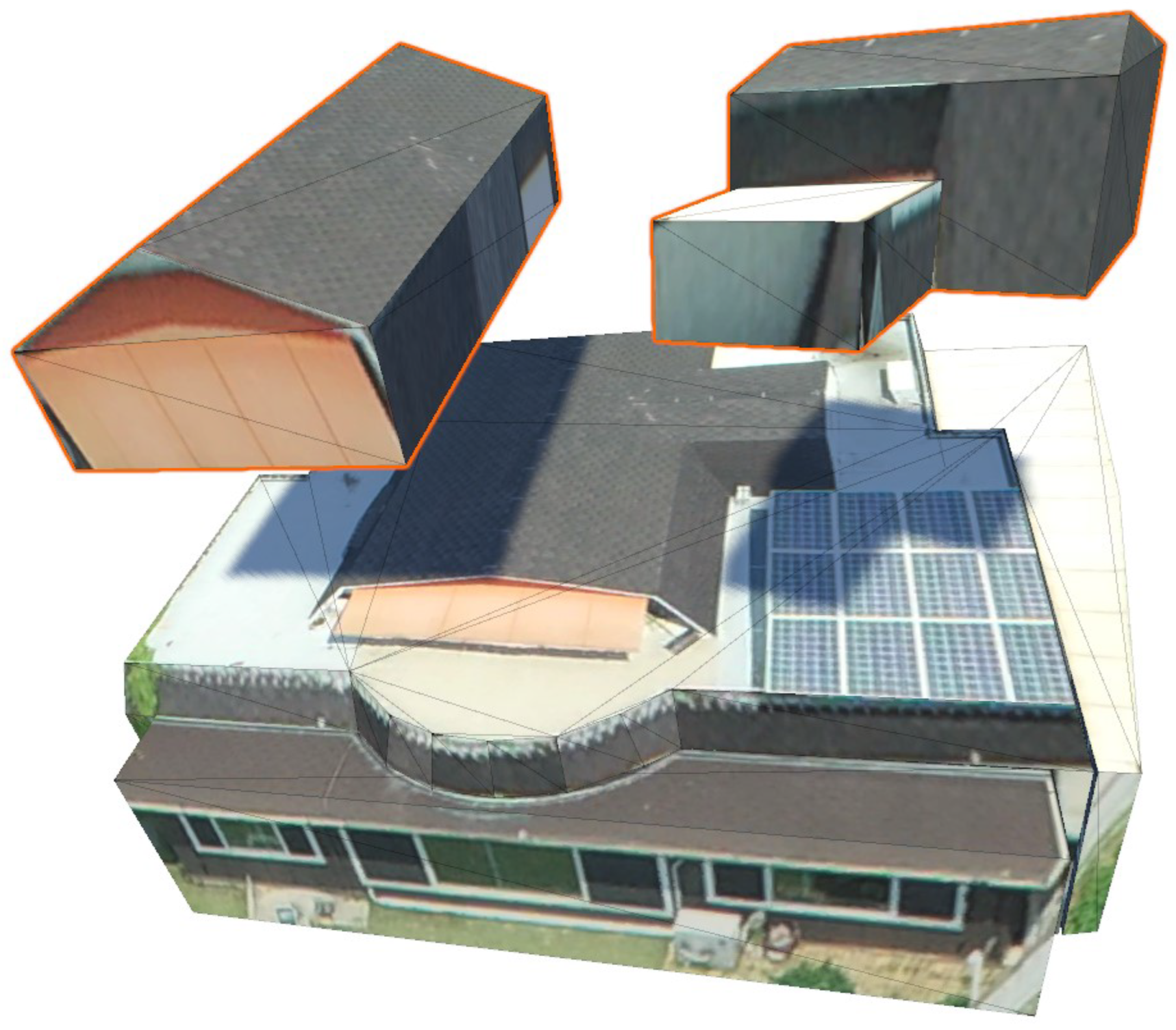
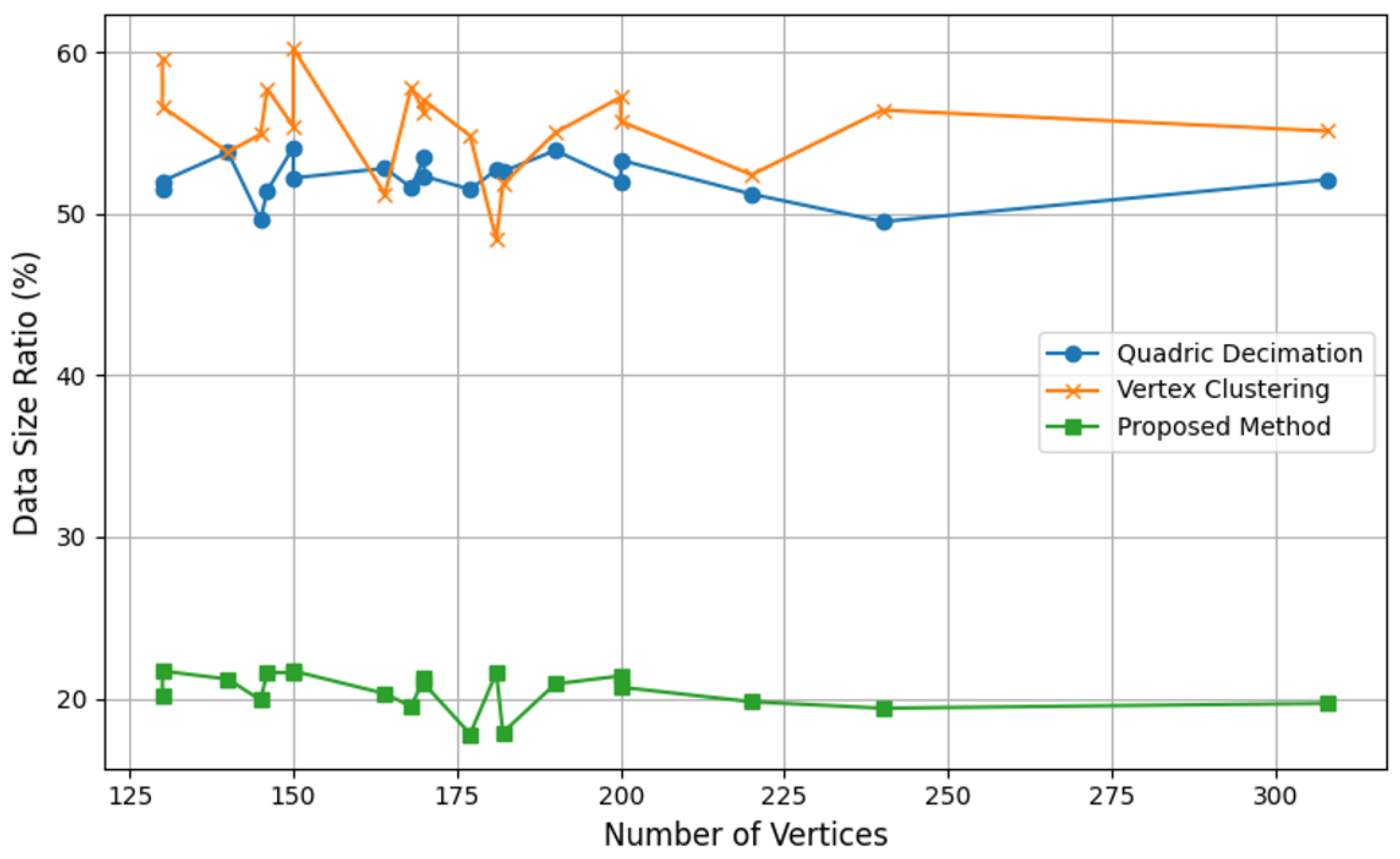
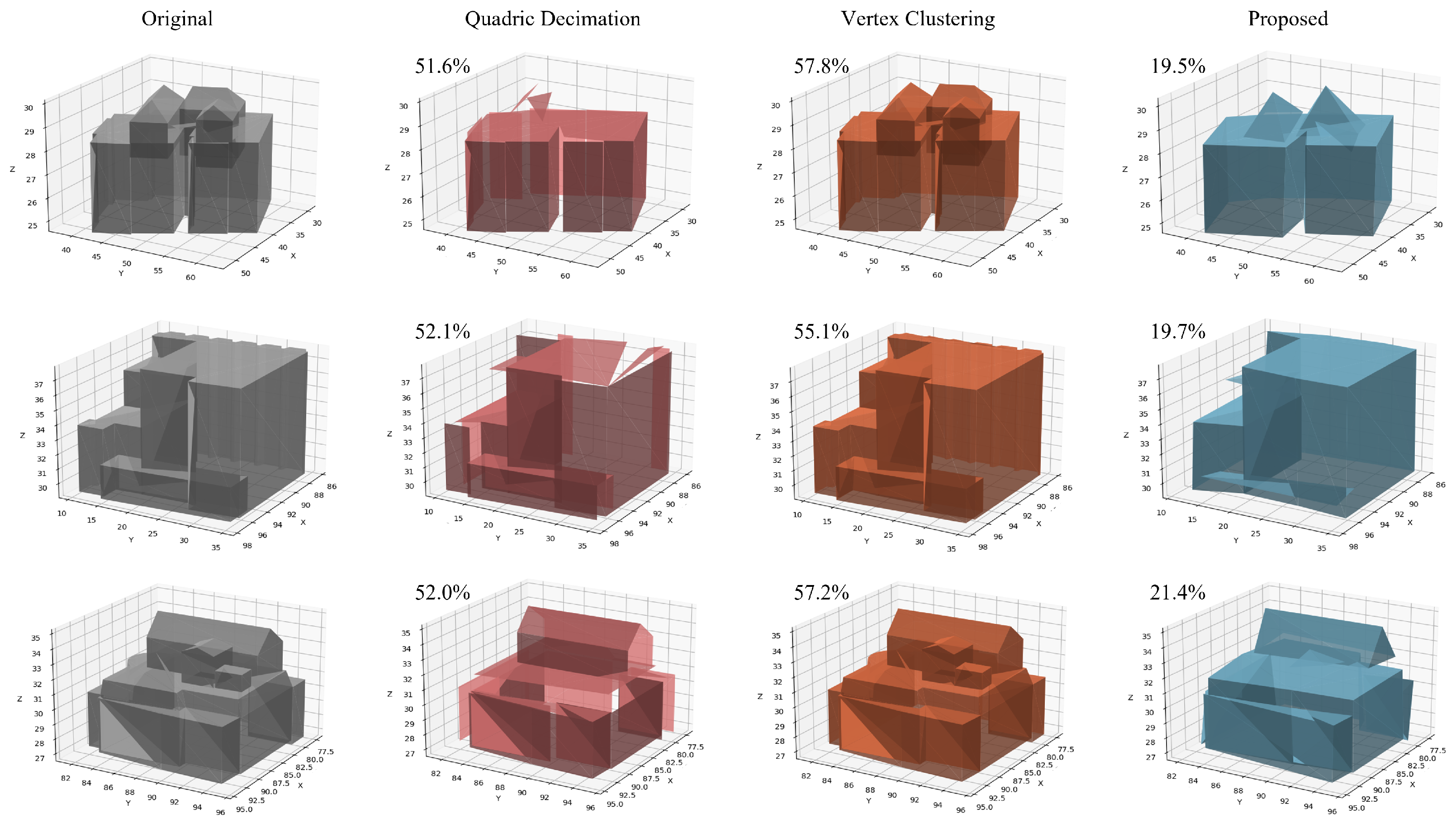
4.3. Comparative Evaluation of Mesh Simplification

Two widely used algorithms, Quadric Decimation [37] and Vertex Clustering [38], were compared to evaluate their impact on data ratios resulting from mesh simplification for LoD construction. Quadric Decimation is a method that simplifies meshes by iteratively merging pairs of vertices that minimize error, thus preserving the shape’s features relatively well. Vertex Clustering divides the space into a voxel grid and merges the vertices within each voxel into a single representative vertex, performing a relatively uniform simplification. The experiment was conducted using the Open3D library [39]. For each model, the number of vertices and triangles in the original mesh and the corresponding counts after simplification using the three methods were measured. The building data models provided by the VWorld spatial information open platform were used to perform the experiment [23]. The proposed method applies Quadric Decimation to the result of classifying connected mesh clusters using kd-tree-based duplicate vertex removal and spatial DFS.

Table 3. Mesh simplification results: comparison of Quadric Decimation, Vertex Clustering, and proposed methods.

Original		Quadric Decimation		Vertex Clustering		Proposed Method
Vertex	Triangles	Vertex	Triangles	Vertex	Triangles	Vertex	Triangles
164	82	106	24	50	76	26	24
146	76	92	22	52	76	26	22
145	81	88	24	52	72	21	24
170	84	111	25	59	84	30	24
177	93	112	27	55	93	22	26
181	92	117	27	48	84	33	26
200	104	127	31	70	104	34	31
200	100	130	30	67	100	32	30
220	118	138	35	71	106	32	35
182	92	117	27	54	88	22	27
190	92	125	27	63	92	33	26
168	88	106	26	60	88	24	26
150	72	99	21	51	72	27	21
150	76	96	22	60	76	27	22
130	68	82	20	50	68	21	19
308	160	196	48	98	160	44	48
140	68	92	20	44	68	24	20
170	88	109	26	62	85	29	25
130	68	83	20	47	65	24	19
240	136	146	40	85	127	34	39

presents the detailed numerical results of the experiment. The proposed method generates meshes with significantly fewer vertices and triangles than Quadric Decimation and Vertex Clustering, consistently achieving a higher level of simplification. This reduction in complexity is effective for applications with limited computing resources or those requiring real-time processing. The data size ratio, calculated as the number of vertices in the simplified mesh divided by the number of vertices in the original mesh, is visualized in Figure 10. This graph visually confirms the superior compression ratio of the proposed method. Across the range of models tested, the proposed method consistently maintains a data size ratio below 25%, while Quadric Decimation and Vertex Clustering exhibit considerably higher ratios.

Figure 11 visually compares the mesh simplification results using the proposed method, Quadric Decimation, and Vertex Clustering. Compared to the Quadric Decimation and Vertex Clustering methods, the proposed method generally achieves the lowest data size ratio (%), confirming its highest mesh simplification efficiency. This suggests that the proposed method effectively improves the problems of discontinuous building models by removing duplicate vertices and classifying connected mesh clusters.

While the proposed method exhibits the best performance in data size ratio, each method shows different characteristics in preserving the appearance of the simplified mesh. Quadric Decimation excludes building surfaces or small external mesh clusters compared to the proposed method. In contrast, Vertex Clustering shows results that best preserve the building’s outer shape. These results indicate that each method can be suitably utilized for different levels of LoD when constructing the LoD of a building model. Optimal results can be expected according to the application purpose and requirements, such as using the Vertex Clustering method when the camera is relatively close to the building and using the proposed method when the camera is far away and only a simplified building shape is required.

4.4. Discussion

This study holds significance in that it detects geometric and topological errors in 3D building models, a core component of UDT, and improves the overall quality of UDT data by refining the models. In particular, considering the characteristics of large-scale 3D building models created by unskilled workers, which were overlooked in previous studies, a method was presented to solve problems such as duplicate points and disconnections effectively. This will reduce errors cause by manual work, increase work efficiency, and save time and cost in constructing large-scale, city-level UDTs.

However, this study has some limitations, and there are tasks that need to be addressed in future research. The current methodology performs up to the step of classifying connected mesh clusters but does not include the function of automatically merging multiple clusters belonging to the same building. In the future, it is necessary to develop a more accurate and efficient cluster merging algorithm by comprehensively utilizing geometric features such as distance between clusters, normal vector similarity, area/volume ratio, and attribute information such as building ID. In addition, this study focused on geometric and topological error checking and did not consider semantic error checking. For example, research has not been conducted to check and correct semantically incorrect models, such as when a window is floating outside the wall. In future research, it is necessary to develop a higher-level error checking and correction method by utilizing the semantic information of the building model.

This study focused on explaining the concept and operation of the proposed algorithm, as well as providing a detailed performance evaluation. Future research should evaluate the performance of the algorithm on real UDT data of various sizes and complexities and improve the efficiency of the algorithm by applying various optimization techniques such as parallel processing and GPU acceleration. In addition, research is needed on developing an LoD generation algorithm using the refined model and a method to integrate it into a real UDT system to inspect and refine model quality in real time.

5. Conclusions

This study proposed a method for improving the geometric and topological correction of 3D building models used to construct urban digital twins (UDTs). It consists of geometric refinement through duplicate point removal and topological refinement through connected mesh clustering for 3D building models with FDCB problems. Efficient algorithms are applied at each stage to detect and correct geometric and topological errors in the model. In particular, a spatial partitioning-based DFS method was proposed to analyze the topological connectivity of 3D models, and the FDCB problems were effectively solved. This study is expected to improve the reliability and accuracy of UDT data, expanding their applicability in various applications (LoD generation, 3D printing, simulation, structural analysis, etc.). Refined, high-quality 3D building models will play a key role in various UDT-based services, providing more accurate and reliable analysis results.

In future research, this methodology will be further developed to enhance geometric and topological refinement functions by automatically merging multiple clusters belonging to the same building and converting non-watertight models to watertight models. To this end, algorithms that utilize geometric features such as distance between clusters and normal vector similarity, attribute information such as building IDs, and algorithms that automatically fill gaps or holes in non-watertight models will be developed. Future studies are expected to advance the technology for inspecting and refining the geometric and topological accuracy of 3D building models, apply it in real-world UDT systems, and contribute to solving urban problems and improving the quality of life for citizens.

References

1. Lee, A.; Lee, K.W.; Kim, K.H.; Shin, S.W. A geospatial platform to manage large-scale individual mobility for an urban digital twin platform. Remote Sens. 2022, 14, 723. [Google Scholar] [CrossRef]
2. Gröger, G.; Plümer, L. CityGML–Interoperable semantic 3D city models. ISPRS J. Photogramm. Remote. Sens. 2012, 71, 12–33. [Google Scholar] [CrossRef]
3. Yu, D.; Ji, S.; Liu, J.; Wei, S. Automatic 3D building reconstruction from multi-view aerial images with deep learning. ISPRS J. Photogramm. Remote. Sens. 2021, 171, 155–170. [Google Scholar] [CrossRef]
4. Ren, Y.; Li, X.; Jin, F.; Li, C.; Liu, W.; Li, E.; Zhang, L. Extracting Regular Building Footprints Using Projection Histogram Method from UAV-Based 3D Models. ISPRS Int. J.-Geo-Inf. 2024, 14, 6. [Google Scholar] [CrossRef]
5. Gorelick, N.; Hancher, M.; Dixon, M.; Ilyushchenko, S.; Thau, D.; Moore, R. Google Earth Engine: Planetary-scale geospatial analysis for everyone. Remote. Sens. Environ. 2017, 202, 18–27. [Google Scholar] [CrossRef]
6. Lee, A. A Camera Control Method for a Planetary-Scale 3D Map based on a Game Engine with Floating Point Precision Limitation. IEEE Access 2024, 12, 100240–100250. [Google Scholar] [CrossRef]
7. Tyagi, N.; Singh, J.; Singh, S.; Sehra, S.S. A 3D Model-Based Framework for Real-Time Emergency Evacuation Using GIS and IoT Devices. ISPRS Int. J.-Geo-Inf. 2024, 13, 445. [Google Scholar] [CrossRef]
8. Gao, R.; Yan, G.; Wang, Y.; Yan, T.; Niu, R.; Tang, C. Construction of a Real-Scene 3D Digital Campus Using a Multi-Source Data Fusion: A Case Study of Lanzhou Jiaotong University. ISPRS Int. J.-Geo-Inf. 2025, 14, 19. [Google Scholar] [CrossRef]
9. Verma, V.; Kumar, R.; Hsu, S. 3D building detection and modeling from aerial LIDAR data. In Proceedings of the 2006 IEEE Computer Society Conference on Computer Vision and Pattern Recognition (CVPR’06), New York, NY, USA, 17–22 June 2006; IEEE: New York, NY, USA, 2006; Volume 2, pp. 2213–2220. [Google Scholar]
10. Müller, P.; Zeng, G.; Wonka, P.; Van Gool, L. Image-based procedural modeling of facades. ACM Trans. Graph. 2007, 26, 85. [Google Scholar] [CrossRef]
11. Jiang, Y.; Dai, Q.; Min, W.; Li, W. Non-watertight polygonal surface reconstruction from building point cloud via connection and data fit. IEEE Geosci. Remote. Sens. Lett. 2021, 19, 1–5. [Google Scholar] [CrossRef]
12. Skrzypczak, I.; Oleniacz, G.; Leśniak, A.; Zima, K.; Mrówczyńska, M.; Kazak, J.K. Scan-to-BIM method in construction: Assessment of the 3D buildings model accuracy in terms inventory measurements. Build. Res. Inf. 2022, 50, 859–880. [Google Scholar] [CrossRef]
13. Lo, S. A new mesh generation scheme for arbitrary planar domains. Int. J. Numer. Methods Eng. 1985, 21, 1403–1426. [Google Scholar] [CrossRef]
14. George, P.; Borouchaki, H.; Laug, P. An efficient algorithm for 3D adaptive meshing. Adv. Eng. Softw. 2002, 33, 377–387. [Google Scholar] [CrossRef]
15. Cignoni, P.; Callieri, M.; Corsini, M.; Dellepiane, M.; Ganovelli, F.; Ranzuglia, G. Meshlab: An open-source mesh processing tool. In Proceedings of the Eurographics Italian Chapter Conference, Salerno, Italy, 2–4 July 2008; Volume 2008, pp. 129–136. [Google Scholar]
16. Shewchuk, J.R. Delaunay refinement algorithms for triangular mesh generation. Comput. Geom. 2002, 22, 21–74. [Google Scholar] [CrossRef]
17. Biljecki, F.; Ledoux, H.; Du, X.; Stoter, J.; Soon, K.H.; Khoo, V. The most common geometric and semantic errors in CityGML datasets. In Proceedings of the ISPRS Annals of the Photogrammetry, Remote Sensing and Spatial Information Sciences, Athens, Greece, 20–21 October 2016; Volume IV-2/W1. [Google Scholar]
18. Rashidan, H.; Abdul Rahman, A.; Musliman, I.A.; Buyuksalih, G. Triangular mesh approach for automatic repair of missing surfaces of lod2 building models. Int. Arch. Photogramm. Remote. Sens. Spat. Inf. Sci. 2022, 46, 281–286. [Google Scholar] [CrossRef]
19. Ju, T. Fixing geometric errors on polygonal models: A survey. J. Comput. Sci. Technol. 2009, 24, 19–29. [Google Scholar] [CrossRef]
20. Shewchuk, J.R. Triangle: Engineering a 2D quality mesh generator and Delaunay triangulator. In Proceedings of the Workshop on Applied Computational Geometry, Philadelphia, PA, USA, 27–28 May 1996; Springer: Berlin/Heidelberg, Germany, 1996; pp. 203–222. [Google Scholar]
21. Tautges, T.J.; Blacker, T.; Mitchell, S.A. The whisker weaving algorithm: A connectivity-based method for constructing all-hexahedral finite element meshes. Int. J. Numer. Methods Eng. 1996, 39, 3327–3349. [Google Scholar] [CrossRef]
22. Ministry of Land, Infrastructure and Transport Spatial Information Industry Promotion Institute. VWorld. 2025. Available online: https://www.vworld.kr/v4po_main.do (accessed on 25 February 2025).
23. Lee, A.; Jang, I. Implementation of an open platform for 3D spatial information based on WebGL. ETRI J. 2019, 41, 277–288. [Google Scholar] [CrossRef]
24. Hartley, R.; Zisserman, A. Multiple View Geometry in Computer Vision; Cambridge University Press: Cambridge, UK, 2003. [Google Scholar]
25. Chen, J.; Clarke, K.C.; Freundschuh, S. Rapid 3d modeling using photogrammetry applied to google earth. In Proceedings of the 19th International Research Symposium on Computer-Based Cartography Albuquerque. Cartography and Geographic Information Society, Albuquerque, NM, USA, 14–16 September 2016; pp. 14–16. [Google Scholar]
26. GharehTappeh, Z.S.; Peng, Q. Simplification and unfolding of 3D mesh models: Review and evaluation of existing tools. Procedia CIRP 2021, 100, 121–126. [Google Scholar] [CrossRef]
27. Li, Z.; Zhao, Z.; Gao, W.; Jiao, L. An Algorithm for Simplifying 3D Building Models with Consideration for Detailed Features and Topological Structure. ISPRS Int. J.-Geo-Inf. 2024, 13, 356. [Google Scholar] [CrossRef]
28. Cai, Y.; Fan, L. An efficient approach to automatic construction of 3D watertight geometry of buildings using point clouds. Remote. Sens. 2021, 13, 1947. [Google Scholar] [CrossRef]
29. Sade, B.; Oya, S.; Lee, J.H. Non-watertight dural reconstruction in meningioma surgery: Results in 439 consecutive patients and a review of the literature. J. Neurosurg. 2011, 114, 714–718. [Google Scholar] [CrossRef] [PubMed]
30. Bondy, J.A.; Murty, U.S.R. Graph Theory; Springer Publishing Company, Incorporated: Princeton, NJ, USA, 2008. [Google Scholar]
31. Virtanen, P.; Gommers, R.; Oliphant, T.E.; Haberland, M.; Reddy, T.; Cournapeau, D.; Burovski, E.; Peterson, P.; Weckesser, W.; Bright, J.; et al. SciPy 1.0: Fundamental Algorithms for Scientific Computing in Python. Nat. Methods 2020, 17, 261–272. [Google Scholar] [CrossRef] [PubMed]
32. Ram, P.; Sinha, K. Revisiting kd-tree for nearest neighbor search. In Proceedings of the 25th Acm Sigkdd International Conference on Knowledge Discovery & Data Mining, Anchorage, AK, USA, 4–8 August 2019; pp. 1378–1388. [Google Scholar]
33. Dawson-Haggerty Trimesh. 2019. Available online: https://trimesh.org/ (accessed on 28 February 2025).
34. Zhou, Q. PyMesh: Geometry Processing Library for Python. 2016. Available online: https://pymesh.readthedocs.io/ (accessed on 28 February 2025).
35. Cormen, T.H.; Leiserson, C.E.; Rivest, R.L.; Stein, C. Introduction to Algorithms; MIT Press: Cambridge, MA, USA, 2022. [Google Scholar]
36. Sedgewick, R.; Wayne, K. Algorithms; Addison-Wesley Professional: Boston, MA, USA, 2011. [Google Scholar]
37. Garland, M.; Heckbert, P.S. Surface simplification using quadric error metrics. In Proceedings of the 24th Annual Conference on Computer Graphics and Interactive Techniques, Los Angeles, CA, USA, 3–8 August 1997; pp. 209–216. [Google Scholar]
38. Weibel, R.; Burgardt, D.; Shashi, S.; Hui, X. On-the-Fly Generalization; Springer: Berlin/Heidelberg, Germany, 2008; pp. 339–344. [Google Scholar]
39. Zhou, Q.Y.; Park, J.; Koltun, V. Open3D: A modern library for 3D data processing. arXiv 2018, arXiv:1801.09847. [Google Scholar]
Figure 1. Visualization of the UDT model. A 3D GIS, developed using the Unity3D engine, was implemented in this study for UDT visualization.
Ijgi 14 00198 g001
Figure 2. 3D building reconstruction from multi-temporal aerial images. Corresponding points on a planar building faces (highlighted in red) are manually selected in both images from times t and t + 1 to define a polygon for model reconstruction.
Ijgi 14 00198 g002
Figure 3. Example of a VWorld 3D building model with the FDCB issue.
Ijgi 14 00198 g003
Figure 4. Graph representation of the 3D model in Figure 3, where 3D model vertices are represented as graph nodes and 3D model edges are graph edges. The structure reveals multiple disconnected meshes and polygon clusters due to FDCB issues. The graph has 480 nodes and 480 edges.
Ijgi 14 00198 g004
Figure 5. Result of duplicate vertex search using the kd-tree on the 3D model of Figure 4, showing the removal of 407 duplicate points out of 480 total points.
Ijgi 14 00198 g005
Figure 6. Example of a connected graph model representing the connected mesh components of a 3D building model. The original disconnected model (in Figure 4) initially contained 480 nodes and 480 edges. After removing duplicate vertices and applying the proposed spatial partitioning-based DFS algorithm to identify connected components, the graph model is composed of 73 unique vertices nodes and 204 edges.
Ijgi 14 00198 g006
Figure 7. Comparison of processing times (log scale) for duplicate point removal using vertex map, kd-tree, Trimesh, and PyMesh.
Ijgi 14 00198 g007
Figure 8. Execution time comparison of DFS, spatial DFS, BFS, and Union-Find across 100 data sets (average cell size: 34.5 for spatial DFS).
Ijgi 14 00198 g008
Figure 9. Visualization of the separated 3D building model from Figure 3, after duplicate point removal and partitioning into three connected mesh clusters. The selected individual model is highlighted with an orange outline in Unity3D.
Ijgi 14 00198 g009
Figure 10. Data ratios for mesh simplification methods, compared to the original models from Table 3.
Ijgi 14 00198 g010
Figure 11. Comparison of rendering results for a subset from Table 3. Original, Quadric Decimation, Vertex Clustering, and the proposed method are compared, with data size ratios (%) relative to the original models shown.
Ijgi 14 00198 g011