

Hybrid Learning Model of Global–Local Graph Attention Network and XGBoost for Inferring Origin–Destination Flows

Abstract
1. Introduction
- Limited ability to capture complex geographic relationships. While many existing GNN-based models account for spatial neighborhood correlations and outperform ML-based models, their spatial modeling components (e.g., GCN and GAT) may fail to adequately capture complex geographic relationships [20]. GCNs and GATs rely on a message passing mechanism, which updates a central node’s information by aggregating data from adjacent nodes within a local range. Although stacking multiple layers can expand the receptive field, this mechanism is generally confined to 2–3 hop neighbors [21]. These limitations in local graph attention hinder the ability to account for non-geographically neighboring regions, particularly the spatial dependencies of distant nodes in large-scale graphs. Figure 1 illustrates the modeling differences between the local graph attention layer and the global graph attention layer.
- Sensitivity to fixed spatial scales. Most existing studies focus on a fixed spatial scale, such as census tracts, traffic analysis zones (TAZs), and fixed-size grids. However, researchers have found that the performance of human mobility inference is highly sensitive to the spatial scale of analysis units [22,23]. Identifying a model-friendly scale of spatial analysis unit can further enhance the inference performance of models.
- We develop a novel node embedding model based on the global–local graph attention. The model combines simplified graph transformer and GAT to capture the spatial connectivity of both neighboring and non-neighboring nodes, overcoming the limitations of OD flow inference models based only on a GCN and GAT in understanding large-scale complex spatial relationships.
- We construct a multi-scale OD flow dataset using large-scale taxi trajectory data in Xi’an, China. This dataset enables an exploration of how different spatial scales affect OD inference accuracy, offering insights for further performance improvement.
- We conduct extensive experiments on real-world datasets from multiple cities. The empirical results show that our model has superior OD inference accuracy and robustness compared to the baseline models.
2. Related Works
2.1. Traditional Models
2.2. Machine Learning Based Models
2.3. Graph Neural Network-Based Models
3. Problem Formulation
- Definition 1 (Urban Geographic Units).We partition the city into N non-overlapping urban geographic units , ,…, . The geographic units can be irregularly shaped, such as census tracts, postcodes, TAZs, etc., or regularly shaped, such as grids.
- Definition 2 (OD Graph Network).The OD graph network is an undirected weighted graph , where is the set of urban geographic units that serves as the nodes of the graph, is set of edge features describing correlation strengths (i.e., travel distance), where are geographically adjacent and is the set of urban features that serves as the node attributes.
- Definition 3 (Geographical Adjacent Matrix).The geographic adjacency matrix is an N × M matrix, where = 1 if node and node are geographically adjacency connected; = 0 otherwise.
- Definition 4 (Urban Features).Each urban geographic unit contains a variety of characteristics, such as land use, transport facilities, population, etc. We use vector to denote the attributes of unit i as the urban features.
- Definition 5 (OD Flows).OD flows are a set of triplets , where and denote the origin and destination units, respectively, and represents the number of trips from to . We also define two types of node-level flows: inflow and outflow. The outflow, denoted as , represents the total number of trips departing from . The inflow, denoted as , represents the total number of trips arriving at .
- Problem (OD Flow Inference).Given an undirected weighted graph , we develop model M to infer the OD flow ∈ ; that is, . In this paper, is the GLGAT-XG.
4. Methodology
4.1. Encoder Using GLGAT for Node Embedding
4.1.1. SGFormer for Global Relationship Learning
4.1.2. GAT for Local Relationship Learning
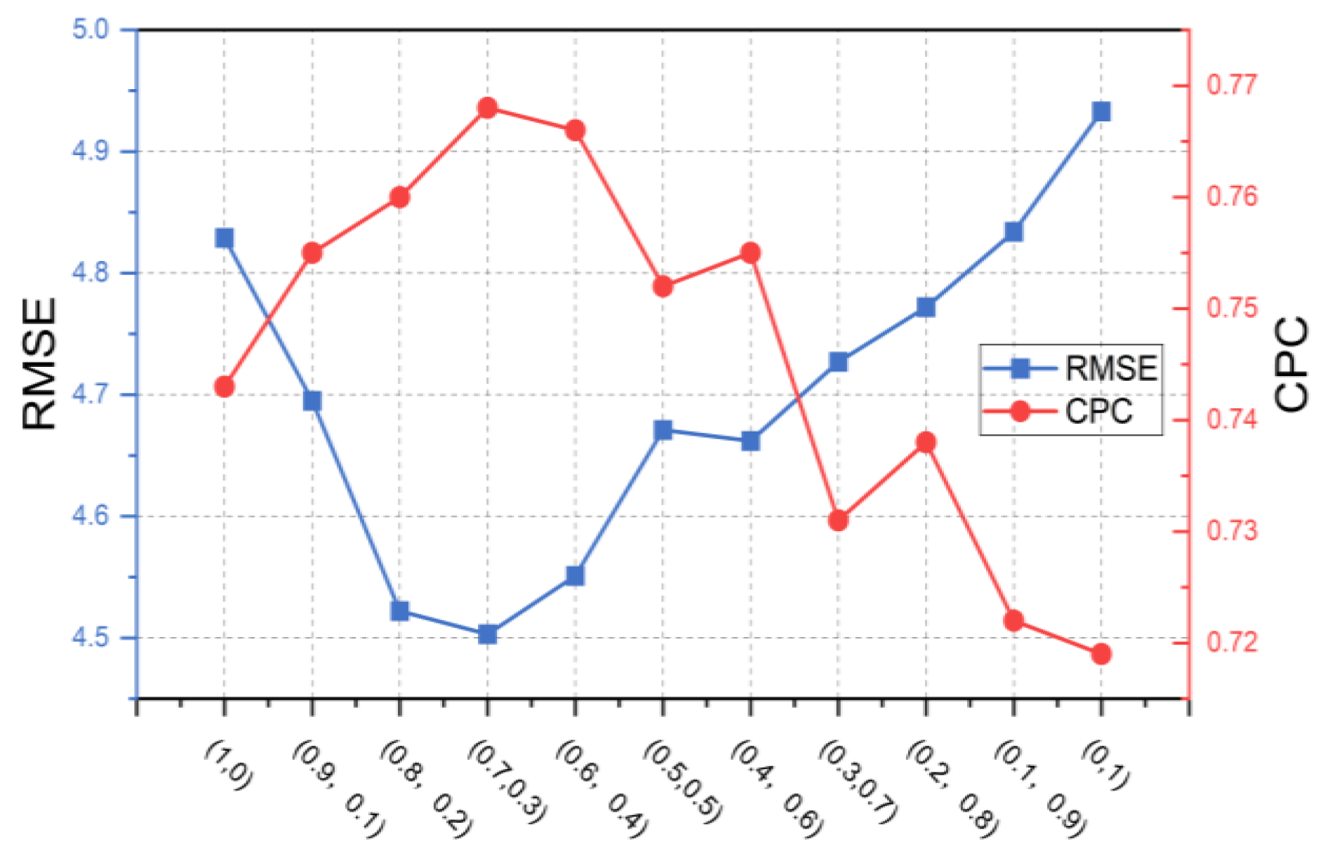
4.2. Decoder Using Multitask Learning for GLGAT Training
4.3. Flow Inference Using XGBoost for OD Flow Inference
5. Experiment Description
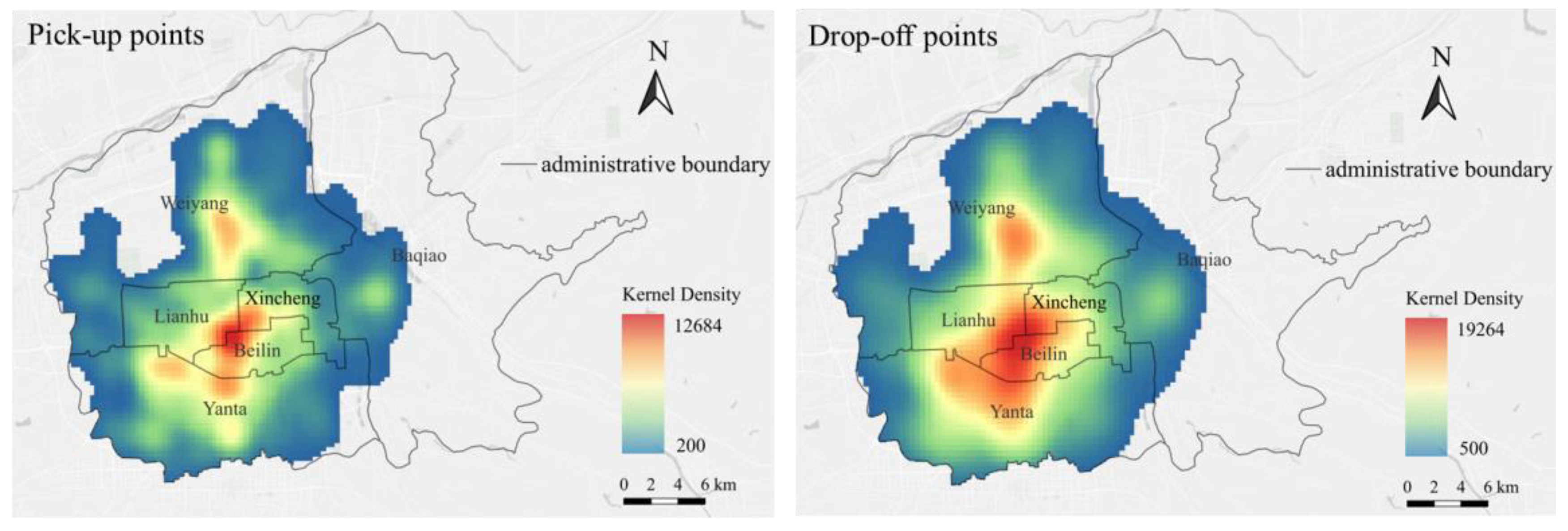
5.1. Data Description and Preprocessing
| Algorithm 1. Origin and Destination Extraction Algorithm |
| Input: T: Taxi trajectory dataset, where each ti represents a trip with a sequence of ordered points. Output: O: Set of origin points from T D: Set of destination points from T Procedure: Initialize: O = [], D = [] For each trip ti in T: Sorting: Sort data by “Vehicle Num” and then by “Time”. Shift: Use Shift() to move “Status” down by one row, storing the result in “Status_next”. Compute: Calculate Status Change = Status—Status_next: If Status Change == 1: Add to O ElseIf Status Change == −1: Add to D Return O, D |
5.2. Baseline Models
- Gravity Model [10]. This is a classical model that proposes that OD flow between two zones is directly proportional to population and inversely proportional to distance.
- RF. This is a decision tree ensemble learning approach to circumvent overfitting and enhance performance. In this study, urban features and distance are directly concatenated as input to infer OD flows.
- GBRT. This is an iterative decision tree generation algorithm consisting of multiple decision trees as weak learners.
- XGBoost. This is a gradient boosting tree model that can be considered state of the art in many classification and regression tasks.
- Deep Gravity [14]. This is an enhanced version of the gravity model that takes more factors into account when modeling by using an FCNN.
- GCN [16]. This uses GCNs to embed information about urban features in geographically neighboring regions and uses a bilinear function to infer OD flows.
- GCN-RF [18]. This is similar to the abovementioned GCN model; however, the OD flows are inferred by using the RF.
- GMEL [17]. This uses two separate GATs to learn and generate embeddings for origin and destination, respectively. The GBRT is used to infer OD flows.
5.3. Experiment Setting
5.4. Evaluation Metrics
6. Results and Discussion
6.1. Performance Comparison with Baselines (RQ 1)
6.2. Performance Comparison with Model Variants (RQ 2)
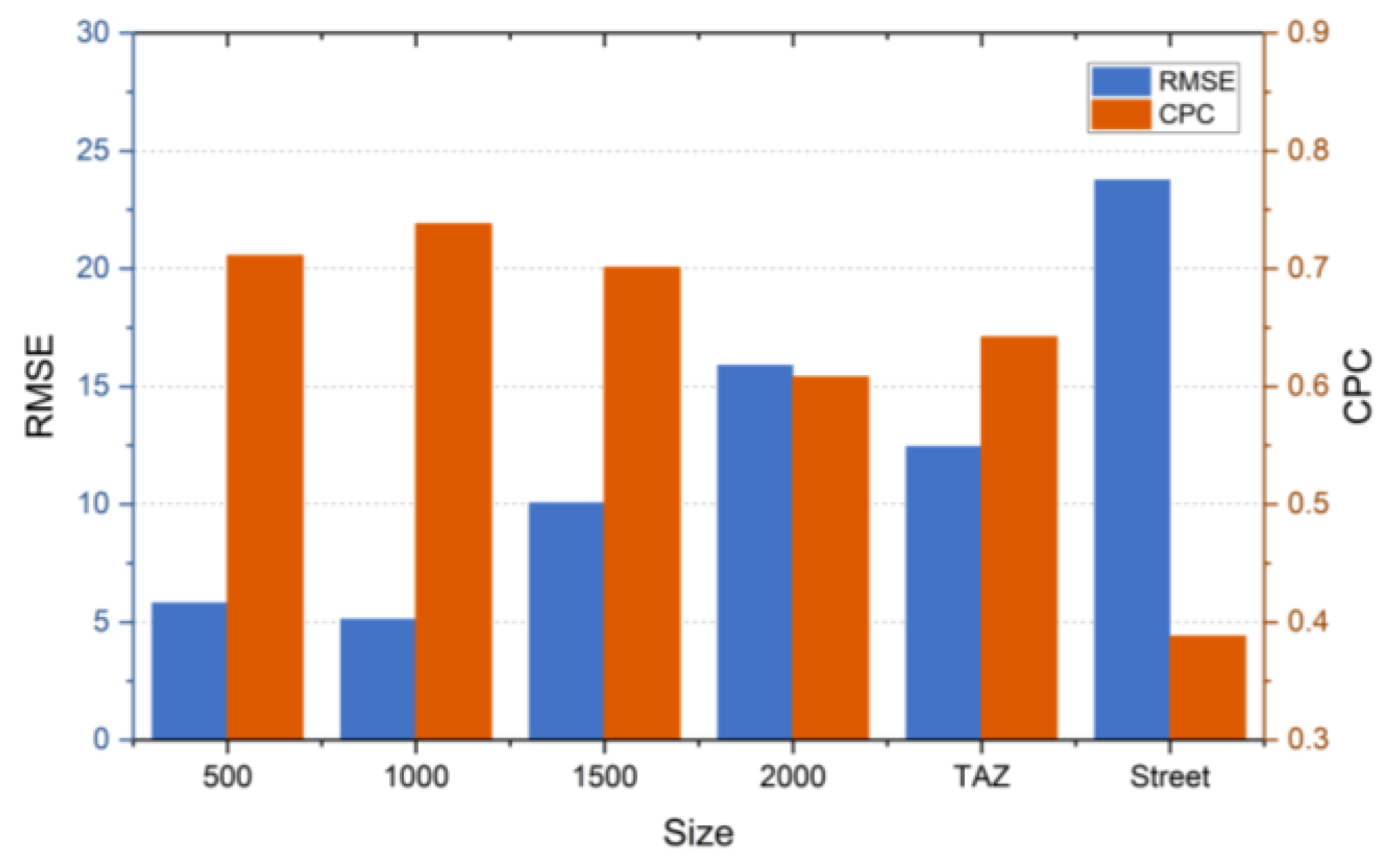
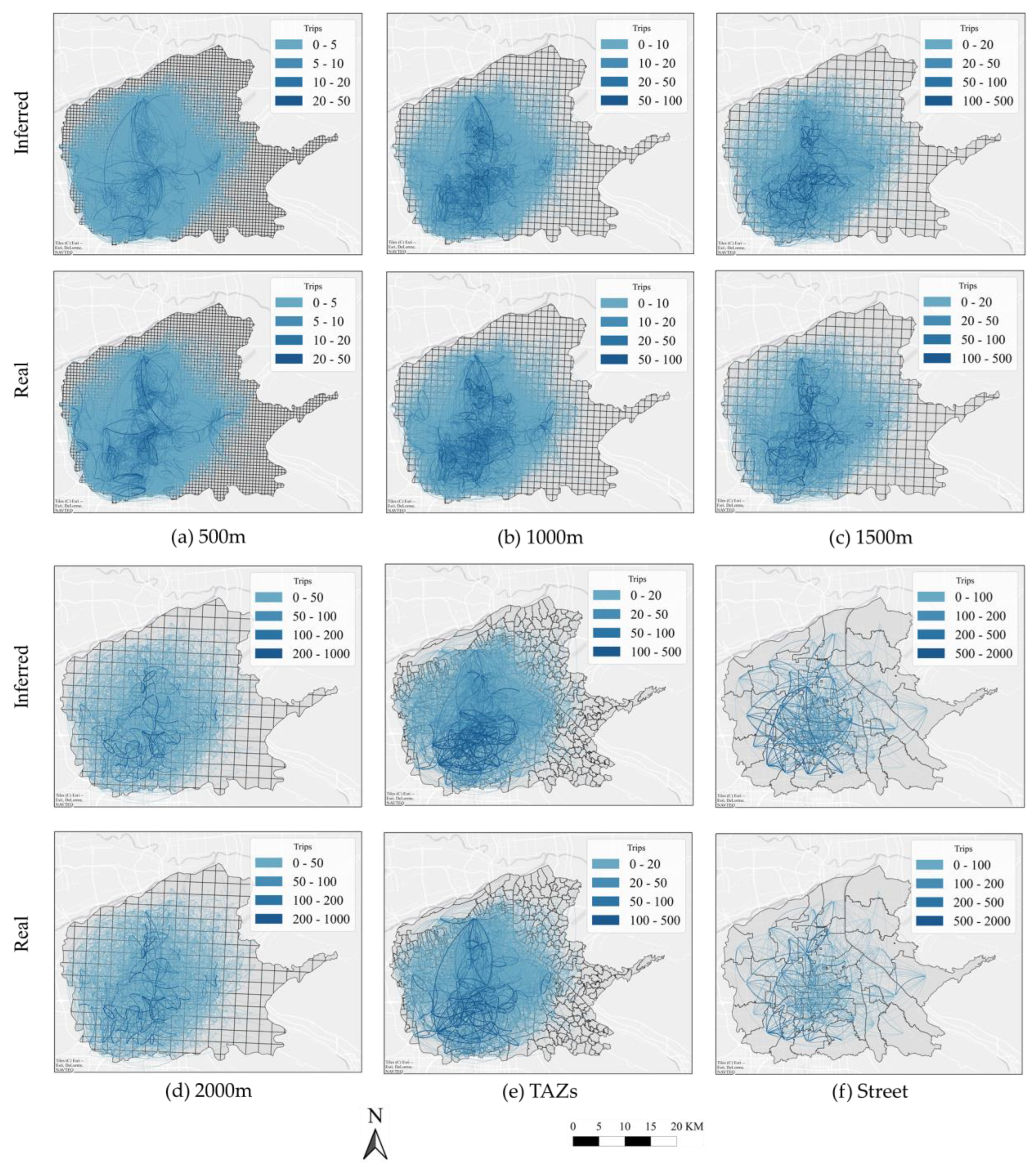
6.3. Performance Comparison with Multi-Scale Units of Analysis (RQ 3)
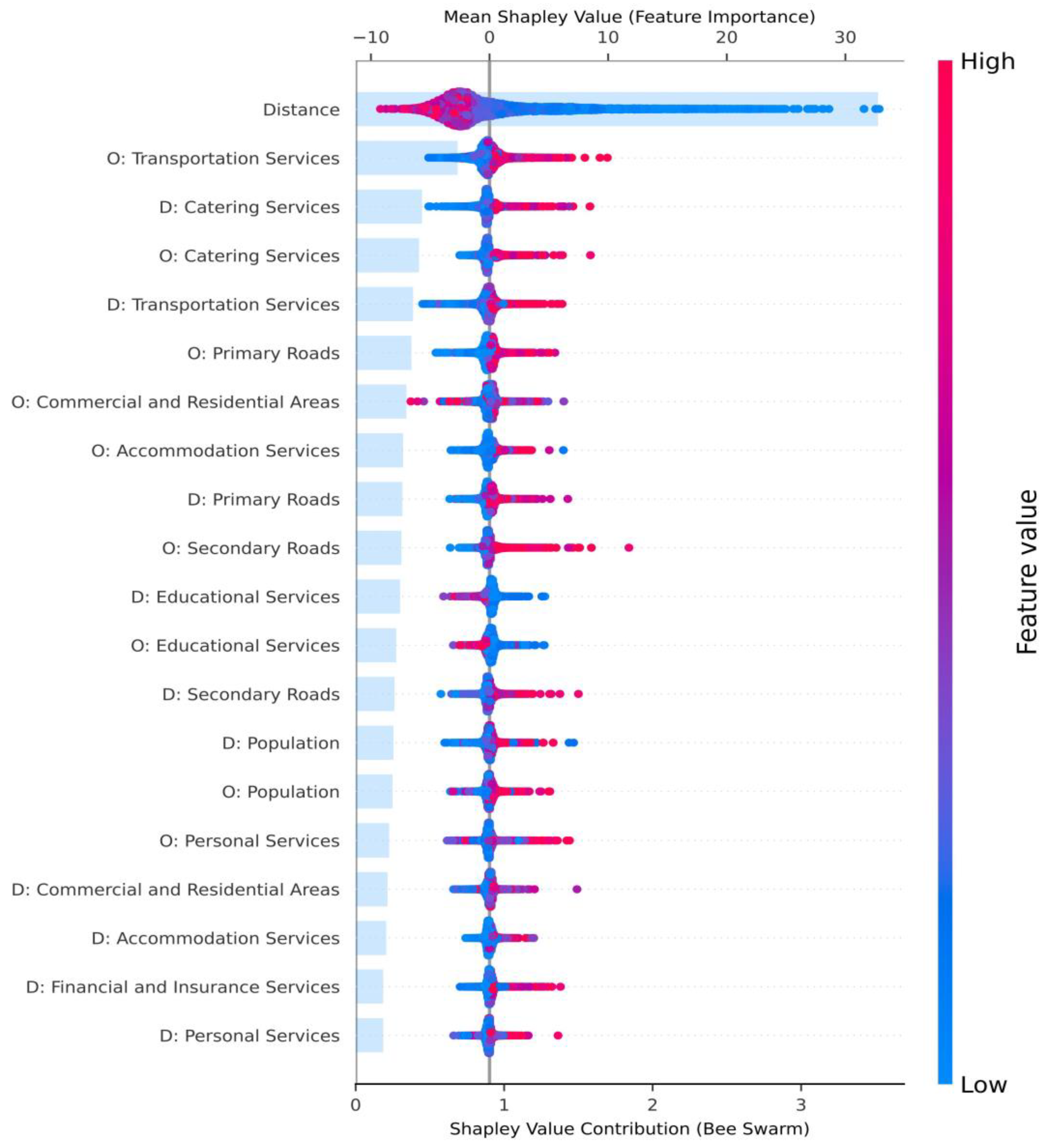
6.4. An Interpretation of the Impact of Urban Features (RQ 4)
6.5. The Application of the GLGAT-XG Model (RQ 5)
7. Conclusions
Author Contributions
Funding
Data Availability Statement
Acknowledgments
Conflicts of Interest
References
- Zhao, Y.; Cheng, S.; Gao, S.; Wang, P.; Lu, F. Predicting origin-destination flows by considering heterogeneous mobility patterns. Sustain. Cities Soc. 2025, 118, 106015. [Google Scholar] [CrossRef]
- Hu, T.; Wang, S.; She, B.; Zhang, M.; Huang, X.; Cui, Y.; Khuri, J.; Hu, Y.; Fu, X.; Wang, X.; et al. Human Mobility Data in the COVID-19 Pandemic: Characteristics, Applications, and Challenges. Int. J. Digit. Earth 2021, 14, 1126–1147. [Google Scholar] [CrossRef]
- Casali, Y.; Aydin, N.Y.; Comes, T. Machine Learning for Spatial Analyses in Urban Areas: A Scoping Review. Sustain. Cities Soc. 2022, 85, 104050. [Google Scholar] [CrossRef]
- Fadlullah, Z.M.; Tang, F.; Mao, B.; Kato, N.; Akashi, O.; Inoue, T.; Mizutani, K. State-of-the-Art Deep Learning: Evolving Machine Intelligence toward Tomorrow’s Intelligent Network Traffic Control Systems. IEEE Commun. Surv. Tutor. 2017, 19, 2432–2455. [Google Scholar] [CrossRef]
- Bassolas, A.; Barbosa-Filho, H.; Dickinson, B.; Dotiwalla, X.; Eastham, P.; Gallotti, R.; Ghoshal, G.; Gipson, B.; Hazarie, S.A.; Kautz, H.; et al. Hierarchical Organization of Urban Mobility and Its Connection with City Livability. Nat. Commun. 2019, 10, 4817. [Google Scholar] [CrossRef]
- Wang, J.; Song, J.; Zhao, C.; Ban, X.J. Distributionally robust origin–destination demand estimation. Transp. Res. Part C Emerg. Technol. 2024, 165, 104716. [Google Scholar] [CrossRef]
- Kamel Boulos, M.N.; Kwan, M.-P.; El Emam, K.; Chung, A.L.-L.; Gao, S.; Richardson, D.B. Reconciling Public Health Common Good and Individual Privacy: New Methods and Issues in Geoprivacy. Int. J. Health Geogr. 2022, 21, 1. [Google Scholar] [CrossRef]
- Savage, N. Synthetic Data Could Be Better than Real Data. Nature 2023. [Google Scholar] [CrossRef]
- Liu, K. Approaches for Human Mobility Data Generation: Research Progress and Trends. J. Geo-Inf. Sci. 2024, 26, 1–12. [Google Scholar] [CrossRef]
- Zipf, G.K. The P 1 p 2 D Hypothesis: On the Intercity Movement of Persons. Am. Sociol. Rev. 1946, 11, 677. [Google Scholar] [CrossRef]
- Simini, F.; González, M.C.; Maritan, A.; Barabási, A.-L. A Universal Model for Mobility and Migration Patterns. Nature 2012, 484, 96–100. [Google Scholar] [CrossRef] [PubMed]
- Stouffer, S.A. Intervening Opportunities: A Theory Relating Mobility and Distance. Am. Sociol. Rev. 1940, 5, 845. [Google Scholar] [CrossRef]
- Pourebrahim, N.; Sultana, S.; Niakanlahiji, A.; Thill, J.-C. Trip Distribution Modeling with Twitter Data. Comput. Environ. Urban Syst. 2019, 77, 101354. [Google Scholar] [CrossRef]
- Simini, F.; Barlacchi, G.; Luca, M.; Pappalardo, L. A Deep Gravity Model for Mobility Flows Generation. Nat. Commun. 2021, 12, 6576. [Google Scholar] [CrossRef]
- Robinson, C.; Dilkina, B. A Machine Learning Approach to Modeling Human Migration. In Proceedings of the 1st ACM SIGCAS Conference on Computing and Sustainable Societies, Menlo Park, CA, USA, 20–21 June 2018; pp. 1–8. [Google Scholar] [CrossRef]
- Yao, X.; Gao, Y.; Zhu, D.; Manley, E.; Wang, J.; Liu, Y. Spatial Origin-Destination Flow Imputation Using Graph Convolutional Networks. IEEE Trans. Intell. Transp. Syst. 2021, 22, 7474–7484. [Google Scholar] [CrossRef]
- Liu, Z.; Miranda, F.; Xiong, W.; Yang, J.; Wang, Q.; Silva, C. Learning Geo-Contextual Embeddings for Commuting Flow Prediction. Proc. AAAI Conf. Artif. Intell. 2020, 34, 808–816. [Google Scholar] [CrossRef]
- Yin, G.; Huang, Z.; Bao, Y.; Wang, H.; Li, L.; Ma, X.; Zhang, Y. CONVGCN-RF: A Hybrid Learning Model for Commuting Flow Prediction Considering Geographical Semantics and Neighborhood Effects. GeoInformatica 2022, 27, 137–157. [Google Scholar] [CrossRef]
- Shi, Q.; Zhuo, L.; Tao, H.; Yang, J. A Fusion Model of Temporal Graph Attention Network and Machine Learning for Inferring Commuting Flow from Human Activity Intensity Dynamics. Int. J. Appl. Earth Obs. Geoinf. 2024, 126, 103610. [Google Scholar] [CrossRef]
- Klemmer, K.; Safir, N.S.; Neill, D.B. Positional Encoder Graph Neural Networks for Geographic Data. In Proceedings of the International Conference on Artificial Intelligence and Statistics, Virtual Conference, 25–27 April 2023; pp. 1379–1389. [Google Scholar] [CrossRef]
- Wu, Q.; Zhao, W.; Li, Z.; Wipf, D.; Yan, J. Nodeformer: A Scalable Graph Structure Learning Transformer for Node Classification. In Proceedings of the 36th Conference on Neural Information Processing Systems (NeurIPS), New Orleans, LA, USA, 10–16 December 2022. [Google Scholar] [CrossRef]
- Yan, X.-Y.; Zhao, C.; Fan, Y.; Di, Z.; Wang, W.-X. Universal Predictability of Mobility Patterns in Cities. J. R. Soc. Interface 2014, 11, 20140834. [Google Scholar] [CrossRef]
- Pei, T.; Liu, Y.X.; Guo, S.H.; Shu, H.; Du, Y.; Ma, T.; Zhou, C. Principle of Big Geodata Mining. Acta Geogr. Sin. 2019, 74, 586–598. [Google Scholar] [CrossRef]
- Lv, C.; Qi, M.; Li, X.; Yang, Z.; Ma, H. Sgformer: Semantic Graph Transformer for Point Cloud-Based 3D Scene Graph Generation. Proc. AAAI Conf. Artif. Intell. 2024, 38, 4035–4043. [Google Scholar] [CrossRef]
- Liu, E.; Yan, X. New Parameter-Free Mobility Model: Opportunity Priority Selection Model. Phys. A 2019, 526, 121023. [Google Scholar] [CrossRef]
- Tobler, W.R. A Computer Movie Simulating Urban Growth in the Detroit Region. Econ. Geogr. 1970, 46 (Suppl. 1), 234. [Google Scholar] [CrossRef]
- Xing, X.; Huang, Z.; Cheng, X.; Zhu, D.; Kang, C.; Zhang, F.; Liu, Y. Mapping human activity volumes through remote sensing imagery. IEEE J. Sel. Top. Appl. Earth Obs. Remote Sens. 2020, 13, 5652–5668. [Google Scholar] [CrossRef]
- Kipf, T.N.; Welling, M. Semi-Supervised Classification with Graph Convolutional Networks. In Proceedings of the International Conference on Learning Representations, Toulon, France, 24–26 April 2017. [Google Scholar] [CrossRef]
- Pan, Z.; Liang, Y.; Wang, W.; Yu, Y.; Zheng, Y.; Zhang, J. Urban Traffic Prediction from Spatio-Temporal Data Using Deep Meta Learning. In Proceedings of the 25th ACM SIGKDD International Conference on Knowledge Discovery & Data Mining, Anchorage, AK, USA, 4–8 August 2019. [Google Scholar] [CrossRef]
- Wang, Y.; Yin, H.; Chen, H.; Wo, T.; Xu, J.; Zheng, K. Origin-Destination Matrix Prediction via Graph Convolution. In Proceedings of the 25th ACM SIGKDD International Conference on Knowledge Discovery & Data Mining, Anchorage, AK, USA, 4–8 August 2019. [Google Scholar] [CrossRef]
- Cheng, Z.; Trépanier, M.; Sun, L. Real-Time Forecasting of Metro Origin-Destination Matrices with High-Order Weighted Dynamic Mode Decomposition. Transp. Sci. 2022, 56, 904–918. [Google Scholar] [CrossRef]
- Zhang, Y.; Sun, K.; Wen, D.; Chen, D.; Lv, H.; Zhang, Q. Deep Learning for Metro Short-Term Origin-Destination Passenger Flow Forecasting Considering Section Capacity Utilization Ratio. IEEE Trans. Intell. Transp. Syst. 2023, 24, 7943–7960. [Google Scholar] [CrossRef]
- Lv, S.; Wang, K.; Yang, H.; Wang, P. An Origin–Destination Passenger Flow Prediction System Based on Convolutional Neural Network and Passenger Source-Based Attention Mechanism. Expert Syst. Appl. 2024, 238, 121989. [Google Scholar] [CrossRef]
- Li, Q.; Han, Z.; Wu, X.-M. Deeper Insights into Graph Convolutional Networks for Semi-Supervised Learning. In Proceedings of the AAAI Conference on Artificial Intelligence, New Orleans, LA, USA, 2–7 February 2018. [Google Scholar] [CrossRef]
- Alon, U.; Yahav, E. On the Bottleneck of Graph Neural Networks and Its Practical Implications. In Proceedings of the International Conference on Learning Representations, Virtual Conference, 3–7 May 2021. [Google Scholar] [CrossRef]
- Nejadshamsi, S.; Bentahar, J.; Eicker, U.; Wang, C.; Jamshidi, F. A Geographic-Semantic Context-Aware Urban Commuting Flow Prediction Model Using Graph Neural Network. Expert Syst. Appl. 2025, 261, 125534. [Google Scholar] [CrossRef]
- Zhang, B.; Fan, C.; Liu, S.; Huang, K.; Zhao, X.; Huang, J.; Liu, Z. The Expressive Power of Graph Neural Networks: A Survey. IEEE Trans. Knowl. Data Eng. 2025, 37, 1455–1474. [Google Scholar] [CrossRef]
- Wang, L.; Geng, X.; Ma, X.; Liu, F.; Yang, Q. Cross-City Transfer Learning for Deep Spatio-Temporal Prediction. In Proceedings of the 28th International Joint Conference on Artificial Intelligence, Macao, China, 10–16 August 2019; pp. 1893–1899. [Google Scholar] [CrossRef]
- Guo, J.; Bai, S.; Li, X.; Xian, K.; Liu, E.; Ding, W.; Ma, X. A Universal Geography Neural Network for Mobility Flow Prediction in Planning Scenarios. Comput.-Aided Civ. Infrastruct. Eng. 2025; in press. [Google Scholar] [CrossRef]
- Wu, Z.H.; Jain, P.; Wright, M.A.; Mirhoseini, A.; Gonzalez, J.E.; Stoica, I. Representing Long-Range Context for Graph Neural Networks with Global Attention. In Proceedings of the 35th Conference on Neural Information Processing Systems (NeurIPS), Virtual Conference, 6–14 December 2021. [Google Scholar] [CrossRef]
- Cai, M.; Pang, Y.; Sekimoto, Y. Spatial Attention Based Grid Representation Learning for Predicting Origin–Destination Flow. In Proceedings of the 2022 IEEE International Conference on Big Data (Big Data), Osaka, Japan, 13–16 December 2022; pp. 485–494. [Google Scholar] [CrossRef]
- Rong, C.; Ding, J.; Li, Y. An Interdisciplinary Survey on Origin-Destination Flows Modeling: Theory and Techniques. ACM Comput. Surv. 2024, 57, 1–49. [Google Scholar] [CrossRef]
- Chen, Y.; Xu, C.; Ge, Y.; Zhang, X.; Zhou, Y. A 100-M Gridded Population Dataset of China’s Seventh Census Using Ensemble Learning and Geospatial Big Data. Earth Syst. Sci. Data, 2024; Submitted. [Google Scholar] [CrossRef]


| Type | Name | Technique | Main Module | Year | Data | Spatial Scale |
|---|---|---|---|---|---|---|
| Traditional methods | Gravity [10] | Mathematical Model | - | 1946 | Population, Distance | TAZ |
| Radiation [11] | Mathematical Model | - | 2012 | Population | county | |
| PWO [22] | Mathematical Model | - | 2014 | Opportunity, Population | county | |
| OPS [25] | Mathematical Model | - | 2019 | Opportunity, Population | county | |
| ML-based methods | RF [15] | Tree-Based Model | RF | 2018 | Socioeconomic | census tract |
| ANN [13] | Neural Network | ANNs | 2019 | Socioeconomic | census tract | |
| Deep Gravity [14] | Neural Network | FFNN | 2021 | Socioeconomic, Distance | county | |
| GNN-based methods | GMEL [17] | Deep Learning | GAT + GBRT | 2020 | Socioeconomic, Distance | census tract |
| SI-GCN [16] | Deep Learning | GCN | 2021 | Position, Number Of Passengers | 1 km grid | |
| ConvGCN-RF [18] | Deep Learning | GAT + RF | 2023 | Population, Land use | 500 m grid | |
| TGAT-ML [19] | Deep Learning | TGAT + GBRT | 2024 | Heatmap, Distance | 1 km grid |
| Datasets | Features | Contents |
|---|---|---|
| POIs | 13 | Number of different types of POI facilities in 2020 |
| Roads | 22 | The road length varies according to the road grade in 2020 |
| Distance | 1 | Linear distance between zone centers of mass |
| Population | 1 | Population distribution in 2020 |
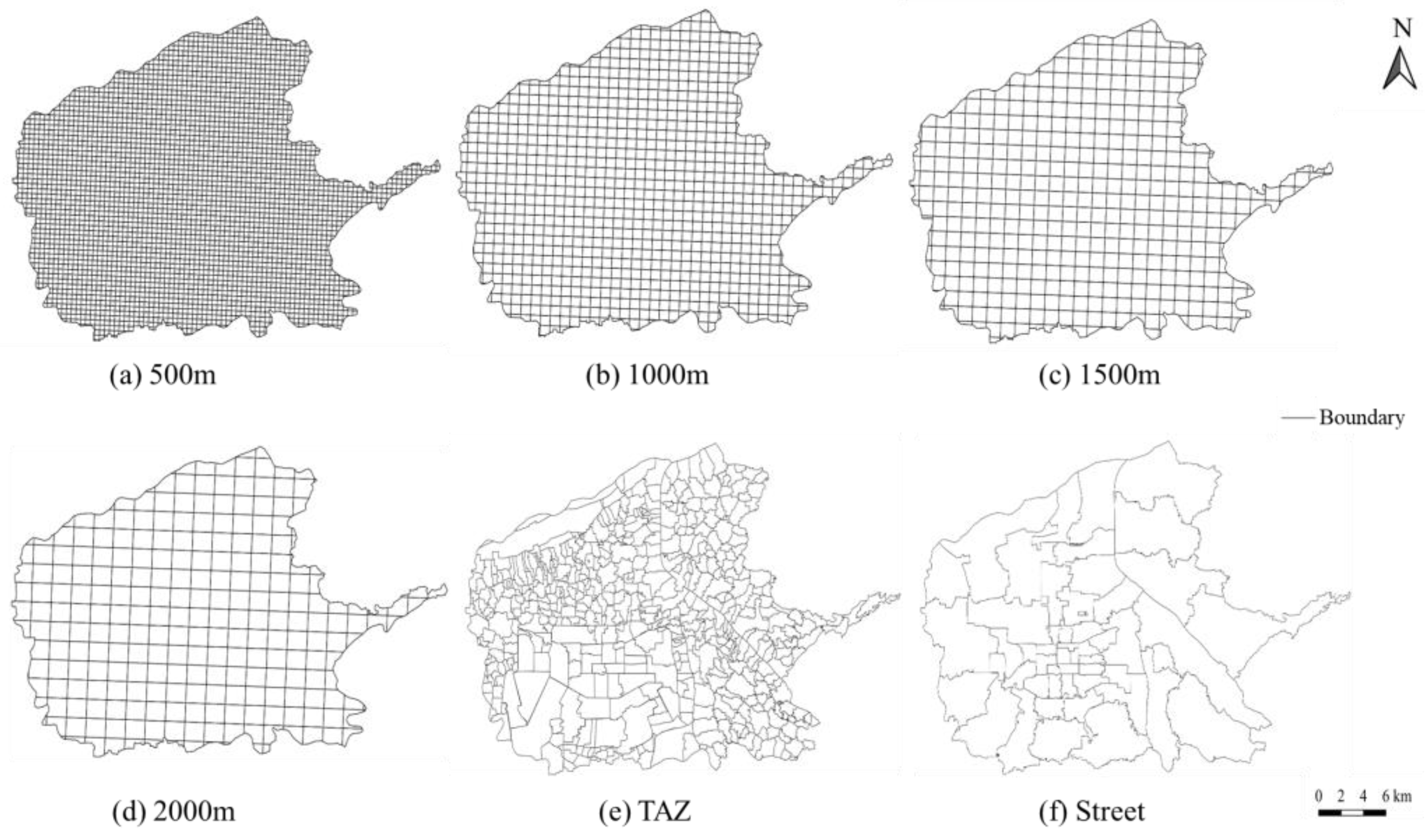
| Size (m) | Number | Average Area (km2) | Size (m) | Number | Average Area (km2) |
|---|---|---|---|---|---|
| 500 × 500 | 3558 | 0.24 | 2000 × 2000 | 254 | 3.33 |
| 1000 × 1000 | 938 | 0.90 | Street | 51 | 16.61 |
| 1500 × 1500 | 441 | 1.92 | TAZs | 503 | 1.68 |
| Model | NYC | LA | Sea | ||||||
|---|---|---|---|---|---|---|---|---|---|
| RMSE | MAE | CPC | RMSE | MAE | CPC | RMSE | MAE | CPC | |
| Gravity | 9.496 | 4.223 | 0.482 | 16.559 | 6.992 | 0.311 | 26.168 | 12.752 | 0.268 |
| RF | 6.493 | 3.561 | 0.565 | 12.134 | 5.025 | 0.338 | 19.752 | 10.322 | 0.301 |
| GBRT | 5.991 | 2.833 | 0.599 | 11.768 | 3.742 | 0.416 | 19.697 | 10.870 | 0.328 |
| XGBoost | 5.748 | 2.556 | 0.608 | 10.932 | 3.963 | 0.492 | 17.815 | 9.053 | 0.311 |
| Deep Gravity | 6.814 | 2.732 | 0.615 | 11.367 | 3.982 | 0.441 | 16.910 | 9.263 | 0.309 |
| GCN | 5.962 | 2.130 | 0.651 | 11.192 | 3.523 | 0.521 | 13.972 | 8.160 | 0.483 |
| GCN-RF | 5.301 | 1.992 | 0.701 | 10.673 | 2.913 | 0.575 | 12.671 | 7.260 | 0.483 |
| GMEL | 4.887 | 1.747 | 0.741 | 8.819 | 2.762 | 0.624 | 11.972 | 5.060 | 0.542 |
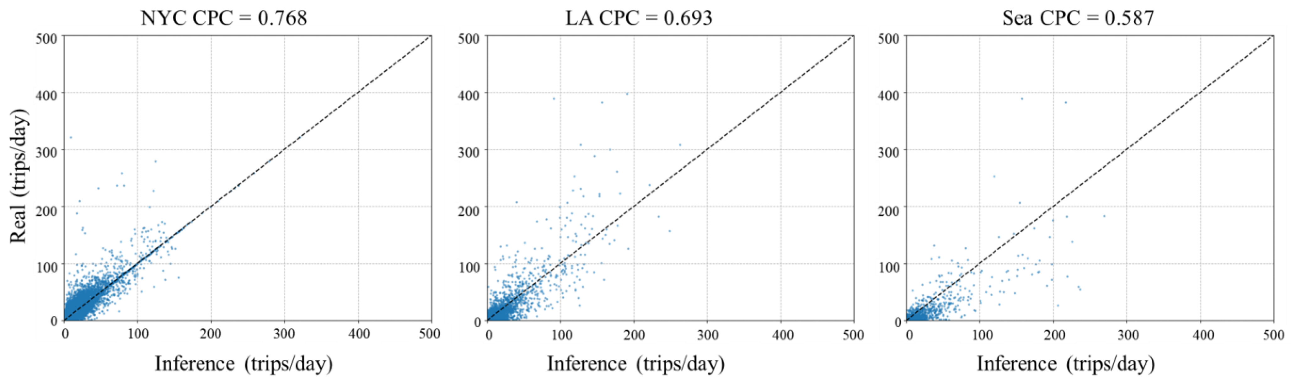
| GLGAT-XG | 4.503 | 1.685 | 0.768 | 7.522 | 2.718 | 0.693 | 10.247 | 4.640 | 0.587 |
| Model | MAE | RMSE | CPC |
|---|---|---|---|
| GLGAT-RF | 4.880 | 1.892 | 0.712 |
| GLGAT-GBRT | 4.602 | 1.733 | 0.744 |
| GCN-XGBoost | 5.261 | 2.033 | 0.703 |
| GAT-XGBoost | 4.829 | 1.730 | 0.743 |
| GLGAT-XGBoost | 4.503 | 1.685 | 0.768 |
Disclaimer/Publisher’s Note: The statements, opinions and data contained in all publications are solely those of the individual author(s) and contributor(s) and not of MDPI and/or the editor(s). MDPI and/or the editor(s) disclaim responsibility for any injury to people or property resulting from any ideas, methods, instructions or products referred to in the content. |
© 2025 by the authors. Published by MDPI on behalf of the International Society for Photogrammetry and Remote Sensing. Licensee MDPI, Basel, Switzerland. This article is an open access article distributed under the terms and conditions of the Creative Commons Attribution (CC BY) license (https://creativecommons.org/licenses/by/4.0/).
Share and Cite
Shan, Z.; Yang, F.; Shi, X.; Cui, Y. Hybrid Learning Model of Global–Local Graph Attention Network and XGBoost for Inferring Origin–Destination Flows. ISPRS Int. J. Geo-Inf. 2025, 14, 182. https://doi.org/10.3390/ijgi14050182
Shan Z, Yang F, Shi X, Cui Y. Hybrid Learning Model of Global–Local Graph Attention Network and XGBoost for Inferring Origin–Destination Flows. ISPRS International Journal of Geo-Information. 2025; 14(5):182. https://doi.org/10.3390/ijgi14050182
Chicago/Turabian StyleShan, Zhenyu, Fei Yang, Xingzi Shi, and Yaping Cui. 2025. "Hybrid Learning Model of Global–Local Graph Attention Network and XGBoost for Inferring Origin–Destination Flows" ISPRS International Journal of Geo-Information 14, no. 5: 182. https://doi.org/10.3390/ijgi14050182
APA StyleShan, Z., Yang, F., Shi, X., & Cui, Y. (2025). Hybrid Learning Model of Global–Local Graph Attention Network and XGBoost for Inferring Origin–Destination Flows. ISPRS International Journal of Geo-Information, 14(5), 182. https://doi.org/10.3390/ijgi14050182