Article

End-to-End Vector Simplification for Building Contours via a Sequence Generation Model

1
Institute of Geospatial Information, Information Engineering University, Zhengzhou 450052, China
2
State Key Laboratory of Complex Electromagnetic Environment Effects on Electronics and Information System, Luoyang 471000, China
3
College of Geography and Environmental Science, Henan University, Kaifeng 475000, China
*
Author to whom correspondence should be addressed.
ISPRS Int. J. Geo-Inf. 2025, 14(3), 124; https://doi.org/10.3390/ijgi14030124
Submission received: 2 January 2025 / Revised: 6 March 2025 / Accepted: 8 March 2025 / Published: 9 March 2025

Abstract

:
Simplifying building contours involves reducing data volume while preserving the continuity, accuracy, and essential characteristics of building shapes. This presents significant challenges for sequence representation and generation. Traditional methods often rely on complex rule design, feature engineering, and iterative optimization. To overcome these limitations, this study proposes a Transformer-based Polygon Simplification Model (TPSM) for the end-to-end vector simplification of building contours. TPSM processes ordered vertex coordinate sequences of building contours, leveraging the inherent sequence modeling capabilities of the Transformer architecture to directly generate simplified coordinate sequences. To enhance spatial understanding, positional encoding is embedded within the multihead self-attention mechanism, allowing the TPSM to effectively capture relative vertex positions. Additionally, a self-supervised reconstruction mechanism is introduced, where random perturbations are applied to input sequences, and the model learns to reconstruct the original contours. This mechanism enables TPSM to better understand underlying geometric relationships and implicit simplification rules. Experiments were conducted using a 1:10,000 building dataset from Shenzhen, China, targeting a simplification scale of 1:25,000. The results demonstrate that TPSM outperforms five established simplification algorithms in controlling changes to building area, orientation, and shape fidelity, achieving an average intersection over union (IoU) of 0.901 and a complexity-aware IoU (C-IoU) of 0.735.

1. Introduction

Cartographic generalization aims to represent geometric elements on maps concisely and clearly while reducing the map scale. This is a crucial stage in cartographic production [1,2]. Vector contour simplification is a key technique for generalization. As significant features on maps, buildings play a vital role in representing human activity and analyzing urban planning. Accurate and concise building outlines are essential for depicting these aspects at various scales. However, building outlines extracted from remote sensing imagery and raster maps often exhibit imperfections, such as jagged boundaries, redundant points, and blurred corners, as shown in Figure 1. These require regularization and simplification to meet cartographic standards [3].
Building contour simplification aims to retain key geometric characteristics, including shape, area, perimeter, and orientation, while expressing the building features in a succinct manner suitable for the chosen scale and thematic focus [4]. Current research on building contour simplification primarily focuses on the efficient removal of redundant points based on local features, preserving orthogonality after simplification, and balancing the tradeoff between simplification and preservation of key features. However, many existing methods require complex rule design, data transformations for feature extraction, and meticulous hyperparameter tuning, which limit their applicability and generalizability. Furthermore, these methods often struggle to capture long-range dependencies within the contour sequence, leading to suboptimal simplification results for complex building shapes [5]. A significant limitation of many recent deep learning approaches is their reliance on raster data [6,7]. These methods necessitate the rasterization of vector building outlines, which inevitably leads to a loss of precise geometric information. The subsequent vectorization of the simplified raster representation introduces additional processing steps and the potential for further errors and inaccuracies. Moreover, some of these methods impose fixed input and output lengths, requiring interpolation to standardize the number of points, thus limiting the model’s flexibility and hindering its ability to handle buildings of varying complexity. Many deep learning approaches also face challenges in terms of scalability, struggling to efficiently process very large datasets or extremely complex building outlines. Additionally, the performance of these models is often heavily reliant on the availability of large, high-quality labeled datasets, which can be a significant bottleneck in practical applications, especially for specialized tasks like building simplification at specific scales. However, it is crucial to acknowledge that, while end-to-end vector generalization methods offer significant advantages, they also present potential risks of introducing topological errors, such as overlaps and gaps, during the simplification process. Therefore, developing an end-to-end method capable of directly processing vector sequences and automatically performing building simplification and regularization is crucial for enhancing cartographic efficiency and improving algorithmic versatility, but future research needs to carefully address the issue of maintaining topological consistency to ensure the reliability and usability of the simplified building outlines.
The existing building simplification methods can be broadly categorized into four groups: rule-based methods, optimization-based methods, machine-learning-based methods, and deep-learning-based methods. Rule-based methods rely on predefined rules based on the building geometry. Early research concentrated on line simplification algorithms, such as the Douglas–Peucker [8], Li–Openshaw [9], and Visvalingam–Whyatt [10] algorithms, which operate based on the principles of perpendicular distance, minimum visible object, and effective area, respectively. Rule-based building simplification methods typically involve template matching [11,12,13] and local structure simplification [14,15]. Template matching substitutes the original building with predefined templates, whereas local structure simplification streamlines the building based on local features such as right angles and concavities. Although conceptually straightforward, rule-based methods suffer from limitations owing to their reliance on expert-defined rules, which struggle to accommodate the diverse complexities of building shapes.
Optimization-based methods formulate building simplification as an optimization problem. For instance, least-squares adjustment can be utilized by incorporating operations such as offsetting, squeezing, and corner manipulation as fundamental units to minimize errors and achieve simplification [16]. Additionally, a combination of the Douglas–Peucker algorithm and least squares was proposed as a recursive simplification method [17]. Haunert and Wolff ensured topological safety by selecting subsequences of the original building edges [18]. Although optimization-based methods can preserve the overall building shape to a certain extent, they are computationally intensive and sensitive to parameter settings.
With the advent of machine learning, researchers have increasingly applied techniques to simplify buildings. Simplification can be achieved by using support vector machines for line feature simplification [19], classifying and simplifying building models based on convolutional neural networks [20], and learning cartographic rules using backpropagation neural networks. This involves utilizing knowledge of raster features [21] and existing simplification methods [4]. Machine learning methods can automatically learn simplification rules, exhibiting strong adaptability; however, they require extensive training data and often lack model interpretability.
Recently, deep learning methods, particularly convolutional neural networks (CNNs) and generative adversarial networks (GANs), have shown promise in simplifying buildings. Sester et al. [22] and Feng et al. [23] utilized U-Net models, Courtial et al. employed GANs and U-Nets for mountain road generalization [24,25], Du et al. used a Pix2Pix model for line simplification [26], and Yu and Chen used an encoder–decoder network to generate multilevel simplified lines [27]. These methods demonstrate the potential of deep learning for simplification. However, their reliance on raster data necessitates the rasterization of vector data, which inevitably leads to geometric information loss. The simplified results then require vectorization, the introduction of additional processing steps, and potential errors. Furthermore, some methods impose fixed input and output lengths, requiring interpolation to standardize the number of points and thus limiting the models’ flexibility and hindering their ability to handle buildings of varying complexity.
To overcome the limitations of the existing methods and apply deep learning directly to vector data, this study proposes the Transformer-based Polygon Simplification Model (TPSM). This method uses the vector coordinate sequence of a building outline as the input and leverages the powerful sequence modeling capabilities of the Transformer network to directly generate a simplified vector coordinate sequence.
The primary contributions of this paper are as follows:
  • End-to-end vector simplification: TPSM is introduced, which is capable of directly handling vector data and generating simplified vector coordinate sequences, thereby enabling end-to-end learning for building simplification.
  • Enhanced shape feature extraction: The multihead attention mechanism is analyzed and improved upon by integrating position encoding directly into the attention mechanism. This allows the TPSM to more effectively capture the shape features inherent in the vector sequence coordinates.
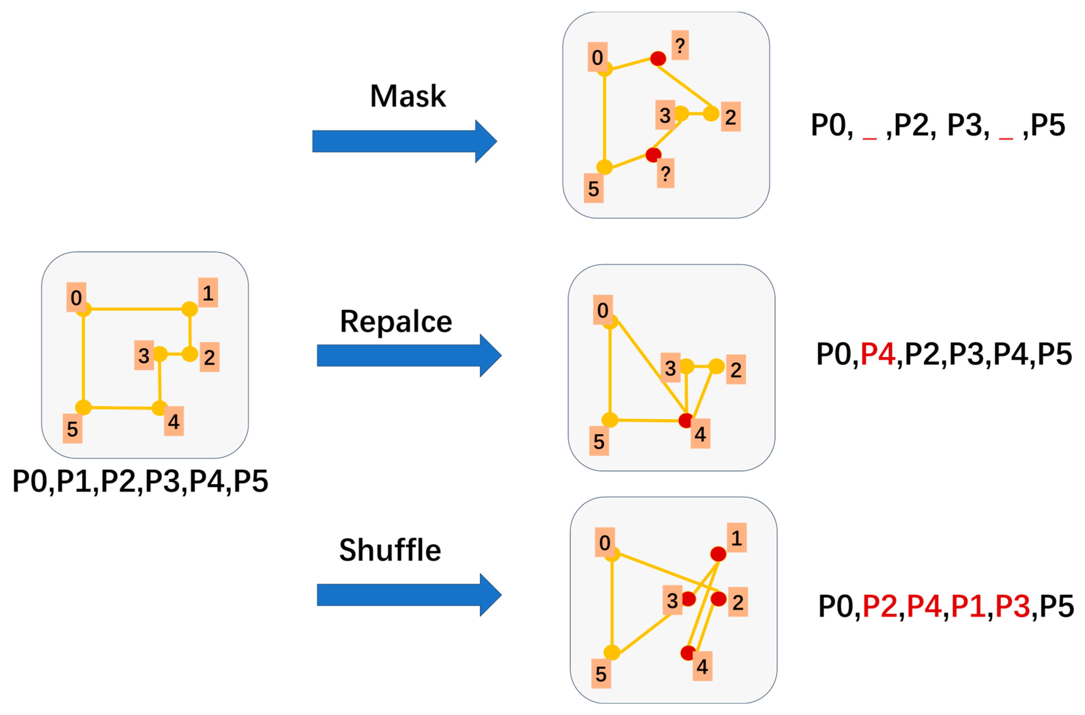
  • Self-supervised reconstruction task: A self-supervised reconstruction task is proposed, wherein the model is trained to reconstruct the original building outline from noise-injected vector sequences. This facilitates the learning of implicit geometric relationships, reduces reliance on labeled data, and enhances training efficiency and model generalization.
  • Comprehensive evaluation: Experiments were conducted with comparative testing and evaluations using several metrics. The results demonstrate TPSM’s superiority in preserving the key characteristics of building outlines.

2. Materials and Methods

To address the limitations of the existing building simplification methods, this study proposes the TPSM, which is inspired by the denoising sequence-to-sequence pre-training method (BART) in the field of natural language processing [28].
This model directly processes the vector coordinate sequences of buildings and generates simplified vector sequences. The model comprises a bidirectional encoder and an autoregressive decoder. This architecture was selected due to its integration of global context understanding, facilitated by the bidirectional encoder, and sequence generation precision, enabled by the autoregressive decoder, both of which are necessary for effective building contour simplification. The encoder’s bidirectional design, implemented through layered Transformer structures, processes the entire input sequence simultaneously. This capability supports the identification of long-range dependencies and the comprehension of the building contour’s overall shape and structure. In contrast, unidirectional encoder alternatives, which rely solely on prior sequence data, are constrained in their capacity to fully represent the contextual information.

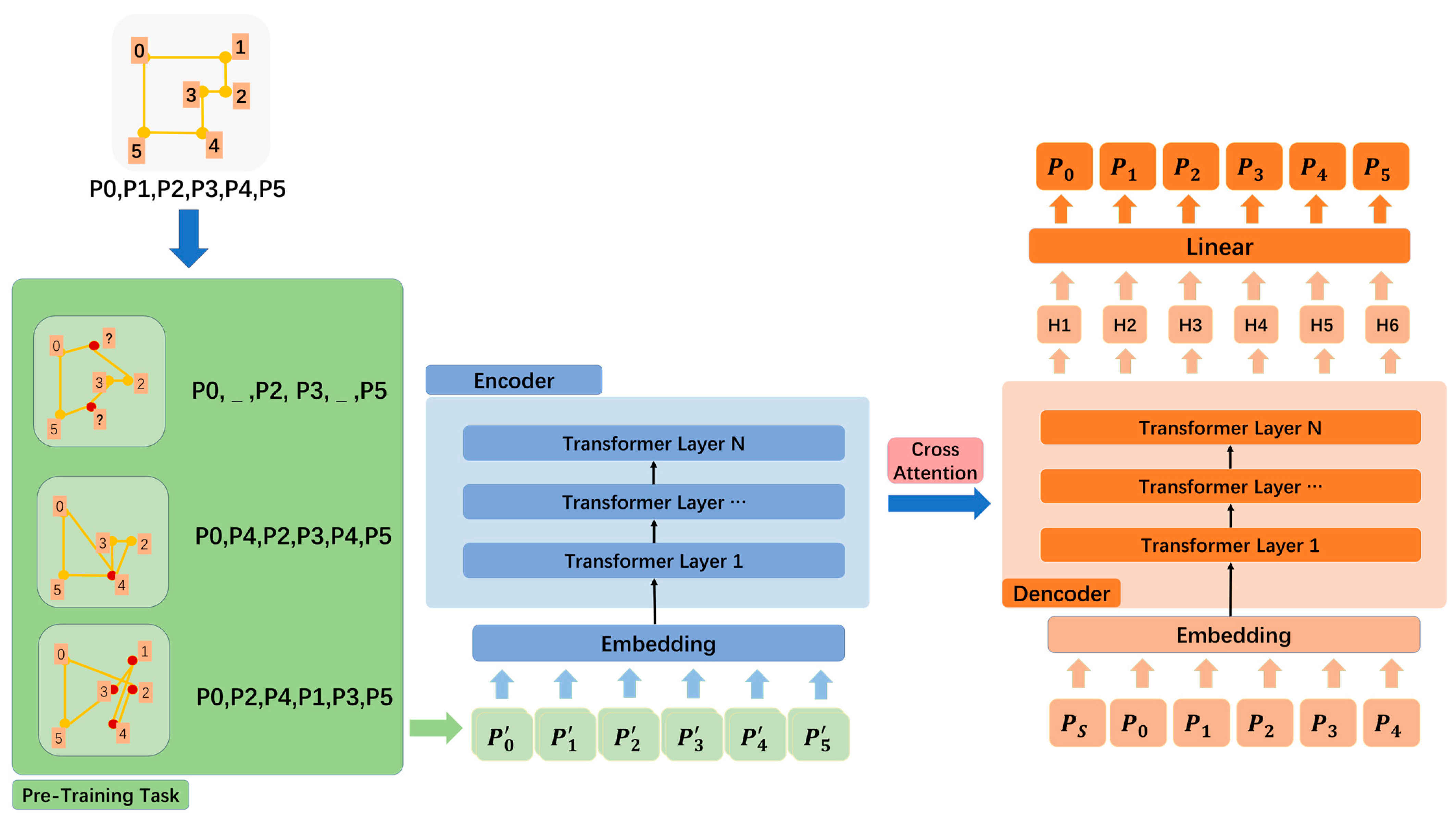
2.1. Model Architecture

The model adopts a Transformer-based encoder–decoder architecture with a multihead self-attention mechanism at its core. The primary components are the input representation, encoder, and decoder, as shown in Figure 2.

2.1.1. Input Representation

The building outlines are represented as an ordered sequence of projected coordinates S = P 1 , P 2 , , P m , where P i = ( X i , Y i ) denotes the projected coordinates (in meters, UTM) of the i-th vertex of the building’s outline. To effectively capture the geometric characteristics of the buildings, the coordinate sequence was transformed into a vector sequence that encompassed both positional and feature embeddings. Positional embeddings provide information about each vertex’s position within the sequence, whereas feature embeddings characterize the geometric features of the outline. These features, learned autonomously by the model, usually manifest as high-dimensional (e.g., 512-dimensional) dense features, distinct from traditionally crafted features, such as angles, area, and principal directions of bounding rectangles.
Positional encoding is crucial because the Transformer model relies on a self-attention mechanism that inherently lacks awareness of the order of the input data. Without positional embeddings, the model views coordinates such as S 1 = P 1 , P 2 , P 3 , , P m and S 2 = P 2 , P m , P 1 , , P 3 as identical, undermining the interpretability of the output shape. It is important to note that positional embedding refers to encoding the order of the coordinates in the sequence, that is encoding 1 , 2 , 3 , , m in P 1 , P 2 , P 3 , , P m , whereas feature embedding pertains to encoding the coordinate values P i X i , Y i .
In contrast to the absolute positional encoding used in the BART model, we employed relative positional encoding to provide positional information for coordinating the sequence inputs. This enhancement allows the model to accommodate sequences of varying lengths better and improves its adaptability to different sequential length distances. Relative positional encoding, which is commonly used in natural language processing, encodes positional information by mapping the positional differences between sequence elements, thereby embedding relative positional relationships within the self-attention mechanism. In this study, we adapted encoding to suit the positional representation of vector polygon sequences.
Consider that, for the i-th vertex, P i X i , Y i , in the sequence, with its feature embedded as x i , and position embedded as p i , the final input representation is x i + p i . When this is used as the input for the Transformer to extract the attention,
q i = x i + p i W Q k j = x j + p j W K v j = x j + p j W V a i , j = s o f t m a x q i k j o i = j a i , j v j
The expansion of q i k j results in:
q i k j = x i W Q W K x j + x i W Q W K p j + p i W Q W K x j + p i W Q W K p j
The term x i W Q W K x j represents attention between inputs that is independent of position, whereas x i W Q W K p j and p i W Q W K x j , respectively, represent the relationships between positional and geometric features within the sequence. This is extremely important for extracting building contour features. Therefore, the value p ~ i j , which is related to relative position, is used to represent p i and p j . The term p i W Q W K p j represents the attention between two positional features, but because the relationship between positions has already been represented by relative position, this part is directly removed. Thus, the positional encoding used in this study is as follows:
q i k j = x i W Q W K x j + p ~ i j W Q W K x j + x i W Q W K p ~ i j
The value of p ~ i j follows the Sinusoidal position encoding [29]:
p ~ i j = P E i j , 2 k = sin p o s 10000 2 k d m o d e l ,
p ~ i j = P E i j , 2 k + 1 = c o s p o s 10000 2 k d m o d e l .
Positional encoding effectively captures the relative positional information, helping the model capture the relative positional relationships between building vertices, learn the relative positional relationships between adjacent vertices, and learn the relative positional relationships between different parts of the building outline, thereby enhancing the performance of the model. In addition, relative positional encoding can better handle long-distance dependencies, allowing it to manage tasks involving more complex building outlines. Absolute position encoding, on the other hand, would assign fixed embeddings to each position, making it difficult for the model to generalize to building contours with different numbers of vertices or to effectively capture the relationships between distant vertices.

2.1.2. Encoder

The encoder captures the global features of the input building vector sequence, whereas the decoder generates a simplified building outline vector sequence. The bidirectional nature of the encoder, achieved through the stacking of Transformer layers, allows it to consider the entire input sequence at once. This is essential for capturing long-range dependencies and understanding the overall shape and structure of the building contour. Alternative architectures, such as a unidirectional encoder, would only have access to past information, limiting their ability to capture the complete context.
In the building simplification task, the input to the encoder was a sequence of coordinates representing the outline of the building. After processing by the encoder, a hidden state vector containing the geometric feature information of the building was obtained. The encoder was designed using six identical Transformer layers stacked together, as shown in Figure 3. Each Transformer layer consists of three parts: a multihead self-attention layer, a fully connected layer, and skip connections with layer normalization.
The input coordinate sequence was processed through the input representation section to obtain two outputs: feature encoding and position encoding. Feature encoding undergoes linear mapping to obtain the query (Q), key (K), and value (V) matrices. The attention weights QKT are calculated according to (3) and position-encoding information, and the attention weights Q K T are calculated. Scaled Dot–Product Attention is used to normalize the attention, and the normalization formula is as follows:
Attention Q , K , V = softmax Q K T d k V .
At this point, the attention of a single head is obtained. The same process was performed in parallel to compute the attention for a total of 12 heads, and the outputs of all heads were concatenated to produce a unified output. The concatenation process is as follows.
M u l t i H e a d Q , K , V = C o n c a t h e a d 1 , h e a d 2 , , h e a d 12 W O .
After concatenating and normalizing the multihead attention, it is passed through two linear layers and a ReLU activation function to serve as the output of the entire Transformer layer. The formula is as follows:
F F N x = m a x 0 , x W 1 + b 1 W 2 + b 2
Residual connections and layer normalization must be added between each sublayer to ensure model stability and accelerate training.

2.1.3. Decoder

The decoder generates a simplified sequence of coordinates S = P 1 X 1 , Y 1 , P 2 X 2 , Y 2 , , P n X n , Y n , where n m , in an autoregressive manner. The structure is composed of six identical Transformer layers stacked together. However, unlike the encoder, the decoder must handle attention from the encoder’s output using cross-attention. Each Transformer layer consists primarily of a masked multihead self-attention mechanism, an encoder–decoder cross-attention mechanism, and a feedforward network with a residual mechanism, as shown in Figure 4.
The decoder is autoregressive when generating a simplified output; therefore, a causal mask is required for multihead attention during the training process to prevent label leakage. The causal mask is shown in Figure 5, where S and E represent the start and end of the sequence, respectively.
The core of the decoder is the cross-attention mechanism with the encoder output, which is a hidden state. Through cross-attention, the model focuses on different parts of the input sequence when generating each output coordinate of the simplified result, allowing it to model the overall structure of the building outline and the relationships between various vertices.
The output of the final layer of the encoder is transformed into key (K) and value (V) matrices. These matrices represent the encoded representation of the input building outline, with each key corresponding to a vertex or feature in the outline and the value containing contextual information about that vertex or feature.
The output of the current layer of the decoder is linearly transformed into a query (Q) matrix that represents the information required by the decoder at the current moment. In the autoregressive decoding process, because of the presence of a causal mask, the query at the current moment can only see the previously generated output vertices. However, because K and V are present in each attention calculation, the complete information of the input outline is used in the decoding process.
The position embedding and attention calculation still use Formula (6), and the feedforward network and residual mechanism are the same as those in the encoder. The output of the decoder is passed to the next step of autoregressive decoding to generate the next output vertex.
Using a causal mask and cross-attention, the decoder can dynamically focus on different parts of the input outline when generating each output vertex. For example, when processing the building corners, the decoder can focus on the vertices near the corners to preserve the shape features of the original building. This repeated use of the encoder output allows the decoder to maintain awareness of the overall building structure during the process of generating a simplified outline, thereby avoiding the global distortion caused by local optimization. Compared with recurrent neural networks [30] and long short-term memory [31], the cross-attention mechanism of the Transformer allows the decoder to directly access any part of the input sequence and better capture long-distance dependencies. This is a key advantage over recurrent architectures, which are prone to vanishing gradients and struggle to effectively model long-range dependencies in sequences. The autoregressive nature of the decoder ensures that the generated sequence is coherent and respects the sequential nature of building contours. Alternative approaches, such as generating the entire sequence at once, would not be able to enforce this sequential constraint and could lead to distorted or invalid building shapes.

2.2. Self-Supervised Reconstruction Task

The self-supervised reconstruction task for building outlines was designed to enable the model to learn the geometric characteristics and simplification rules of building outlines. This task is analogous to the text corruption and repair task in BART. The main idea was to introduce random perturbations into the coordinate sequence of the building outlines, simulate various levels of geometric deformation and data noise, and train the model to reconstruct the original coordinate sequence. The specific methods include vertex masking, vertex replacement, and vertex shuffling, as shown in Figure 6.
Vertex masking: Some vertices of the building were randomly selected and replaced with a special identifier to simulate missing information.
Vertex replacement: Randomly replace some vertices with new, randomly selected points.
Vertex shuffling: Vertices are randomly reordered in the sequence of the building outline, forcing the model to learn the relative positional relationships between the vertices and comprehend the overall shape of the building outline.
The noise perturbation was applied with the following probabilities: vertex masking (15%), vertex replacement (10%), and vertex shuffling (10%). These probabilities were empirically chosen, drawing inspiration from noise settings commonly used in NLP sequence-to-sequence pre-training tasks, such as in BART, and were found to be effective in our preliminary experiments.
The complete workflow of the self-supervised reconstruction task is shown in Figure 7. The original shape coordinates are P 0 , P 1 , P 2 , P 3 , P 4 , P 5 . After preprocessing for pre-training, the sequence becomes [ P 0 , P 1 , P 2 , P 3 , P 4 , P 5 ] . This sequence was input into the Transformer feature-encoding network. Through the encoding, decoding, and cross-attention mechanisms, the decoder outputs predictions targeting the original sequence values P 0 , P 1 , P 2 , P 3 , P 4 , P 5 . It is essential to note that the input to the decoder follows the same structure as that depicted in Figure 4, including sequences P s , P 0 , P 1 , P 2 , P 3 , P 4 and a causal mask. The start token P s prompts the decoder to begin, whereas the causal mask ensures that future parts of the sequence remain unseen during decoding, preventing label leakage. This setup allows the model to predict the entire sequence simultaneously during training, significantly boosting training efficiency by eliminating sequential generation.
There are two reasons for using a self-supervised reconstruction task of building contours to pre-train the model instead of directly simplifying the model through end-to-end training. First, obtaining high-quality paired data from original and simplified building outlines is costly and labor-intensive. Pre-training with a self-supervised task significantly reduced the reliance of the model on labeled data. Second, directly reading the raw coordinate sequence lacks explicit shape features such as angles, curvature, and orientation. The self-supervised reconstruction task based on noise perturbation allows the model to effectively learn these implicit geometric relationships, substantially enhancing the efficiency and generalizability of the subsequent supervised training for simplification tasks at different scales and with varying styles.

2.3. End-to-End Building Simplification

After pre-training, the model acquired the ability to understand and reconstruct building outlines. To achieve end-to-end building simplification, we employed scale-driven simplification as a fine-tuning task. The core idea of this task is to guide the model to simplification using building data at different scales.
End-to-end building simplification uses a model architecture that is essentially the same as the pre-training phase but removes the processing steps of the pre-training task, as shown in Figure 8. The model uses building outlines from large-scale maps as the input and the corresponding simplified outlines from small-scale maps as the target output. It learns mapping from large-to-small-scale outlines using a cross-entropy loss function. During the model training, the input part of the decoder was the same as that in the pre-training phase. However, during model prediction, since the target [ P 0 , P 1 , P 2 , P 3 ] does not exist, an autoregressive approach is needed for decoding. Specifically, a special starting point, P S , is the first input to initiate decoding. After obtaining the first decoding result, P 0 , it was used as an input to decode the model again. At this point, the decoder input is [ P S , P 0 ] , and this process continues until the decoder outputs a special endpoint P E . The complete output at this point is considered to be a simplified result.
By combining the geometric feature reconstruction pre-training task and scale-driven simplification fine-tuning task, the construction of an end-to-end building simplification model was completed.

2.4. Hyperparameter Tuning

The performance of the TPSM model is significantly influenced by several key hyperparameters. To optimize these settings, we conducted a systematic hyperparameter tuning process, where we explored the following hyperparameter ranges:
Encoder/decoder layers: {2, 4, 6}.
Attention heads: {8, 12}.
Hidden layer dimensions: {256, 512, 768}.
Additionally, other hyperparameters were fixed as follows: activation function was set to GELU, dropout rate was uniformly set to 0.1, and both the encoder and decoder feed-forward network dimensions were set to 3072.
A grid search approach was employed to evaluate different combinations of these hyperparameters using a validation dataset. Optimization was carried out using the AdamW optimizer with a learning rate of 5 × 10⁻⁵ and a weight decay of 0.01. A learning rate scheduling strategy was adopted, which involved a linear warm-up phase followed by cosine decay. Model performance was assessed based on both training and validation loss.
The final hyperparameters were selected based on the best performance observed on the validation set, ensuring a balance between model simplification quality and computational efficiency. The optimal configuration, which is further detailed in Section 3.2, provided the best trade-off between performance and computational cost for the task at hand.

3. Results

3.1. Dataset

The dataset used in this study was based on that previously referenced [4], which was collected from a 1:10 k building dataset in Shenzhen, China. As shown in Figure 9, the buildings were simplified to 1:25 K, and these data were used as the target training data. Data with ID mismatches between the source and target data as well as data that could not be matched owing to merging operations were excluded, resulting in a dataset of 2980 pairs of building contour data. The dataset included buildings of varying complexities and shapes. The dataset was randomly divided into a training set of 2000 pairs and a validation set of 980 pairs. Additionally, 1000 building data points were randomly selected from the original collected data as the test set without performing 1:25 k simplified data matching.

3.2. Model Parameter Settings

The TPSM model was implemented using Python 3.8 and PyTorch 1.10. Both the encoder and decoder consist of six layers of Transformer stacks, each containing 12 multihead attentions. The hidden layer encoded the shape features in 768 dimensions, and the feedforward neural network in the encoder–decoder was set to 3072 dimensions. The GELU function was used as the activation function, and the maximum acceptable sequence length was 64. The hardware configuration included 64 GB memory, an AMD R9-5900HX CPU, and an NVIDIA GeForce RTX 3080 laptop.

3.3. Evaluation Metrics

To evaluate the effectiveness of the simplified buildings, a comprehensive set of metrics focusing on position, size, perimeter, shape, and overall generalization quality were employed. The evaluation metrics were as follows:
Position changes were evaluated using the Hausdorff distance (HD). For the original building shape, S = P 1 , P 2 , , P m , and the simplified shape, S = P 1 , P 2 , , P n , the HD between them is defined as
H D S , S = max h S , S , h S , S ,
h ( S , S ) = m a x i 1 , m   { m i n j 1 , n   P i P j } .
The changes in the size of the building before and after the simplification were measured using the area change rate (AC):
A C S , S = A r e a ( S ) A r e a ( S ) × 100 % .
The changes in the perimeter of the building before and after simplification were measured using the perimeter change rate (PC), as follows:
P C S , S = P e r i m e t e r S P e r i m e t e r S × 100 % .
The changes in the shape of the building before and after simplification were represented by the IoU.
I o U S , S = A r e a S S A r e a S S .
To further evaluate the simplification performance, especially considering the generalization quality and regularity of simplified buildings, we introduced C-IoU and Shape Regularity Percent (SRP) as additional evaluation metrics. The degree of simplification is quantified by N-Ratio.
N - r a t i o S , S = N S N S × 100 % .
where N S represents the number of vertices in the original building contour, and N S represents the number of vertices in the simplified building contour. A lower N-Ratio indicates a stronger simplification capability.
Shape Regularity Percent (SRP) quantifies the regularity of the simplified contour. For each interior angle of the simplified polygon, we assess whether its angle is close to 90 or 270 degrees. If the angle deviation from 90 or 270 degrees is below a threshold, the angle is considered a regularized interior angle. SRP is the percentage of regularized interior angles among all interior angles, calculated as follows:
S R P S = a n g l e i S R e g u l a r ( a n g l e i ) N
R e g u l a r a n g l e i = 1 ,     min ( a n g l e i π 2 , a g n l e i 3 2 π ) < θ t h r e d 0 ,     min ( a n g l e i π 2 , a g n l e i 3 2 π ) θ t h r e d
C-IoU assesses the balance between overall performance and contour geometric characteristics. It measures the model’s ability to generate simpler contours while preserving original building details. The calculation formula is as follows:
C - I o U S , S = 1 N G ( S ) I o U ( S , S ) ,
N G S = 1 2 2 1 + e ( k ( N S / N S 0.5 ) ) 1 N S N S .
The metric N G ( S ) represents the complexity of the original contour and the effectiveness of contour simplification, where N S is the number of points in the simplified contour, and N S is the number of points in the original contour. The function N G S takes values between 0 and 0.5. When the simplified contours have a number of points close to that of the original contours, N G S reaches its maximum value of 0.5. This indicates that the original contour may either be simple enough to require no further simplification or that the simplification algorithm failed to significantly reduce the contour complexity. At this point, C-IoU equals half of the IoU. When the simplified contour effectively reduces the number of points in the original contour, it indicates that the original contour is relatively complex, and the algorithm is effective. N G S reaches its minimum value of 0, at which point C-IoU equals IoU. The parameter k can control the optimal simplification ratio, and in the experiment, k is set to 4, resulting in an optimal simplification ratio of 0.5, meaning the simplified contour retains half the points of the original contour. If the simplification is excessive, then the value of N G S will also increase, with a maximum value of 0.25. This metric can effectively sense contour complexity and better measure the simplification performance of the model. By weighting the IoU with 1 N G ( S ) , C-IoU achieves higher scores when the simplification strikes an appropriate balance between preserving shape features (IoU) and controlling polygon complexity (NG). Importantly, C-IoU decreases significantly when the simplified contour either removes too much detail or retains excessive redundant vertices.
These evaluation metrics can be divided into two categories. One category characterizes the quality of the simplified contour, such as AC, PC, and SRP. AC and PC reflect the changes in the area and perimeter of the original contour due to simplification; the closer these two values are to 1, the better the preservation of the contour shape after simplification. SRP indicates the orthogonality of the simplified contour; a lower value signifies better angular orthogonality of the simplified contour. The other category represents the similarity between the simplified contour and the original contour, such as HD and IOU. HD measures shape similarity from the perspective of coordinate distance; a lower value indicates that the simplified shape is closer to the original shape. IoU measures similarity based on the overlap between the simplified and original contours; a higher value indicates a greater degree of overlap between the simplified contour and the original contour.
It is important to note that these metrics alone don’t fully capture cartographic generalization quality. For example, perfect similarity (AC = 1, IoU = 1, PC = 1, HD = 0) would indicate no generalization at all. C-IoU, on the other hand, comprehensively considers the model’s simplification capability based on contour complexity. For contours with high complexity, it assigns greater weight to assess the model’s simplification capability and shape preservation ability. In contrast, simpler contours require less from the simplification capability; in this case, the focus is primarily on the model’s shape preservation ability to determine whether the model can achieve a good balance between simplifying the contour and maintaining its shape.

3.4. Experiments and Analysis

The dataset used for testing contained 1000 samples. Two typical regions were selected to visualize the test dataset, and the results are shown in Figure 10. The evaluation metrics for the results were calculated and are summarized in Table 1 and visualized in Figure 11.
To complement the quantitative evaluations, a subjective assessment of the simplification results was conducted. Three experienced mappers were invited to evaluate a random sample of 100 simplified building contours from the test dataset. Each simplified building was categorized by the mappers as “Good”, “Average”, or “Unacceptable” based on their visual assessment of shape preservation, simplification quality, and overall cartographic suitability.
The results of the subjective evaluation were recorded as follows: 86% of the simplified buildings were rated as “Good”, 13% were rated as “Average”, and 1% were rated as “Unacceptable”. These findings suggest that the TPSM model generally produces simplified building contours that are deemed visually acceptable and cartographically appropriate by experienced map users. The high “Good” rating indicates that the essential characteristics of the building shapes are effectively preserved while a reasonable level of simplification is achieved.
In addition to this qualitative feedback, a transition is made to the quantitative analysis to provide a more comprehensive understanding of the results. From the statistical data in the charts and the visualizations, an analysis of the results reveals the following:
Geometric accuracy: The average area change ratio after simplification was 0.95, with a standard deviation of 0.080; the median value is 0.982, indicating a slight tendency towards area reduction, but with most results close to the original area. The average IoU was 0.901, with a standard deviation of 0.086, and a median of 0.925, showing a high degree of overlap between the simplified and original building shapes. The average perimeter change ratio was 1.026, with a standard deviation of 0.459, and a median of 0.988, suggesting that perimeter is generally well-preserved, although there are instances of increased perimeter. The average HD was 0.314, with a standard deviation of 0.391, and a median of 0.206.
Simplification and regularity: The average N-Ratio was 0.637, indicating a significant reduction in the number of vertices, which confirms the method’s simplification capability. The average Shape Regularity Percent (SRP) was 0.275. It is important to acknowledge that, while SRP aims to quantify the orthogonal nature of the simplified buildings, perfect orthogonality is not always achievable or desirable. Some simplified shapes, such as regular pentagons, Y-shaped outlines, or buildings with genuinely non-orthogonal features, will naturally have lower SRP values. Nevertheless, an SRP of 0.275 is not considered excellent, suggesting that there is still room for improvement in the algorithm’s orthogonalization capabilities.
Comprehensive evaluation: The average C-IoU was 0.735. C-IoU serves as a comprehensive metric, balancing the degree of simplification with the preservation of shape fidelity. A C-IoU of 0.735 suggests a good overall balance between simplification and shape retention.

4. Discussion

4.1. Ablation Studies

To investigate the contribution of key components of TPSM, we conducted a series of ablation studies. We focused on the following components:
Relative position encoding (RPE): The performance of TPSM with RPE was compared to a variant using absolute position encoding (APE). In the APE variant, after embedding the sequence coordinates, the absolute position encoding was computed using Formulas (4) and (5). This encoding was then concatenated with the coordinate embeddings to form the input to the model.
Self-supervised reconstruction (SSR): The performance of the full TPSM model (with SSR pre-training) was compared to a variant trained only on the simplification task without pre-training.
Number of encoder/decoder layers: The performance of TPSM was evaluated with varying numbers of encoder and decoder layers (2, 4, and 6 layers).
The results of the ablation studies are summarized in Table 2.
After replacing RPE with APE, the model performance declined across all metrics, especially in IoU (from 0.901 to 0.855), HD (from 0.314 to 0.496), and C-IoU (from 0.735 to 0.588). The advantage of RPE lies in its ability to capture the relative positional relationships between nodes, which is crucial for generating more orthogonal shapes, especially in architectural contour simplification tasks.
Removing SSR pre-training resulted in a significant performance drop, particularly in IoU (from 0.901 to 0.455), HD (from 0.314 to 1.296), and C-IoU (from 0.735 to 0.283). Additionally, without SSR, the model’s training time greatly increased, and the predicted results became largely unusable. SSR pre-training significantly improved the model’s performance by allowing it to learn latent geometric relationships and simplification rules. Therefore, SSR is a critical component for the success of the model.
The model’s performance significantly improves with the increase in the number of encoder/decoder layers. When using two layers for the encoder/decoder, the performance is poor, with a C-IoU of only 0.135 and an IoU of 0.352. This indicates that the model lacks sufficient parameters to learn effective feature representations, leading to poor performance in the contour simplification task. After increasing to four layers, the performance improves significantly, with C-IoU rising from 0.135 to 0.535 and IoU increasing from 0.352 to 0.791. This shows that the enhanced encoding and decoding capabilities allow the model to learn relevant simplification rules, such as handling straight lines and curves, although there is still room for improvement in detail handling, such as accurately processing corners and curves. When using a six-layer encoder/decoder (the complete model), performance further improves, with C-IoU reaching 0.735 and IoU at 0.901. This indicates that the increase in layers enhances the model’s ability to capture complex data features, but at this point, the performance gains begin to level off, showing that six layers achieve an effective balance between model capacity and computational cost.
These ablation studies provide important insights into the contributions of each key component and demonstrate the rationale behind our design choices for the TPSM.

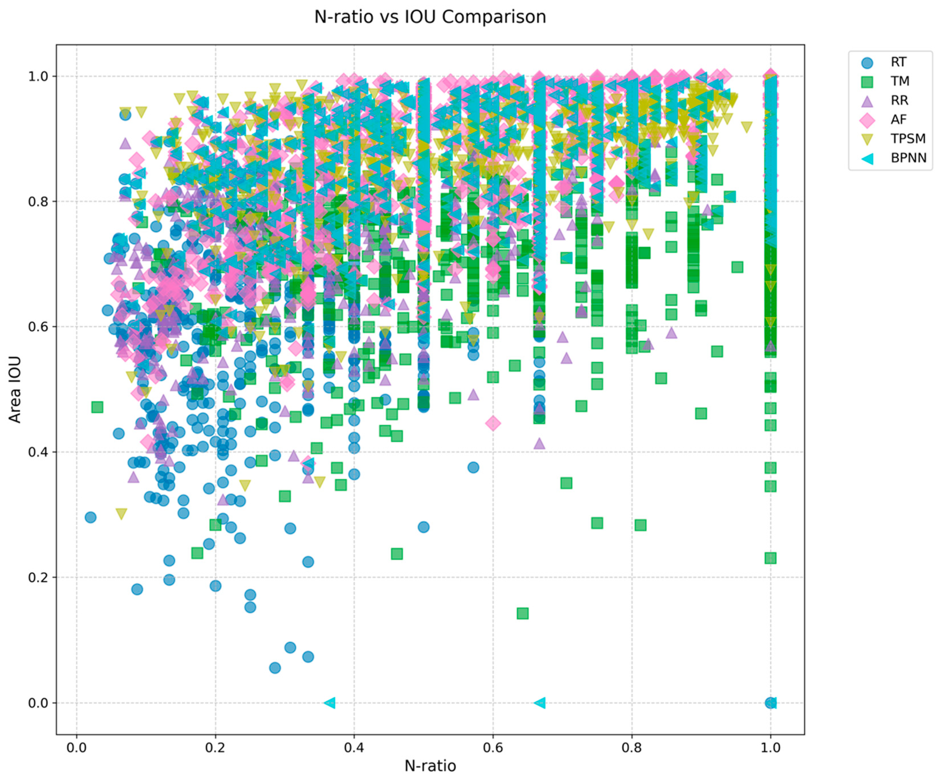
4.2. Comparison and Analysis

To comprehensively evaluate the proposed method, we simplified the original buildings using four rule-based algorithms: rectangle transformation (RT) [32], template matching (TM) [12], adjacent four-points (AF) [15], recursive regression (RR) [17], and a machine learning algorithm based on artificial neural networks (BPNNs) [4]. The results were compared at a 1:25,000 scale. The average values of various evaluation parameters obtained from these simplifications are listed in Table 3.
The table shows that, while BPNN achieves a slightly lower average coordinate displacement (HD), and RT and TM show better preservation of area (AC) and perimeter (PC), respectively, these metrics do not fully capture the generalization performance. Our proposed method achieves the highest IoU, indicating superior shape preservation. Moreover, considering the balance between simplification degree and shape fidelity, our approach demonstrates the highest C-IoU value, signifying a better trade-off between shape retention and complexity reduction compared to other methods.
Although the average values offer an overview of the simplification results, a deeper analysis of the specific distribution of the evaluation metrics for each method is necessary. Therefore, we used violin plots to visualize the evaluation metrics of the six methods, as shown in Figure 12.
Violin plots effectively demonstrate the distribution density, central tendency, and dispersion of data. The overall width of the plot reflects the density of the data distribution; wider sections indicate a higher concentration of data points around a specific value, while narrower sections suggest a sparser distribution. Internally, violin plots also present two statistical measures: the data mean and median. The overall distribution of a violin plot can reflect the stability of a method’s performance. A violin plot with a concentrated distribution typically implies less performance fluctuation and greater robustness.
Based on the data in the table and the distributions shown in the figures, a detailed analysis of the results from six methods will be conducted. First, the performance of each method in terms of geometric accuracy will be analyzed to assess how well the simplified building shapes retain the geometric properties of the original buildings. This includes AC, PC, IoU, and HD.
AC: Overall, the differences among the methods in this metric are minor. Observing Figure 12, it can be seen that the distributions of all methods are concentrated around 1, indicating that each method has good area retention. Specifically, our approach (0.9551) shows slightly more area reduction compared to BPNN (0.9883) and RT (0.9990) but is comparable to TM (0.9666) and AF (0.9696). RT exhibits the smallest area change, possibly due to the use of a simple scaling method to maintain area consistency.
PC: Our approach (0.9641) shows a PC distribution concentrated around 1, indicating good perimeter retention, similar to the BPNN and TM methods. However, from Figure 12, we can see that TM’s distribution is spread between 0.5 and 1.4. Although the average is close to 1, this does not mean it maintains the perimeter well without deformation. On the contrary, since this method uses fixed templates to replace corresponding buildings and can only maintain geometric accuracy through scaling, it is difficult to balance perimeter, IoU, and other metrics while keeping the area consistent, leading to suboptimal results. Methods like RR, AF, and RT also struggle to achieve good perimeter retention, with RT (0.7853) performing poorly in this metric due to its focus on maintaining area.
IoU: This metric reflects the shape similarity between the original and simplified buildings. Our approach (0.9012) outperforms all other methods, indicating excellent shape retention. BPNN (0.8752) and AF (0.8684) also perform relatively well, while RT (0.6981) and TM (0.7298) have significantly lower IoU values.
HD: Lower HD values indicate better positional accuracy. Our approach (0.3132) and BPNN (0.3108) achieve the lowest HD values, demonstrating good performance in minimizing positional differences. RT (0.7370) and TM (0.5973) have significantly higher HD values. The distribution analysis (Figure 12) confirms that our approach, BPNN, and AF have good distributions.
Optimal performance on a single metric does not necessarily indicate overall excellence. Instead, a good generalization balances similarity with a reduction in complexity. For example, simple scaling can ensure that AC is close to 1, as seen with the RT algorithm, and minimizing shape changes can result in a higher IoU. Therefore, the evaluation of simplification methods also needs to consider the simplification rate. Only when effective simplification is achieved while still maintaining good geometric features can a method be considered excellent. Thus, the following analysis will comprehensively consider both the simplification rate and geometric accuracy.
N-Ratio and IoU analysis: The N-Ratio reveals the extent of vertex reduction, while IoU represents the ability of the simplification method to maintain geometric accuracy. By plotting N-Ratio on the x-axis and IoU on the y-axis, we can visualize 1000 simplification results for the six methods, as shown in Figure 13. In the figure, points closer to the top indicate higher geometric accuracy, and points closer to the left indicate a higher degree of simplification. If a method’s points are concentrated in the bottom-left corner, then it is indicated that the method oversimplifies the shapes, as seen with the RT method, which only uses rectangles to simplify building outlines, leading to significant limitations. The TM and RR methods are distributed in the central area of the figure, indicating that these methods have some simplification capability but are not strong in maintaining geometric accuracy. Comparing our approach and BPNN, it is observed that for the same simplification rate, our approach is closer to the top, indicating that it can better maintain geometric features while simplifying.
To quantitatively measure the algorithm’s ability to balance simplification and shape retention, the C-IoU metrics of each model are compared. From the distribution of this metric for each model shown in Figure 12, it can be seen that our approach (0.735) achieves the highest C-IoU score, and its sample distribution is better than that of other methods, indicating that it achieves the best overall balance between simplification and shape retention.
To further validate the performance of the proposed method (TPSM), we conducted paired t-tests comparing the C-IoU values of TPSM against each of the other five methods. The results, shown in Table 4, demonstrate statistically significant differences (p < 0.001) in all cases, with TPSM exhibiting a higher mean C-IoU and substantial effect sizes.
Based on the above analysis, including the statistically significant differences observed in the t-tests, our proposed method and the BPNN method outperformed the rule-based methods (RT, TM, AF, and RR) for building simplification tasks. They demonstrated a better adaptation to diverse building contour types. In terms of preserving the building shape characteristics, the proposed method surpasses the other five methods. Specifically, the approach proposed achieves the best balance between simplification and shape preservation (as reflected in C-IoU).

4.3. Simplification of Buildings with Different Complexities

In the process of simplifying the original buildings, the level of detail required can vary depending on the geometric complexity of the buildings. This lack of uniformity poses a challenge for deep learning network models. The buildings to be simplified are divided into five groups based on their area sizes. The classification standard involved evenly dividing the range between the maximum and minimum area values into five intervals. The sample quantities for each interval are presented in Figure 14.
The five groups contained 333, 404, 200, 54, and 8 samples, corresponding to the area intervals of [150, 380], [380, 963], [963, 2435], [2435, 6160], and [6160, 15579], respectively. Generally, larger buildings with complex contours require stronger simplification capabilities. Experiments were conducted on the five groups using six methods, and the resulting C-IoU distributions are shown in Figure 15. Observing the C-IoU distributions of the different methods across the five groups reveals that TPSM achieves higher C-IoU for simpler shapes, indicating that the size and contour complexity influence the TPSM method. However, the performance decrease in the first three groups was relatively small, and the TPSM maintained a relative advantage over the other methods in terms of C-IoU. A significant drop in performance was observed in the fourth and last groups, particularly for individual shapes. This is because the lengths of some sample sequences in these two groups exceed 64, while the maximum sequence length for training with the TPSM method is 64 points, resulting in a decline in performance. It is important to note that Group 5, representing the most complex building outlines, contains a relatively small number of samples. This limited sample size may contribute to the observed variability in mean C-IoU values for this group, and the results for Group 5.
Figure 16 presents a comparative view of the simplification results for different complexity groups, with scale bars added to each subfigure. Groups 0–4 correspond to the five aforementioned area intervals.
For low-complexity buildings (Groups 0–2), RT and TM exhibit limitations due to their rigid geometric assumptions. RT relies on rectangular approximations, which leads to misalignments when handling irregular shapes with curved or diagonal edges, as shown in examples (a), (b), and (d). Similarly, TM’s dependence on predefined templates results in a low overlap ratio when applied to shapes that do not match the templates. While BPNN dynamically integrates various rule-based strategies, its reliance on fixed training patterns occasionally makes it difficult to fit atypical profiles, as seen in cases (a) and (b). In contrast, TPSM more effectively preserves key geometric features, as confirmed by examples (b), (d), and (f) in Groups 0–2, thanks to its sequence-to-sequence learning framework which can adaptively prioritize significant structural information.
High-complexity buildings in Groups 3–4 reveal the inherent limitations of both rule-based and machine learning approaches. Rule-based algorithms (RR, RT, TM) struggle with complex topologies due to their localized processing. RR’s recursive partitioning fails to preserve global consistency (e.g., examples (c), (e), and (j)), while TM and RT have difficulty handling intricate shapes (e.g., examples (f) and (j)). TPSM performs better in preserving overall shapes but faces two key challenges: (1) truncation errors occur when processing long coordinate sequences (>64 points), leading to the loss of detail in slender structures (e.g., examples (i) and (j)); (2) its generative architecture lacks explicit angle optimization, resulting in slightly insufficient orthogonal regularization compared to BPNN (e.g., examples (g) and (h)). Nevertheless, TPSM’s Transformer-based attention mechanism enables it to effectively balance fidelity and simplification in most cases.

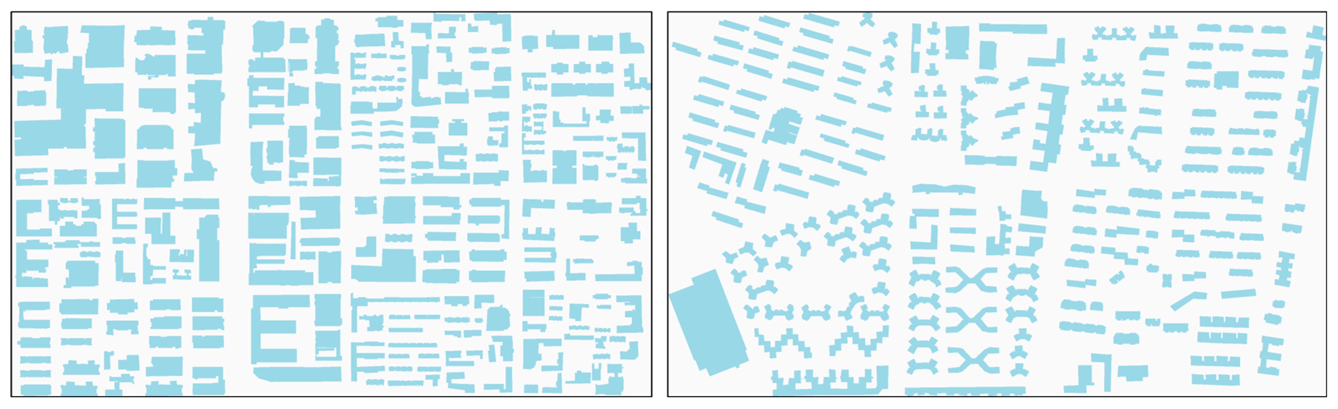
4.4. Cross-Regional Generalization Evaluation

To evaluate the generalization capability of the proposed TPSM model across diverse regions and building characteristics, additional experiments were conducted using a dataset from a different geographical context. Specifically, we utilized the Stuttgart building dataset from the work of Zhiyong Zhou [33], which consists of building polygons sourced from OpenStreetMap (OSM) at an approximate scale of 1:5000. The target map scale for simplification was set to 1:10,000. This dataset includes 1731 buildings of various types from Stuttgart, Germany, which were used as the test set without additional training on this specific data. This approach allows for a direct assessment of the model’s generalization ability to unseen data from a different region. Figure 17 shows the contour simplification results of some buildings in the Stuttgart dataset. The figures visualize the simplification results for contours with smaller areas and contours with larger areas, respectively. It can be observed that the TPSM achieves a good balance between the degree of simplification and similarity for contours of varying shapes and complexities. This performance is consistent with the results on the Shenzhen dataset.
The TPSM model was applied to the Stuttgart dataset, and the results were quantitatively analyzed using HD, AC, PC, IoU, SRP, N-Ratio, and C-IoU. The statistical summary of the evaluation metrics is presented in Table 5.
The results indicate that the TPSM model maintains relatively consistent performance on the Stuttgart dataset, with mean values of AC, IoU, and PC close to those observed in the Shenzhen dataset. Specifically, an average AC of 0.980 indicates excellent preservation of building area, while an average IoU of 0.947 suggests a high degree of shape similarity between the original and simplified buildings. An average HD of 0.306 reflects minimal positional deviation, and an N-Ratio of 0.716 indicates that the model effectively simplified the contours. The SRP value of 0.098 also suggests that the model’s simplification results maintain good orthogonality. Furthermore, a C-IoU of 0.782 further confirms the model’s ability to effectively balance simplification and shape fidelity.
The performance of TPSM on the Stuttgart dataset demonstrates its robustness and generalization capability across different geographical regions and architectural features. Despite differences in architectural styles and map scales between Shenzhen and Stuttgart, the model still maintains a relatively consistent simplification capability, indicating that the simplification rules learned by the model are not overly specific to the training data and can be effectively applied to new, unseen datasets.

4.5. Limitations

Experiments and evaluations using various metrics demonstrated that the proposed TPSM method is effective for building outline simplification tasks of diverse complexities and scales. Compared to traditional rule-based and machine-learning-based methods, TPSM can be directly applied to vector sequences without requiring preprocessing steps such as rasterization or statistical feature extraction. This reduces the number of processing steps and minimizes potential information loss during data conversion. Moreover, its Transformer-based architecture leverages sequence-to-sequence learning to adaptively prioritize significant structural information, enabling robust performance across diverse building types, as evidenced by its high C-IoU scores in both the Shenzhen and Stuttgart datasets. However, the model may still exhibit performance degradation in certain extreme cases, as illustrated in Figure 18. Figure 18a represents a normal simplification result, while Figure 18b–d depict cases where the simplification was less effective. Through detailed analysis, we identified three main categories of challenging samples:
Buildings with more than 64 points (Figure 18b): The current model architecture limits the input sequence length to 64 points to improve training efficiency. Although it is theoretically possible to support longer sequences by adjusting parameters, this requires retraining the entire model, which is computationally expensive. When the number of points in the original building shape exceeds this limit, the model truncates the sequence, leading to a loss of shape details and resulting in simplification errors.
Rare building shapes in the training set (Figure 18c): For building shapes that rarely appear in the training set, the model’s performance is constrained by the scarcity of such samples in the training data. Since TPSM employs a generative approach similar to AIGC (artificial-intelligence-generated content), the model struggles to learn effective simplification rules for these rare cases, resulting in suboptimal simplification outcomes.
Non-traditional buildings with internal cavities (Figure 18d): For buildings with complex topological structures, such as those with internal cavities, the scarcity of such samples in the training data similarly limits the model’s learning capability, preventing it from fully grasping the generation rules for these shapes.
Orthogonal control is an important aspect of building simplification. However, in current generative models, there is no explicit model to impose constraints on it, even though these models can learn certain geometric features from data. Introducing explicit geometric constraints into the loss function could potentially enhance the model’s ability to maintain orthogonality during the simplification process.
To address the above limitations, future work can focus on the following directions:
Sequence length limitation: To improve training efficiency, the input sequence length was limited to 64 points during model training. The model architecture can support longer-sequence inputs. Based on the requirements of the specific tasks, changing the corresponding parameters can achieve longer-sequence-processing capabilities. However, the entire model must be retrained to accommodate this change.
Complex topology: The model currently exhibits poor simplification results for complex topologies, including both long sequence inputs and inputs with holes. Buildings of this type, such as churches, large stadiums, exhibition centers, and special buildings, are typically scarce. This scarcity hindered the ability of the model to learn effective simplified knowledge from these examples. Deliberately collecting and increasing the number of samples can improve the ability of the model to simplify such buildings to a certain extent.
Orthogonality control: Orthogonal control is a key consideration in the simplification process. By designing appropriate loss functions or training tasks that incorporate geometric constraints into the loss function, the model’s performance can be improved. Another promising avenue is to investigate hybrid approaches, combining TPSM with rule-based methods or other preprocessing techniques. For instance, TPSM’s output could be further refined using rule-based methods to enforce stricter orthogonality or handle specific topological constraints.

5. Conclusions

Research on building simplifications directly from vector maps using deep learning is a promising direction, although current solutions are limited. This paper introduces a Transformer-based building simplification model (TPSM) that directly extracts features from building contour vector sequence data, thereby avoiding additional computational overhead and information loss associated with rasterization and statistical feature extraction.
The TPSM improves position encoding by integrating it into a multihead attention mechanism, enabling the efficient extraction of shape and positional features. Through a self-supervised reconstruction task, the model can be pre-trained without supervision, making it possible to fine-tune it with fewer labeled data for specific simplification tasks. This foundation allowed the model to adapt to various scales and simplification styles.
The experimental results demonstrate that the TPSM can handle buildings of varying complexity while preserving the original building shapes in the simplification task. The simplification results are characterized by a high IoU and a low HD, although the method has certain limitations in maintaining the orthogonal properties for complex buildings.
This approach represents a valuable exploration of deep learning for simplifying automated buildings. Beyond its technical contributions, TPSM holds potential for real-world applications, such as urban planning, where simplified building contours can streamline land use analysis, or GIS systems, where efficient vector processing enhances map generalization workflows. Future research could enhance the control of the model over angular orthogonality by introducing geometric feature constraints into the loss function, constructing larger, more representative datasets to improve the performance of complex buildings, and exploring integration with other map generalization operations, such as merging and typification, to develop a more comprehensive automated map generalization solution.

Author Contributions

Conceptualization, Longfei Cui and Haizhong Qian; Data curation, Lin Jiang and Junkui Xu; Formal analysis, Longfei Cui and Lin Jiang; Methodology, Longfei Cui, Junkui Xu and Haizhong Qian; Software, Longfei Cui; Supervision, Haizhong Qian; Validation, Longfei Cui; Writing—original draft, Longfei Cui; Writing—review and editing, Longfei Cui, Junkui Xu, and Haizhong Qian. All authors have read and agreed to the published version of the manuscript.

Funding

This research was funded by The National Natural Science Foundation of China, grant number 42271463, 42101453.

Data Availability Statement

The code and data of this study will be publicly available on the following page: github.com/GisHED/BuildingSimply (accessed on 23 February 2025).

Conflicts of Interest

The authors declare no conflicts of interest.

References

  1. Touya, G. Multi-criteria geographic analysis for automated cartographic generalization. Cartogr. J. 2022, 59, 18–34. [Google Scholar] [CrossRef]
  2. Steiniger, S.; Weibel, R. Relations among map objects in cartographic generalization. Cartogr. Geogr. Inf. Sci. 2007, 34, 175–197. [Google Scholar] [CrossRef]
  3. Zhao, W.; Persello, C.; Stein, A. Building outline delineation: From aerial images to polygons with an improved end-to-end learning framework. ISPRS J. Photogramm. 2021, 175, 119–131. [Google Scholar] [CrossRef]
  4. Yang, M.; Yuan, T.; Yan, X.; Ai, T.; Jiang, C. A hybrid approach to building simplification with an evaluator from a backpropagation neural network. Int. J. Geogr. Inf. Sci. 2022, 36, 280–309. [Google Scholar] [CrossRef]
  5. Yan, X.; Yang, M. A deep learning approach for polyline and building simplification based on graph autoencoder with flexible constraints. Cartogr. Geogr. Inf. Sci. 2024, 51, 79–96. [Google Scholar] [CrossRef]
  6. Jiang, B.; Xu, S.; Li, Z. Polyline simplification using a region proposal network integrating raster and vector features. GISci. Remote Sens. 2023, 60, 2275427. [Google Scholar] [CrossRef]
  7. Courtial, A.; Touya, G.; Zhang, X. Constraint-based evaluation of map images generalized by deep learning. J. Geovisualization Spat. Anal. 2022, 6, 13. [Google Scholar] [CrossRef]
  8. Douglas, D.H.; Peucker, T.K. Algorithms for the reduction of the number of points required to represent a digitized line or its caricature. Cartographica 1973, 10, 112–122. [Google Scholar] [CrossRef]
  9. Li, Z.; Openshaw, S. Algorithms for automated line generalization based on a natural principle of objective generalization. Int. J. Geogr. Inf. Syst. 1992, 6, 373–389. [Google Scholar] [CrossRef]
  10. Visvalingam, M.; Whyatt, J.D. Line generalisation by repeated elimination of points. Cartogr. J. 1993, 30, 46–51. [Google Scholar] [CrossRef]
  11. Rainsford, D.; Mackaness, W. Template matching in support of generalisation of rural buildings. In Proceedings of the Advances in Spatial Data Handling; Richardson, D.E., van Oosterom, P., Eds.; Springer: Berlin/Heidelberg, Germany, 2002; pp. 137–151. [Google Scholar] [CrossRef]
  12. Yan, X.; Ai, T.; Zhang, X. Template matching and simplification method for building features based on shape cognition. ISPRS Int. J. Geo Inf. 2017, 6, 250. [Google Scholar] [CrossRef]
  13. Wang, L.; Guo, Q.; Liu, Y.; Sun, Y.; Wei, Z. Contextual building selection based on a genetic algorithm in map generalization. ISPRS Int. J. Geo Inf. 2017, 6, 271. [Google Scholar] [CrossRef]
  14. Qingsheng, G.; Jianhua, M. The method of graphic simplification of area feature boundary with right angles. Geo Spat. Inf. Sci. 2000, 3, 74–78. [Google Scholar] [CrossRef]
  15. Wenshua, X. Simplification of building polygon based on adjacent four-point method. Acta Geod. Cartogr. Sin. 2013, 42, 929–936. [Google Scholar]
  16. Sester, M. Optimization approaches for generalization and data abstraction. Int. J. Geogr. Inf. Sci. 2005, 19, 871–897. [Google Scholar] [CrossRef]
  17. Bayer, T. Automated building simplification using a recursive approach. In Cartography in Central and Eastern Europe: CEE 2009; Gartner, G., Ortag, F., Eds.; Springer: Berlin/Heidelberg, Germany, 2009; pp. 121–146. [Google Scholar] [CrossRef]
  18. Haunert, J.-H.; Wolff, A. Optimal and topologically safe simplification of building footprints. In Proceedings of the 18th SIGSPATIAL International Conference on Advances in Geographic Information Systems, San Jose, CA, USA, 2–5 November 2010; ACM: New York, NY, USA, 2010; pp. 192–201. [Google Scholar] [CrossRef]
  19. Duan, P.; Qian, H.; He, H.; Xie, L.; Luo, D. A Line Simplification method based on support vector machine. Geomat. Inf. Sci. Wuhan Univ. 2020, 45, 744–752, 783. [Google Scholar] [CrossRef]
  20. Yan, X.; Ai, T.; Yang, M.; Yin, H. A graph convolutional neural network for classification of building patterns using spatial vector data. ISPRS J. Photogramm. 2019, 150, 259–273. [Google Scholar] [CrossRef]
  21. Cheng, B.; Liu, Q.; Li, X.; Wang, Y. Building simplification using backpropagation neural networks: A combination of cartographers’ expertise and raster-based local perception. GIScience Remote Sens. 2013, 50, 527–542. [Google Scholar] [CrossRef]
  22. Sester, M.; Feng, Y.; Thiemann, F. Building generalization using deep learning. Int. Arch. Photogramm. Remote Sens. Spat. Inf. Sci. 2018, XLII-4, 565–572. [Google Scholar] [CrossRef]
  23. Feng, Y.; Thiemann, F.; Sester, M. Learning cartographic building generalization with deep convolutional neural networks. ISPRS Int. J. Geo Inf. 2019, 8, 258. [Google Scholar] [CrossRef]
  24. Courtial, A.; El Ayedi, A.; Touya, G.; Zhang, X. Exploring the potential of deep learning segmentation for mountain roads generalisation. ISPRS Int. J. Geo Inf. 2020, 9, 338. [Google Scholar] [CrossRef]
  25. Courtial, A.; Touya, G.; Zhang, X. Deriving map images of generalised mountain roads with generative adversarial networks. Int. J. Geogr. Inf. Sci. 2023, 37, 499–528. [Google Scholar] [CrossRef]
  26. Du, J.; Wu, F.; Xing, R.; Gong, X.; Yu, L. Segmentation and sampling method for complex polyline generalization based on a generative adversarial network. Geocarto Int. 2022, 37, 4158–4180. [Google Scholar] [CrossRef]
  27. Yu, W.; Chen, Y. Data-driven polyline simplification using a stacked autoencoder-based deep neural network. Trans. GIS 2022, 26, 2302–2325. [Google Scholar] [CrossRef]
  28. Lewis, M.; Liu, Y.; Goyal, N.; Ghazvininejad, M.; Mohamed, A.; Levy, O.; Stoyanov, V.; Zettlemoyer, L. BART: Denoising sequence-to-sequence pre-training for natural language generation, translation, and comprehension. In Proceedings of the 58th Annual Meeting of the Association for Computational Linguistics, Online, 5–10 July 2020; Jurafsky, D., Chai, J., Schluter, N., Tetreault, J., Eds.; Association for Computational Linguistics: Stroudsburg, PA, USA, 2020; pp. 7871–7880. [Google Scholar] [CrossRef]
  29. Vaswani, A.; Shazeer, N.; Parmar, N.; Uszkoreit, J.; Jones, L.; Gomez, A.N.; Kaiser, Ł.; Polosukhin, I. Attention is all you need. In Proceedings of the 31st International Conference on Neural Information Processing Systems, Long Beach, CA, USA, 4–9 December 2017; Curran Associates Inc.: Red Hook, NY, USA, 2017; pp. 6000–6010. [Google Scholar]
  30. Salem, F.M. Recurrent neural networks (RNN). In Recurrent Neural Networks: From Simple to Gated Architectures; Salem, F.M., Ed.; Springer International Publishing: Cham, Switzerland, 2022; pp. 43–67. [Google Scholar] [CrossRef]
  31. Dyer, C.; Ballesteros, M.; Ling, W.; Matthews, A.; Smith, N.A. Transition-Based Dependency Parsing with Stack Long Short-Term Memory. In Proceedings of the 53rd Annual Meeting of the Association for Computational Linguistics and the 7th International Joint Conference on Natural Language Processing (Volume 1: Long Papers), Beijing, China, 26–31 July 2015; Zong, C., Strube, M., Eds.; Association for Computational Linguistics: Beijing, China, 2015; pp. 334–343. [Google Scholar] [CrossRef]
  32. Wang, Z.; Lee, D. Building simplification based on pattern recognition and shape analysis. In Proceedings of the 9th International Symposium on Spatial Data Handling, Beijing, China, 10–12 August 2000; pp. 58–72. [Google Scholar]
  33. Zhou, Z.; Fu, C.; Weibel, R. Move and remove: Multi-task learning for building simplification in vector maps with a graph convolutional neural network. ISPRS J. Photogramm. Remote Sens. 2023, 202, 205–218. [Google Scholar] [CrossRef]
Figure 1. Illustrative examples of building outline imperfections. (a) Original remote sensing image. (b) Extracted building outlines, with red boxes highlighting typical defects such as jagged edges and blurred corners.
Ijgi 14 00124 g001
Figure 2. Transformer-based Polygon Simplification Model (TPSM).
Ijgi 14 00124 g002
Figure 3. Encoder network architecture.
Ijgi 14 00124 g003
Figure 4. Decoder network architecture.
Ijgi 14 00124 g004
Figure 5. Causal mask (Different corner points in the outline are numbered sequentially, with S and E indicating the start and end of the sequence, respectively).
Ijgi 14 00124 g005
Figure 6. Transformations for noising the input shape (Perturbed points are indicated in red).
Ijgi 14 00124 g006
Figure 7. Network architecture for self-supervised reconstruction tasks.
Ijgi 14 00124 g007
Figure 8. Network architecture for end-to-end building simplification.
Ijgi 14 00124 g008
Figure 9. City architecture dataset illustration.
Ijgi 14 00124 g009
Figure 10. Simplification results using the proposed approach.
Ijgi 14 00124 g010
Figure 11. Scatter plots of evaluation metrics (AC, IoU, PC, and HD) for building simplification results.
Ijgi 14 00124 g011
Figure 12. Violin plots comparing distribution of AC, SRP, IoU, and HD metrics for six simplification methods.
Ijgi 14 00124 g012
Figure 13. A scatter plot analysis of N-Ratio and IoU across six methods.
Ijgi 14 00124 g013
Figure 14. Histogram of the number of different building area categories.
Ijgi 14 00124 g014
Figure 15. C-IoU metric for different methods across varying area groups.
Ijgi 14 00124 g015
Figure 16. Comparison of simplification results for different methods across varying complexity groups (scale bars as meters). Subplots (aj) represent different examples of building outlines across varying complexity groups to illustrate simplification outcomes.
Ijgi 14 00124 g016
Figure 17. Visualization of simplified building contours in the Stuttgart dataset.
Ijgi 14 00124 g017
Figure 18. TPSM simplification results for complex building shapes. (a) Example of successful simplification. (b) Simplification of a building with more than 64 points. (c) Simplification of a building shape rarely seen in the training dataset. (d) Simplification of a building with internal holes.
Ijgi 14 00124 g018
Table 1. Statistical summary of evaluation metrics.
METRICACIoUPCHDN-RatioSRPC-IoU
MEAN0.9550.9011.0260.3140.6370.1520.735
MEDIASN0.9820.9250.9880.2060.6670.1240.779
STD. DEV.0.0810.0860.4590.3910.230.1810.211
Table 2. Results of ablation studies.
Model VariantACIoUPCHDN-RatioSRPC-IoU
TPSM (Full)0.9550.9011.0260.3140.6370.1520.735
TPSM (APE)0.9210.8550.9320.4960.7310.3580.588
TPSM (No SSR)0.6410.4550.911.2960.3740.6580.283
TPSM (2 Encoder/Decoder)0.5550.3520.8262.3140.7850.7720.135
TPSM (4 Encoder/Decoder)0.8950.7911.1310.5140.7790.3020.535
Table 3. Evaluation results of different methods and TPSM.
ScaleMeasureOur ApproachBPNNRTTMAFRR
1:25 kHD0.31320.31080.73700.59730.36850.4190
AC0.95510.98830.99900.96660.96960.9405
PC0.96410.94670.78530.98100.89970.8738
IoU0.90120.87520.69810.72980.86840.8019
N-Ratio0.6370.5560.30.6790.480.425
SRP0.1520.04100.0340.1330
C-IoU0.7350.6540.3760.5720.6090.525
Table 4. T-test results comparing C-IoU of TPSM with those of other methods.
ComparisonTest Statisticp-ValueEffect SizeMean (TPSM)Mean (Other)Std (TPSM)
vs. BPNN8.7315<0.0010.39080.73540.65380.211
vs. AF13.3684<0.0010.59830.73540.60860.211
vs. RT40.293<0.0011.80330.73540.37580.211
vs. RR21.214<0.0010.94950.73540.5250.211
vs. TM18.3082<0.0010.81940.73540.57210.211
Table 5. Statistical summary of evaluation metrics on Stuttgart dataset.
METRICACIoUPCHDN-RatioSRPC-IoU
MEAN0.980.9470.9880.3060.7160.0980.782
MEDIASN0.9730.9580.9980.1380.7320.1010.812
STD. DEV.0.040.0560.1090.220.2270.1720.151
Disclaimer/Publisher’s Note: The statements, opinions and data contained in all publications are solely those of the individual author(s) and contributor(s) and not of MDPI and/or the editor(s). MDPI and/or the editor(s) disclaim responsibility for any injury to people or property resulting from any ideas, methods, instructions or products referred to in the content.

