Abstract
Integrating cyberspace and geographic space through map visualization is a valuable approach for revealing distribution patterns and relational dynamics in cyberspace. The interdisciplinary integration of network science and geographic science has gained increasing attention in recent years. However, current geographic information data models are not suitable for representing cyberspace features and their relations, and there is a lack of general and systematic cyberspace map visualization methods. To address these problems, this paper introduces an integrated data model that aligns spatial and cyberspace features based on a “proxy mode”. This model is designed to support both the visualization of data maps and the analysis of complex networks and graph layouts. In addition, a framework for cyberspace map visualization is introduced, comprising three main stages: “cyberspace data processing”, “cyberspace data rendering”, and “base map processing and map layout”. Using the Routers, BrightKite, and Cables datasets, we developed a web-based CMV system and generated a statistical map, a node-link map, an edge bundling map, a flow map, and a feature distribution map. The experimental results showed that the proposed data model and method framework can be effectively applied to represent the distribution and relations of cyberspace features and help reveal the interaction patterns between cyberspace and geographic space.
1. Introduction
With the rapid development of technologies such as the internet, the Internet of Things (IoT), and mobile communications, cyberspace has become the “second living space” for human production activities, complementing the traditional physical domains of land, sea, air, and outer space. Cyberspace is now considered the fifth strategic domain [1], playing a vital role in social, political, economic, and military fields. Cyberspace can be understood in both narrow and broad senses. Narrowly, cyberspace refers to internet space where humans can access the internet through computers or mobile devices [2]. Broadly, cyberspace refers to networks that connect various information technology infrastructures, including the internet, telecommunication networks, sensor networks, IoT, various computer systems, and virtual human interactions [3]. This paper focuses on the map visualization of cyberspace in its broad sense.
As an effective way to understand cyberspace, cyberspace map visualization (CMV), also known as cyberspace cartography, has become a research hotspot in fields such as geographic information science, network information science, computer science, and social science [3,4,5]. The concept of cybercartography was first introduced by [6], though it differs from the CMV concept discussed in this paper, which aligns more closely with the concepts proposed by [3,5,7,8]. These approaches focus on methods and techniques for representing cyberspace features and their relations within geographic space. Through CMV, cyberspace can be integrated with physical space by mapping virtual positions to actual spatial coordinates. Additionally, this visualization technique facilitates a more intuitive understanding of the structure and characteristics of cyberspace, thereby supporting in-depth analysis of the relationship between cyberspace and physical space.
The earliest map describing cyberspace infrastructure dates back to 1853, illustrating telegraph stations across the United States, Canada, and Nova Scotia [9]. The first conceptual map of the internet’s information space was created by December, a communications company president, at the end of 1994 [10]. Subsequently, an increasing number of experts and scholars have conducted research on how to effectively represent cyberspace features and phenomena in geographic space. Based on their relevance to geographic space, these studies can be broadly divided into the following two directions:
- CMV strongly correlated with geographic space.
This approach employs symbols with specific spatial locations to represent the distribution of cyberspace features in geographic space. Examples include the Advanced Research Projects Agency Network (ARPANET) and internet development maps, submarine fiber optic cables maps (TeleGeography), and internet exchange center maps [9]. Tsou et al. [11] visualized and analyzed viewpoints and events in cyberspace by leveraging IP addresses. Wang et al. [12] mapped the global resource distribution of cyberspace at both the AS and IP levels, while Chen [13] described the basic process of cyberspace cartography and drew a map of network-server operating-system distributions in a certain region. He [14] proposed focusing on critical business networks and important target networks in the power industry and constructed a cyberspace map for the power network. This map accurately represents key objects, node attributes, basic services, and network topological structures. Zhu [15] studied CMV methods from three aspects: cyberspace models, cartographic data, and cyberspace terrains. Zhang [16] proposed a conceptual model suitable for cyberspace maps and comparatively analyzed typical cyberspace maps. To address issues in cyberspace maps such as unclear representation features, inconsistent symbol design standards, and unstandardized visualization methods, Jiang [17] investigated the theories, methods, and key techniques of CMV using cartographic approaches. Zhang et al. [18] proposed a method for simplifying cyberspace data that effectively reduces complexity while preserving key features and accounting for spatial distribution and network characteristics.
- CMV weakly correlated with geographic space.
This method schematically represents information such as cyberspace features that do not have specific spatial locations or whose spatial locations are not important in cyberspace and their relations. Examples include flow maps, cartograms, and network maps. Flow maps represent the direction, flow, and type of cyberspace features from a relatively macro perspective by processing linear symbols through smoothing [19], aggregation [20], layout [21], rendering [22], and generalization [23]. Cartograms use mathematical rules to simplify or distort geographic space to represent specific cyberspace information. For example, Wang et al. [24] proposed a method for cyberspace information map visualization based on a composite distance cartogram, and Liu et al. [25] proposed a visualization method for cyberspace metaphor using the Gosper map. Network maps treat cyberspace as a graph model composed of nodes and edges and represent it in geographic space. There has been extensive research on network maps. Representative methods include force-directed edge bundling [26], skeleton-based edge bundling [27], and kernel density estimation-based edge bundling [28] for network map visualization. Notably, Zou et al. [29] proposed a method for displaying local relational information in cyberspace by creating a local visual space, offering a new approach for CMV. In addition, Jiang et al. [30] proposed a metaphorical visualization framework for cyberspace maps, providing a comprehensive and intuitive visualization method for understanding the interaction between geographic space and cyberspace through a “object–virtual object–process–decision” hierarchical modeling method. Building upon the framework proposed by Jiang, Si et al. [31] developed a GMap-based metaphorical map of network potential.
It is evident that many experts and scholars have been committed to effectively representing cyberspace features or phenomena within geographic space and have achieved useful results. Nevertheless, the above studies still have the following problems. First, most methods for CMV only target specific data types and application scenarios. Thus, there is a lack of a general and systematic method framework for CMV. Second, the existing geographic information data models are not suitable for representing cyberspace features and their relations, necessitating the construction of a data model for CMV. It has been demonstrated that the above problems have gradually become key issues restricting the effective representation of cyberspace in geographic space. To address these problems, this paper introduces a data model and method framework for the visual representation of cyberspace maps. The specific contributions and innovations are as follows:
- The relevant theory of CMV is further improved. Based on the results of existing studies, a conceptual definition and a classification system of CMV are provided, and a symbol system for CMV is established.
- An integrated data model that couples spatial features and cyber features is designed. This model can support not only map visualization but also complex network analysis and graph layouts.
- A method framework for CMV is proposed. This method can effectively represent the distribution and relations of cyberspace features and also help reveal the rules of interaction between cyberspace and geographic space.
2. Basic Theory of CMV
Compared with traditional maps, cyberspace maps differ in terms of content representation, constituent features, and symbol systems. The latter emphasizes the representation of physical or virtual features and their relations in cyberspace, such as the relation network, information flow, and topological structure [13], while the former focuses on the representation of the distribution patterns of geospatial features and has a relatively mature theoretical base and a rich symbol system [32].
2.1. Definition and Classification
To date, a unified description and definition of CMV has not been established. In his doctoral dissertation, Dodge [33] classified cyberspace map visualization into three categories: “maps in cyberspace”, “maps of cyberspace”, and “maps for cyberspace”. “Maps in cyberspace” is similar to the concept of cybercartography proposed by Taylor [6], which mirrors traditional maps, differing only in the media carrying the content. Jiang et al. [34] defined CMV as a map used to visualize information such as physical locations and traffic conditions in cyberspace, aligning with the concept of “maps for cyberspace”. Ai [35] defined CMV as a specialized visualization technique that visually represents the objects, phenomena and processes in cyberspace, serving navigation and analysis within virtual spaces, similar to the concept of “maps in cyberspace”. With the development of information technology and changes in application needs, these definitions have expanded, and the above concepts are no longer suitable for summarizing the current understanding of CMV.
To this end, the present study provides the following updated definition: CMV is a thematic map that visually represents the spatial distribution, relationships, quality and quantity, and flow trends of cyberspace features or phenomena using graphic images in combination with symbolic languages such as charts and texts in a descriptive, generalized, or schematic manner.
In this study, the characteristics of existing cyberspace maps are comprehensively analyzed and categorized into feature distribution maps, node-link maps, statistical thematic maps, and cartogram maps of cyberspace. The explanation of various types of cyberspace maps, along with example maps, is shown in Table A1.
The feature distribution map precisely represents the spatial distribution of cyberspace elements using accurate coordinates. It demands both the precise representation of node element locations and edge element positions. For example, the DNS distribution in San Francisco can be visualized using a point distribution map, the global submarine optical cable distribution can be visualized through a line distribution map, and the distribution of inland communication trunk lines and base stations can be visualized via a point and line distribution map.
In general, node-link maps do not require the precise spatial positioning of nodes or edges. Consequently, nodes can be aggregated and edges bundled to more clearly represent the network’s spatial structure and facilitate the identification of higher-order association patterns. For instance, flow maps can be used to visualize the traffic distribution of telecommunications companies; network maps can illustrate the layout of UUNET’s backbone network; bundling maps can aggregate flight routes in the United States, thereby revealing core airlines; and direction maps can be used to visualize the distribution and directionality of DDoS network attacks.
Statistical thematic maps depict the statistical information of cyberspace elements using charts or symbols. This method requires the use of clustering algorithms or regional units to statistically analyze the quantity or other attribute information of cyberspace elements and to present these statistical results through charts with specific meanings. For example, point clustering can be used to visualize the overall distribution of POPs, regional statistics can illustrate the network connectivity in each area, and heat maps can depict the density distribution of IP addresses.
For instance, a distance cartogram can be used to visualize the distribution and directional trends of provincial backbone networks, while an area cartogram can illustrate the spatial distribution of global internet users.
2.2. Representation Content
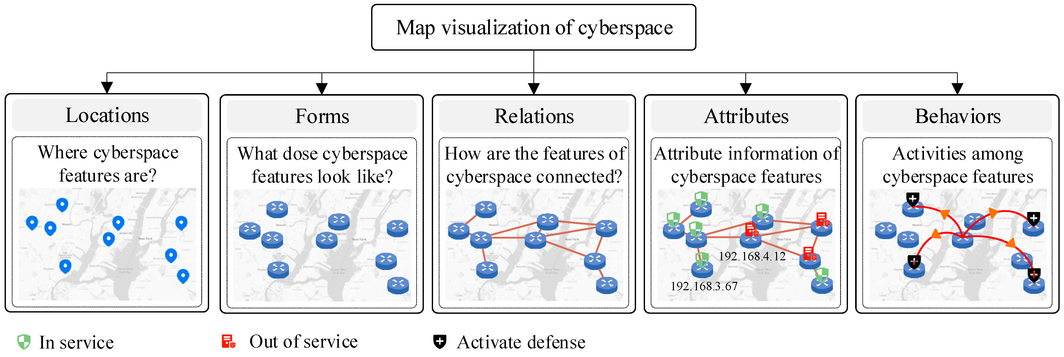
The content represented in CMV differs from that of traditional maps. While traditional maps primarily depict the spatial and attribute characteristics of geographic features, cyberspace maps must also represent information such as relationships, behaviors, and forms of cyberspace features. Based on an analysis and summary of existing cyberspace maps, this study categorizes the main representation content into five aspects, namely locations, forms, relations, attributes, and behaviors, as shown in Figure 1.

Figure 1.
Main representation content of CMV.
Among them, “locations” refers to the positioning of cyberspace features, mainly answering the question, “Where are cyberspace features distributed?” In general, these features can be mapped to physical locations in the real world [36]. For example, the geographic coordinates of an IP address can be determined through IP geolocation technology. “Forms” refers to the morphological characteristics and manifestations of cyberspace features, mainly addressing the question, “What do cyberspace features look like?” For example, different symbols are often used to represent different types and statuses of cyberspace features. “Relations” mainly answers the question, “How are cyberspace features related?” This aspect is crucial in differentiating CMV from traditional map visualization. Cyberspace features often have complex relationships, such as connectivity and membership relationships. “Attributes” refers to the nonspatial information of cyberspace features, such as IP addresses, device information, status information, and statistical information. “Behaviors” refers to the interactive activities between cyberspace features, such as DDoS cyberattacks and network communication behavior.
2.3. Symbol System
The symbol system forms the foundation and core of CMV. Compared with symbol systems in ordinary maps, the symbols used in cyberspace maps differ in terms of representation accuracy, methods, and objects. However, they should still build upon and extend the principles and concepts from traditional map symbol design. Therefore, the design process for cyberspace map symbols should adhere to relevant principles, methods, and concepts in traditional map symbol design [37].
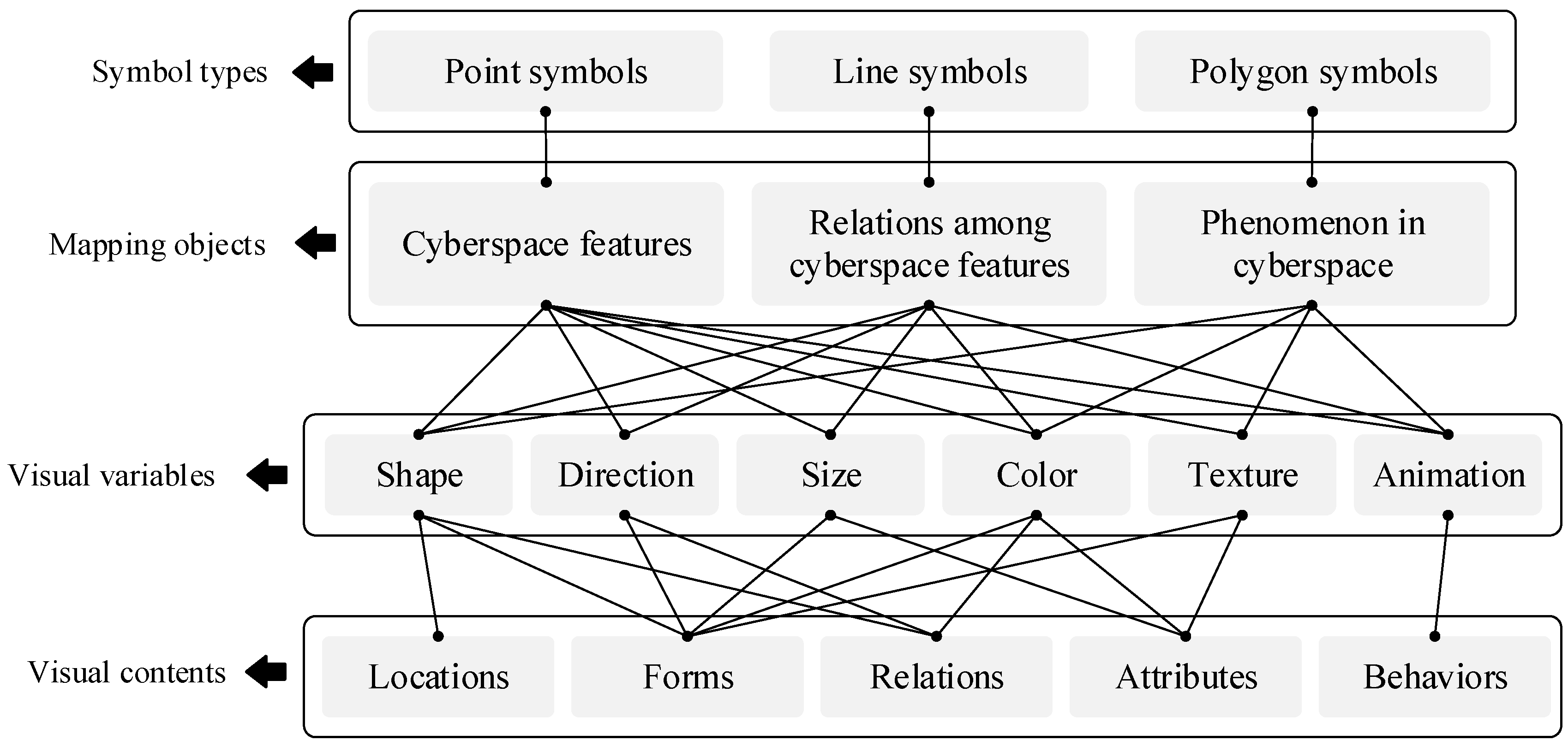
The symbol system for CMV is shown in Figure 2. The objects represented by this symbol system can be mainly divided into cyberspace features, relationships (including behaviors) between cyberspace features, and various phenomena in cyberspace (such as statistical information and scope of services). Corresponding to these objects, the symbol types in CMV include point, line, and polygon symbols.

Figure 2.
Symbol system of CMV.
- Point symbols.
Point symbols in cyberspace maps are mainly used to represent cyberspace features, such as network devices, virtual accounts, software systems, and communication base stations. These symbols use visual variables such as shape, direction, size, color, animation, and texture to represent information such as the spatial location, spatial form, and attribute characteristics of features.
- 2.
- Line symbols.
Line symbols in cyberspace maps are mainly used to represent the relationships or behaviors between cyberspace features, such as the connections between network devices, communications between these devices, and cyberattack activities between servers. Linear symbols use visual variables such as shape, direction, color, animation, and size to represent the relations and behaviors between features.
- 3.
- Polygon symbols.
Polygon symbols in cyberspace maps are mainly used to represent various phenomena in cyberspace features, such as the service area and distribution density of network devices. It should be noted that CMV is mainly based on point and line symbols, and polygon symbols are used only in a few cases (such as statistical thematic maps and cartogram maps).
3. Data Model for CMV
Data models have been a research hotspot in the field of geographic information science. They define how geospatial features or phenomena are represented and stored conceptually, logical, and physically, thus supporting applications such as analysis and visualization [38]. However, existing geospatial data models fail to directly support the representation of cyberspace features and their relations. Therefore, it is necessary to design appropriate data models to meet the application needs of CMV.
3.1. Conceptual Model
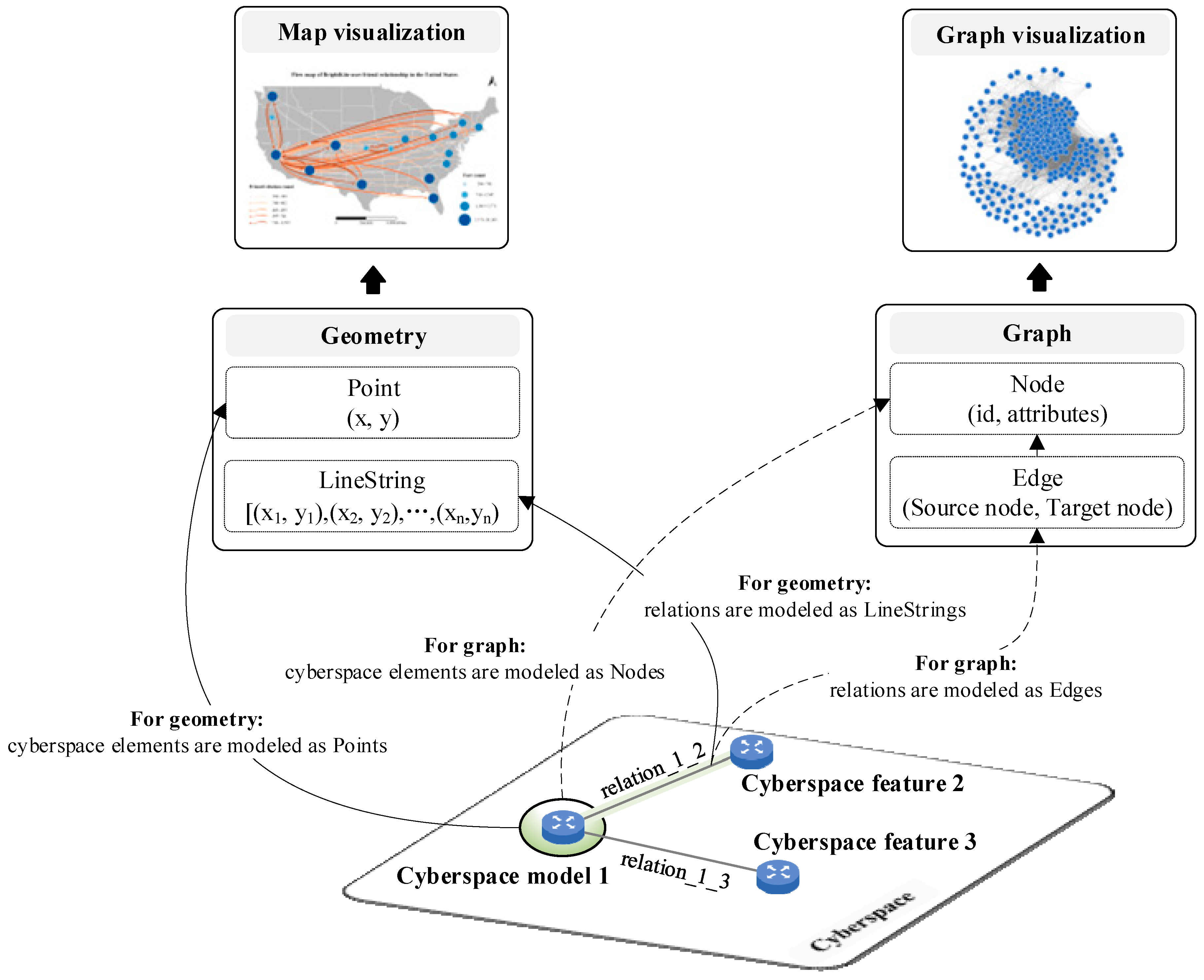
A conceptual model is “a mathematical/logical/verbal representation (mimic) of a domain (real or proposed), situation, policy, or phenomenon developed for a particular study” [39]. To better understand the data model for CMV, a conceptual model for CMV is designed in this study, as shown in Figure 3.

Figure 3.
Conceptual model for CMV.
To facilitate map visualization, this paper models the elements and their relationships in cyberspace as geometric points (Point) and line strings (LineString). Specifically, the coordinate positions of cyberspace elements are mapped to the x and y values of points, while the relationships between elements are represented by line segments connecting the start and end points. However, this geometry-based modeling approach is primarily intended for visualization and does not support complex network queries, analyses, or visual layouts, as it lacks reference relationships between geometric entities.
To address this issue, this paper not only models the elements of cyberspace as geometric shapes but also further represents them as nodes (Node) and edges (Edge) in a graph model (Graph), where each edge is defined by a starting node and an ending node. By introducing a “geometry-graph” composite data model, this paper can simultaneously support efficient map visualization and complex network analysis.
3.2. Logical Model
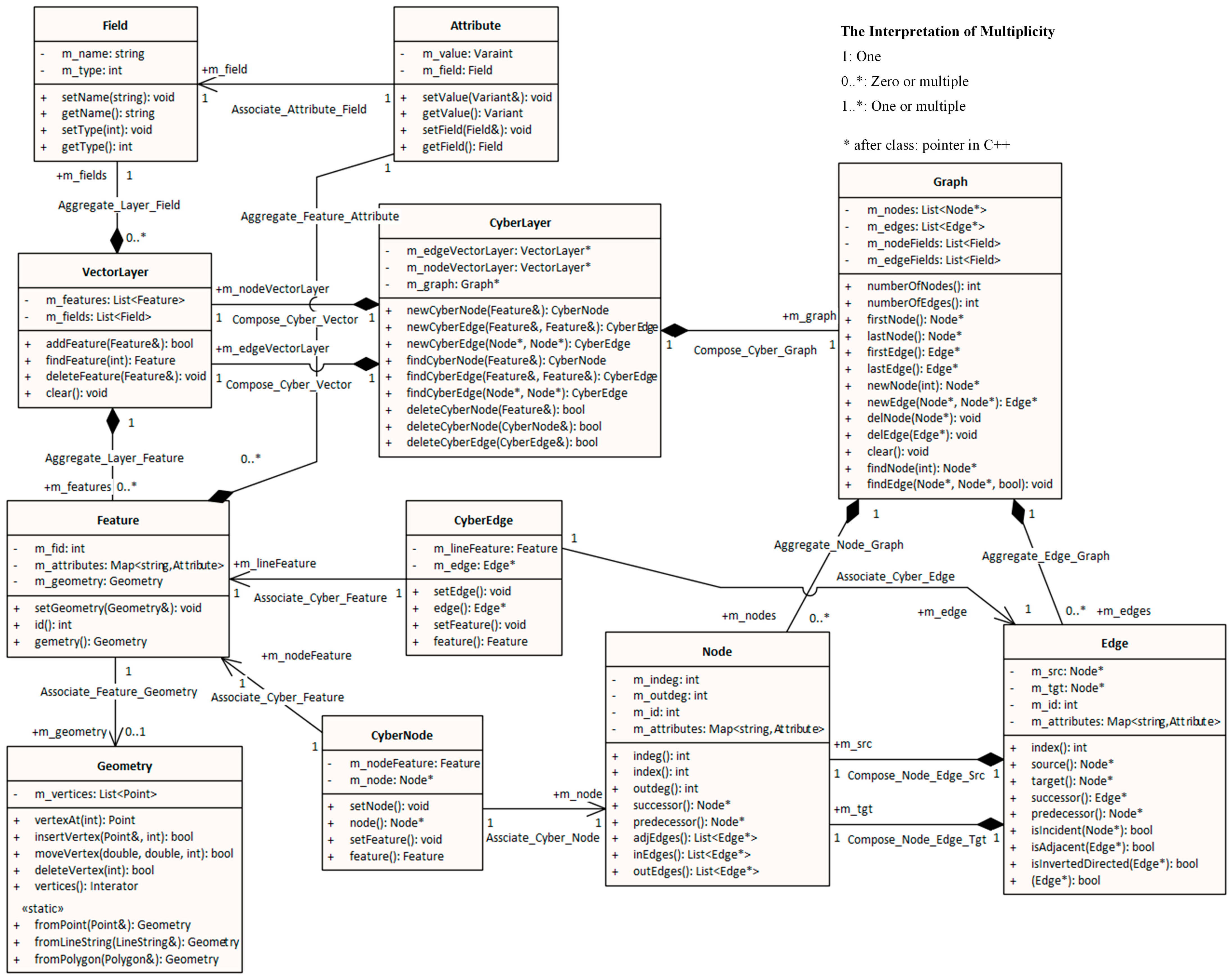
According to the design philosophy of the conceptual model, we design a logical model of CMV and draw a UML class diagram, as shown in Figure 4. CyberLayer is a cyberspace layer class, which contains two VectorLayer classes and one Graph class. The VectorLayer classes correspond to the point vector layer and the line vector layer, which are used to represent cyberspace features and the relationships (or behaviors) between features. The VectorLayer class is consistent with the spatial data model of ordinary GIS, aggregating spatial features, with each feature containing geometries. The graph, which is composed of nodes and edges, is a typical graph (network) structure model that is mainly used to maintain the relations between the features of the point vector layer and the line vector layer, providing an efficient query interface to quickly retrieve nodes or edges.

Figure 4.
UML class diagram of the data model.
The logical model described above essentially adopts a “proxy mode”, providing a unified interface to manage spatial and cyber features by capturing the spatial and graph models. The advantage of this model is that it can support both map visualization and complex network queries, analysis, and visualization layouts, and it does not require additional code to maintain data consistency between the spatial data model and the graph model.
3.3. Physical Model
Based on the logical model, we design a physical model for CMV. This model is mainly used for the instances of relational databases. It should be noted that, as graph database technology matures and is increasingly applied, the physical model can also be designed according to the graph database paradigm [40]. Owing to the simplicity of the methods involved in this part, we do not discuss them in this paper.
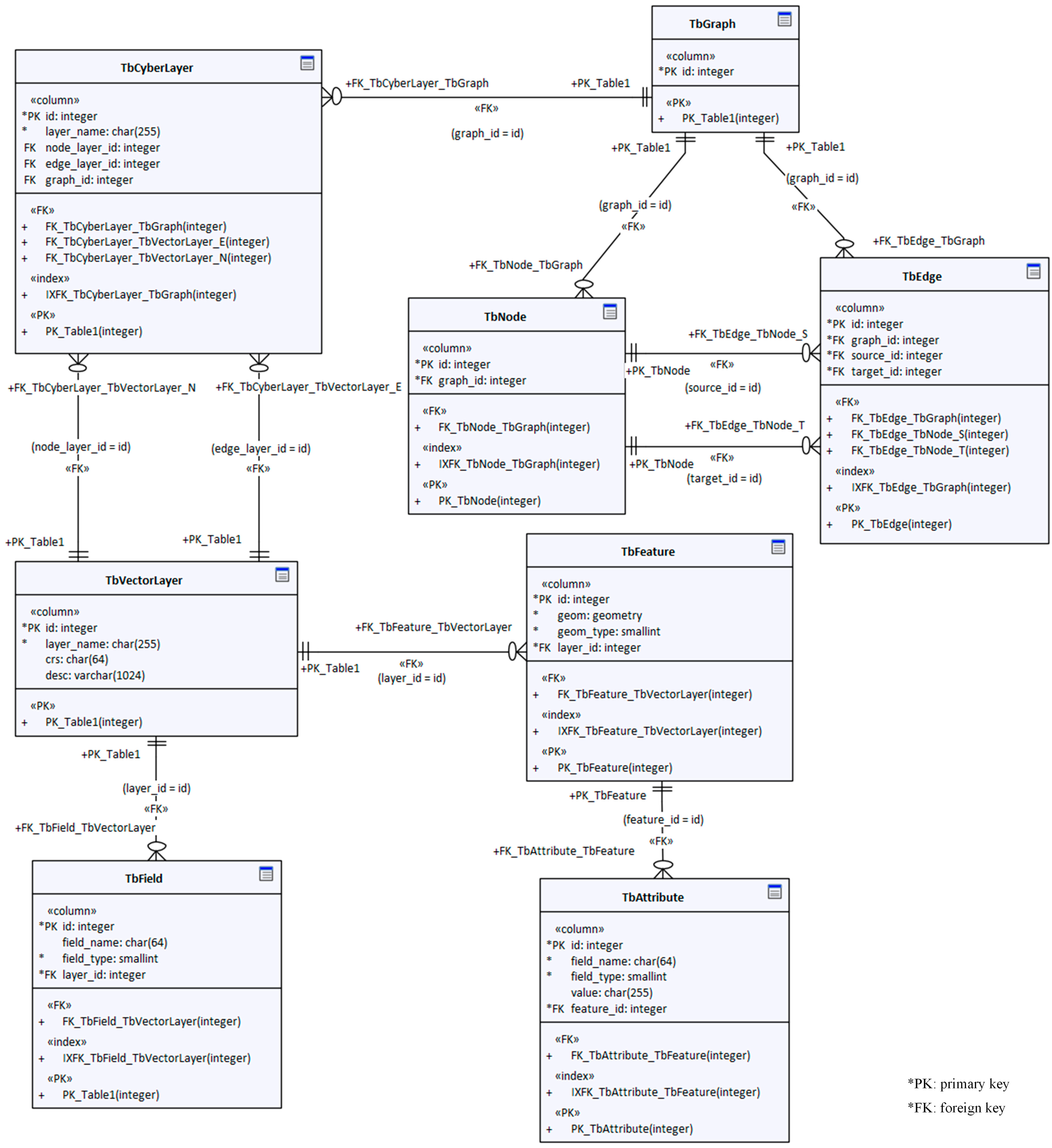
To facilitate comparison with the logical model, we add the prefix “Tb” to each database table of the physical model, as shown in Figure 5. In this way, the naming of the physical model is essentially aligned with that of the logical model on a one-to-one basis. For relational databases, the combination, aggregation, and relations in the logical model are implemented mainly through the “foreign keys” in the database tables of the physical model.
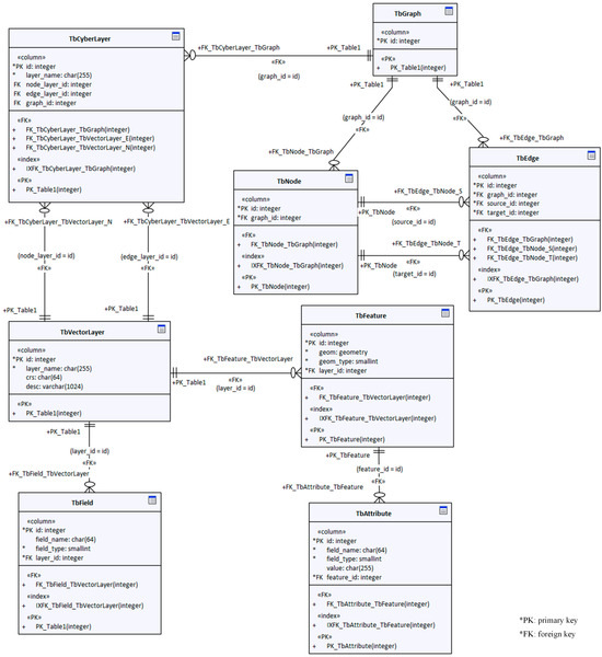
Figure 5.
Table structure design of the relational database of the data model.
Unlike the logical model, the physical model does not need a separate table for geometry information. Because most database products now directly support geometry fields, we incorporate geometry as a field in the vector layer database table (TbVectorLayer).
4. Method Framework for CMV
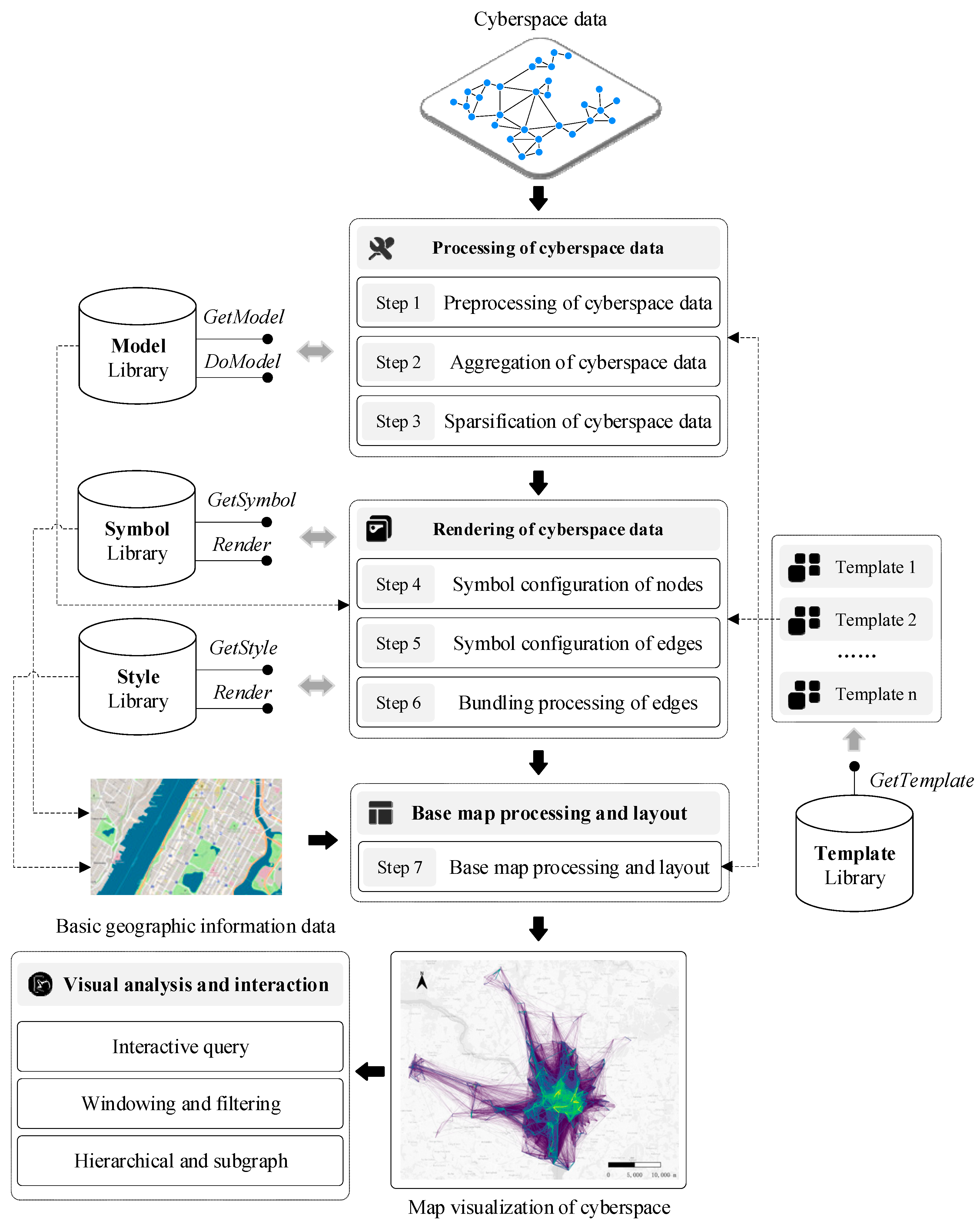
CMV essentially falls under the category of thematic map visualization. Therefore, its visualization method also follows the general process of thematic visualization—that is, thematic layer processing, base map layer processing, and map layout. Based on the above concept, we design a method framework for CMV, as shown in Figure 6. This framework includes three main stages (seven key steps): cyberspace data processing, cyberspace data rendering, base map processing and map layout. Each stage is completed with the support of the corresponding libraries, including the model, symbol, style, and template libraries.
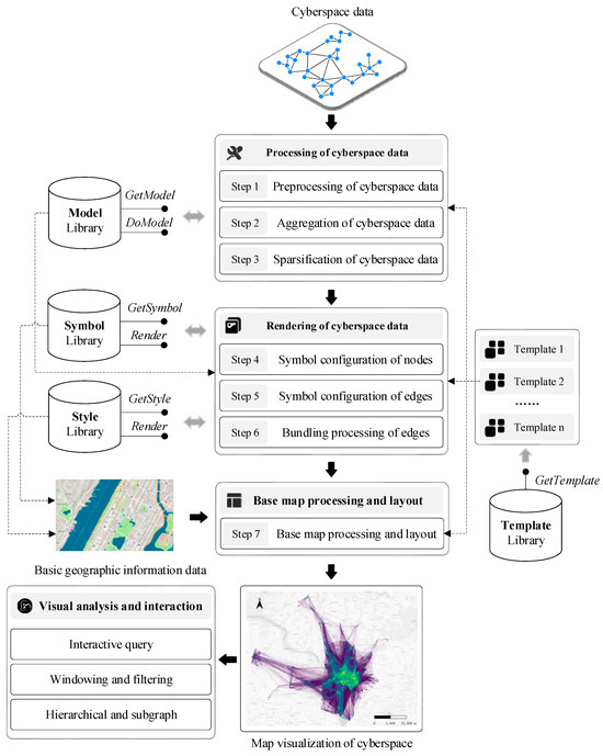
Figure 6.
Method framework for CMV.
4.1. Cyberspace Data Processing
Due to the different standards and large volume of cyberspace data, the data need to be processed during CMV, including operations such as data preprocessing, data aggregation, and data sparsification.
4.1.1. Data Preprocessing
For cyberspace data, data preprocessing involves format conversion, coordinate transformation, and data cleaning. This process is carried out with the support of the model library. There are various cyberspace data standards and formats, the most common of which are CSV [41], GEXF [42], GML [43], and GraphGML [44]. Therefore, it is necessary to load these data using custom-written code or plug-ins and convert them to the data model of the corresponding system. Currently, the spatial coordinates of the most cyberspace data adopt geographic coordinate systems such as WGS84. However, when performing CMV, the geographic coordinates need to be converted to projected coordinates—a process that is consistent with ordinary thematic map visualization. Cyberspace data are acquired from various sources and involve complex acquisition technologies, which, as a result, may lead to noise, errors, omissions, and redundancy in the data. Therefore, it is necessary to perform cleaning on cyberspace data through smoothing, modification, imputation, and deletion.
4.1.2. Data Aggregation
Cyberspace data aggregation is the process of merging spatially adjacent nodes and edges. This process is mainly carried out with the support of the model library. Cyberspace data aggregation is not a necessary step for visualization. Data aggregation is typically needed for two reasons. First, the inaccuracy of data collection causes nodes that should have been merged to remain unmerged; second, due to actual application requirements, nodes need to be merged according to certain statistical units.
The cyberspace data aggregation process is as follows. First, nodes are divided into different sets through spatial clustering units and spatial statistical areas. Then, the spatial coordinates , in-degree , and out-degree of a aggregated node are calculated. For each set, denotes the coordinates of the aggregated node, serving as the geometric centroid of all nodes within the aggregation set. denotes the number of nodes in the set. denotes the longitude of node within the aggregation set, while denotes the latitude of node within the set. Considering the spatial positioning errors of nodes in cyberspace, uncertainty must be accounted for when calculating . Let and denote the widths of the confidence intervals in the X and Y directions, respectively. denotes the in-degree of the aggregated node and equals the count of edges whose terminal nodes are within the set. denotes the out-degree of the aggregated node and equals the count of edges whose original nodes are within the set. denotes the overall degree of the aggregated node. The specific calculation formulas are as follows:
Second, to reflect the results of information aggregation, the weights of the edges need to be processed and calculated. Suppose each edge possesses computable attributes, with each attribute associated with a distinct weight value . Let denote the th attribute value of edge ; consequently, the weighted attribute of this edge can be computed. For two aggregated sets and , let denote the number of edges where the starting node is within set and the ending node is within set . Then, the edge attribute value of two aggregated sets is equal to the sum of all edge attribute values between these sets. The calculation formulas are as follows:
Based on Formula (2), the edge attribute values V between all pairs of aggregated sets can be computed. Following the normalization of these attribute values, the weight of the aggregated edges are derived, as presented in the formula:
For large-scale cyberspace data, aggregation processing can be time-consuming, primarily due to the high computational complexity involved in spatial calculations during node aggregation. To enhance computational efficiency, the study area can be partitioned into grids, transforming the distance calculations between nodes into those between grid cells, thereby significantly improving the efficiency of aggregation processing.
4.1.3. Data Sparsification
The number of edges in cyberspace data grows exponentially with the increasing number of nodes, leading to a massive data scale, and direct visualization often causes severe visual clutter. Cyberspace data sparsification is the process of deleting or filtering out less important structures based on the importance indicators of nodes or edges to compress the size of cyberspace data and improve the signal-to-noise ratio of the data. This process is carried out with the support of the model library. In general, there are two main methods for cyberspace data sparsification. The first method involves ranking and selecting nodes based on their importance or attributes, such as degree centrality [45], betweenness centrality [46], closeness centrality [47], or eigenvector centrality [48]. The other method involves ranking and selecting edges based on their weights or attributes. The first method is significantly less efficient than the second method due to the requirement of calculating node centrality. Consequently, for large-scale cyberspace data, it is recommended to adopt the second method for the efficiency of sparsification.
Data reduction and data aggregation are both forms of data generalization. However, data sparsification removes part of the structure, equivalent to selection in cartographic generalization, whereas data aggregation combines information, equivalent to merging in cartographic generalization.
4.2. Cyberspace Data Rendering
Cyberspace data consist of features and the relationships between them, serving as the carrier of information stored in computers. Only when these data are mapped into specific symbols can they be recognized by humans—a process known as cyberspace data rendering.
4.2.1. Node Symbol Configuration
Node symbols in cyberspace data translate spatial coordinates into symbols with specific positional information through graphics and images. These symbols represent information such as the type, mass, quantity, and status of cyberspace nodes by adjusting visual variables such as the shape, color, orientation, and size of the symbols. This process is supported by the symbol and style libraries. In general, node symbols use point-located symbols, such as geometry symbols, text symbols, or pictorial symbols, with circle or square outlines added to the outside of the symbols to highlight the target.
The visual variables of node symbols can be related to mathematical models, allowing for the classification of nodes according to cyberspace feature attributes. This process requires the support of the model library. For example, the size of a node can be classified according to the attribute field’s values using equal-interval or proportional classification.
4.2.2. Edge Symbol Configuration
The edges of cyberspace data use linear symbols to represent the relationships and activities between cyberspace features. The mass, quantity, and orientation of (and other information about) the edges in cyberspace are represented by adjusting visual variables such as the color and size of the symbols. This process is supported by the symbol and style libraries. The direction of the edges is generally represented by linear symbols with arrows. However, when the scale of cyberspace data is large, the intertwined edges make it difficult to distinguish the direction of the arrows. In this case, a gradient color from the start to the end of the edge is often used to indicate the direction.
Similar to node symbols, the visual variables of edge symbols can also be associated with mathematical models, allowing them to reflect a classification effect based on the weights or attribute values of the edges.
4.2.3. Edge Bundling
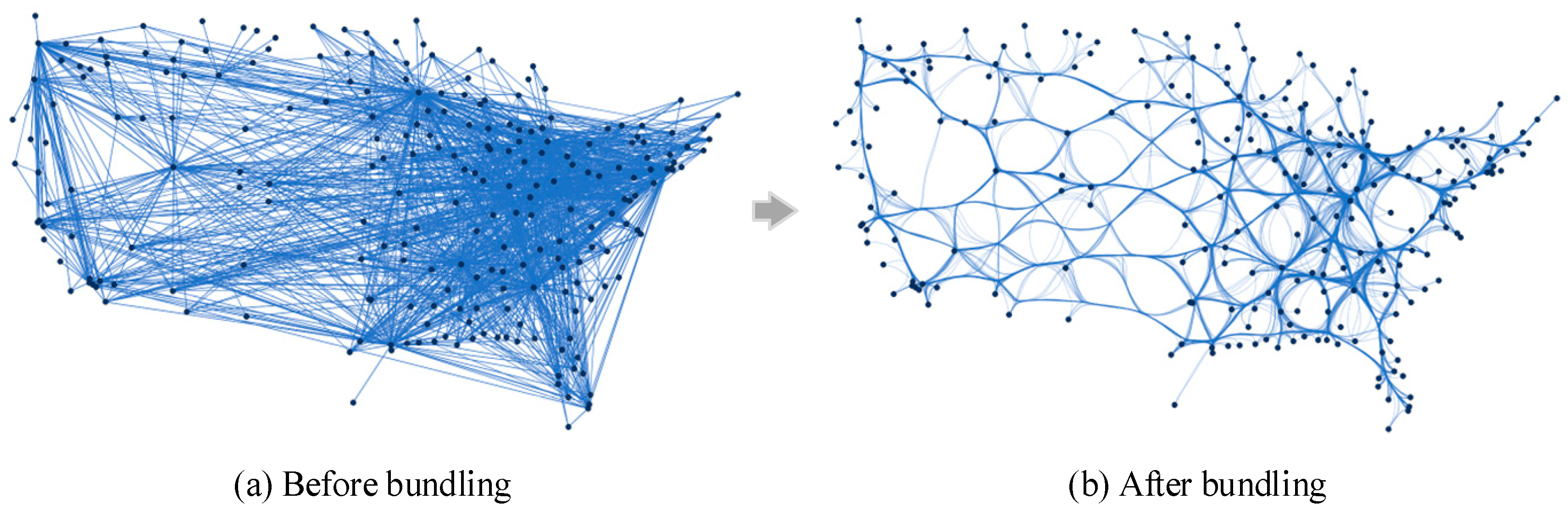
When dealing with large-scale cyberspace data, in addition to using data aggregation and data sparsification methods for processing, edge bundling can be used to reduce the visual load of edges from the perspective of visualization. In network edge bundling, the path of the edges is replanned, and the edges with a similar direction, distance, and length are bundled together to highlight the higher-order skeleton structure of the network and reduce the visual clutter caused by intertwined edges, as shown in Figure 7. This process is supported by the model library.
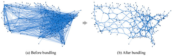
Figure 7.
Edge bundling.
Let be the visualization space of edge and be the visualization space after edge has been bundled. is the bundling processing for the edge when the following conditions are satisfied:
where is the distance between edges, such as the Hausdorff distance [49] is the compatibility index between edges, which is generally calculated based on the distance, direction, and length between edges. Common-edge bundling algorithms include FDEB [26] and KDEEB [28]. The FDEB algorithm, which requires the iterative computation of edge compatibility, often demonstrates lower efficiency compared to the KDEEB algorithm when processing large-scale cyberspace data. Therefore, this paper primarily employs the KDEEB algorithm for handling large-scale datasets. Figure 7 shows the result of KDEEB edge bundling.
4.3. Base Map Processing and Layout
The primary goal of CMV is to represent the distribution of cyberspace features, along with their relationships and activities, using basic geographic information as the base map for visualization. During base map processing, such as feature selection and symbol rendering, efforts should be made to ensure the clarity and prominence of the representation of the cyberspace thematic layer. In general, the number of base map features should not be too large, and the number of linear features should be minimized to avoid confusion with the edges in the cyberspace thematic layer. In terms of coloring, the base map layer should choose a color system with strong contrast to the cyberspace thematic layer. For example, if the cyberspace layer uses dark colors, the base map layer should choose light colors to highlight cyberspace thematic features.
Unlike conventional thematic map visualization, relevant cartographic norms and standards have not yet been developed in the field of CMV, resulting in different styles of symbol configuration and map coloring. Therefore, auxiliary map reading features such as map titles, legends, insets, and text descriptions become particularly critical. The CMV layout process involves determining the locations of these features through reasonable spatial configuration.
4.4. Visual Analysis and Interaction
Cyberspace data have a rather complex association structure. Interactive visualization methods can help users better understand and analyze the data. Common interactive visualization methods for cyberspace data include interactive query, windowing and filtering, and hierarchical and subgraph methods.
Interactive query is a foundational method for exploring cyberspace data. It allows users to interactively select or query elements, such as highlighting edges connected to a selected node or visualizing the connectivity path between two nodes.
Windowing and filtering visualization is a method for analyzing cyberspace data by defining a localized view. It enables the selection or arrangement of nodes and edges within the defined window based on specified filtering criteria, facilitating interactive analysis of network data in regions of interest.
Hierarchical and subgraph visualization is a method for organizing and visualizing cyberspace data in layers based on their types. This approach is primarily used to investigate the relationships between cyberspace data across different hierarchical levels. Each layer represents a subgraph of the network, allowing for independent layout and analysis of the cyberspace data within that layer.
5. CVM Experiments and Discussion
To validate the rationality and feasibility of the proposed data model and method framework, we designed and implemented a web-based system for CMV and conducted several map visualization experiments using the “Routers and router relationships dataset of northern Taiwan” (Routers), “BrightKite dataset of United States” (BrightKite), and “Global submarine optical fiber cables dataset” (Cables).
5.1. CMV System
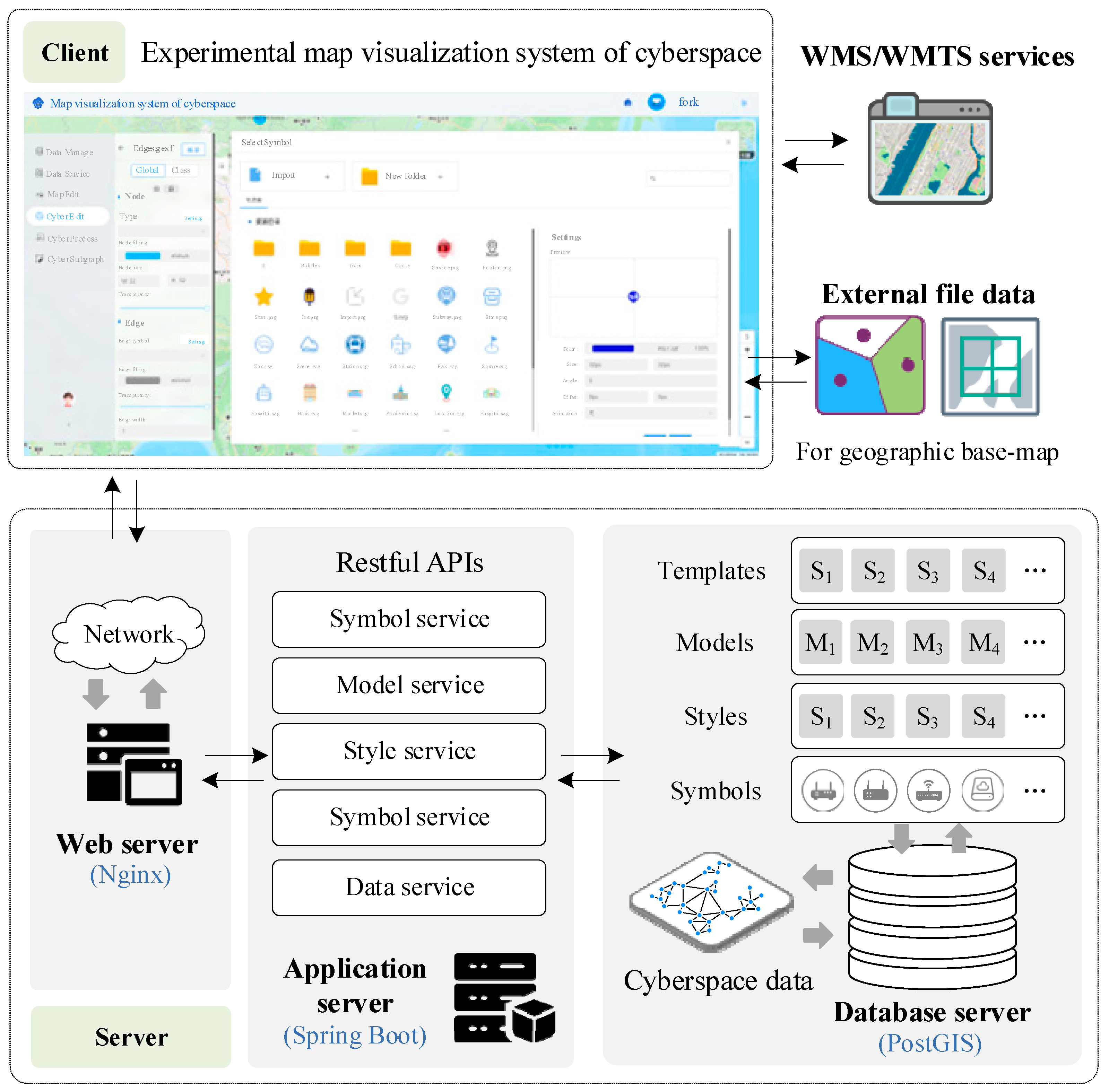
The CMV system employs a B/S architecture, as shown in Figure 8. Nginx serves as the web server to handle the HTTP requests from clients, organize the request parameters into JSON format data, and forward them to the application server. The application server utilizes Spring Boot as the application service framework to provide symbol, model, style, and data services in the form of microservices. PostGIS is used as the database server to store and manage cyberspace data, geospatial data, and related business data.

Figure 8.
Architecture of the CMV system.
The system provides functions such as data management, data editing, symbol rendering, and map layout. For the basic geographic base map, the user can access third-party WMS/WMTS services or upload and load vector or raster file data. The system performs the map visualization of cyberspace data on the frontend and renders and exports the completed map on the server side.
5.2. Experimental Data and Processing
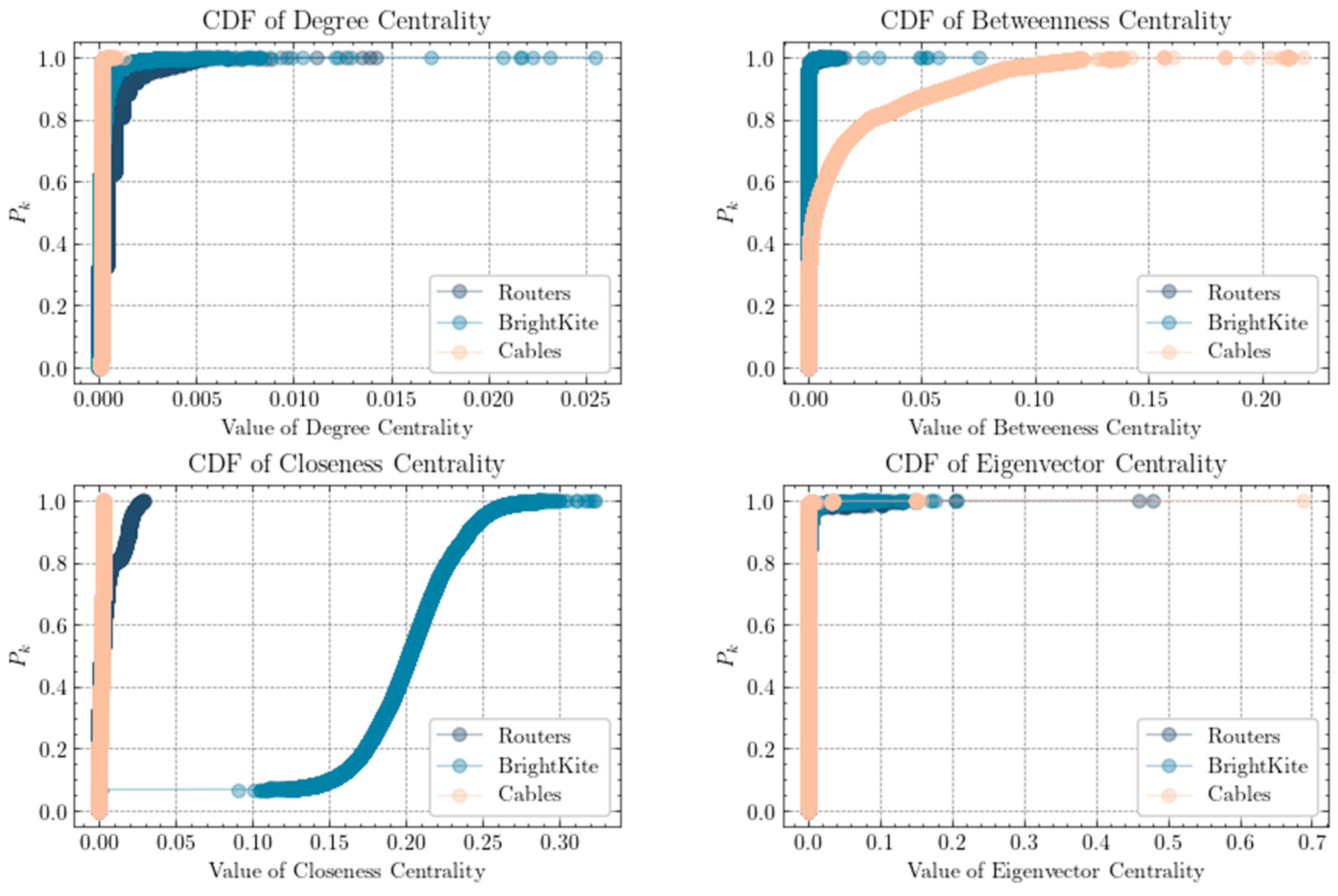
To better comprehend the fundamental characteristics of the data, we conducted a comprehensive statistical analysis encompassing the number of nodes, the number of edges, degree centrality, betweenness centrality, closeness centrality, and eigenvector centrality. Additionally, we generated CDF curves for these centrality measures, as detailed in Table 1 and illustrated in Figure 9.

Table 1.
Statistical Summary of the Experimental Datasets.

Figure 9.
CDF curves of centrality metrics in the experimental dataset.
- The Router Dataset and Its Processing.
The data used in the experiment consist of router relationship data from northern Taiwan, covering Taipei City, New Taipei City, Keelung City, Taoyuan City, Hsinchu County, Hsinchu City, the Matsu area, and Yilan County. The BNF normal form for router dataset entries is described as follows:
where is the unique identifier of the router, are the unique identifier and name of the AS autonomous domain, respectively, and represent router roles (such as core router, area router, and intermediate router), and are the spatial position coordinates of the router. The BNF normal form of relational dataset entries is described as follows:
where is the unique identifier of the higher-level router and represents the AS autonomous domain where the topological relationship is located. When constructing the relationships between routers, we set as the source node and use as the target node.
As shown in Figure 9 the shape of the CDF curves indicates that they are essentially logarithmic functions. In this type of network, most nodes are not connected to each other, but from any given node, other nodes can be accessed through a certain step size or hop count. This result shows that the router relationship network exhibits typical small-world network characteristics.
If the original router relationship data are directly used for map visualization, the large numbers of nodes and edges can lead to cluttered visualization and poor legibility. To address this, based on the small-world network characteristics, less important nodes can be filtered out—that is, data sparsification is conducted, while maintaining the spatial distribution characteristics of the overall network. Figure 10 shows the results of cyberspace data sparsification at different compression ratios. We use the result with a compression ratio of 60% as an example to conduct the subsequent CMV experiment.
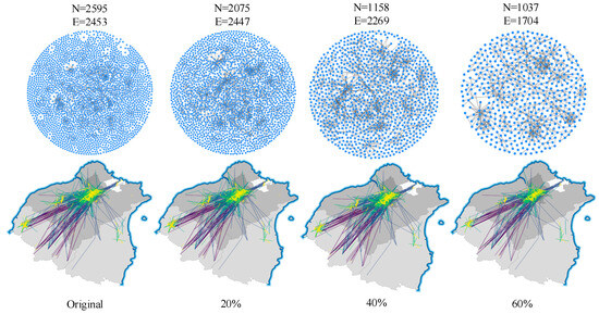
Figure 10.
Cyberspace data sparsification.
- 2.
- The BrightKite Dataset and Its Processing.
The BrightKite dataset encompasses check-in location data within the United States, sourced from the publicly available LBSN dataset (http://snap.stanford.edu/data/loc-brightkite.html (accessed on 12 December 2024)). It comprises both social network information and check-in records. To more accurately represent users’ places of residence, this study adopts the centroid of all check-in locations for each user as their place of residence [50]. Based on this approach, the network structure of the BrightKite dataset was constructed. The BNF notation for this dataset is described as follows:
where denotes the unique identifier of the user, denotes the longitude of the user’s place of residence, and denotes the latitude of the user’s place of residence. The BNF normal form for the entries in the relational dataset is described as follows:
where and respectively denote the user identifiers of two users with a friend relationship.
As shown in Table 1, the BrightKite dataset is significantly larger than the Router dataset. Even after compression, it remains challenging to clearly visualize the BrightKite dataset using a node-link map. To address this issue, this paper aggregated the BrightKite dataset at the state level of the United States as the basic statistical unit. Specifically, each state was treated as a node, and virtual friend relationships between states were represented as edges. Edge weights were determined by counting the number of friendships between users in different states. Finally, a flow map visualization experiment was conducted using the aggregated network data. Following the data processing, the initial network comprising 29,393 nodes was consolidated into 49 representative nodes. Additionally, the original 196,926 edges were reduced to 58 significant connections, with edges representing fewer than 300 friendships being excluded from the aggregation process.
- 3.
- The Cables Dataset and Its Processing.
The Cables dataset encompasses global submarine optical cables and their associated landing station. In this paper, landing stations are treated as nodes, and the optical cable lines connecting pairs of landing stations are represented as edges to construct the network-structured Cables dataset. The BNF normal form description is as follows:
where denotes the unique identifier of the landing station, denotes the name of the landing station, denotes the longitude of its location, denotes the latitude of its location, and denotes the country to which the landing station belongs. By treating direct optical cable connections between two landing stations as edges, the association relationship data between landing stations can be constructed. The BNF normal form description is as follows:
where and denote the unique identifiers of two landing stations directly connected by submarine optical cables, denotes the power of the optical cable, denotes the length of the optical cable between the two landing stations, and indicates whether the optical cable line remains in service.
For the Cables dataset, the positions of landing stations and optical cables are fixed and cannot be altered arbitrarily. Therefore, a feature distribution map can be employed to accurately depict the spatial distribution of landing stations and optical cables.
5.3. CMV Experiment
Using the CMV system and the experimental datasets, we generated the following types of cyberspace maps: a statistical thematic map of router roles, a node-link map of router distribution, a bundling map of high-level router distribution, a flow map of BrightKite user friend relationship in the United States, and a feature distribution map of global submarine fiber cables.
- Statistical thematic map of router roles in northern Taiwan.
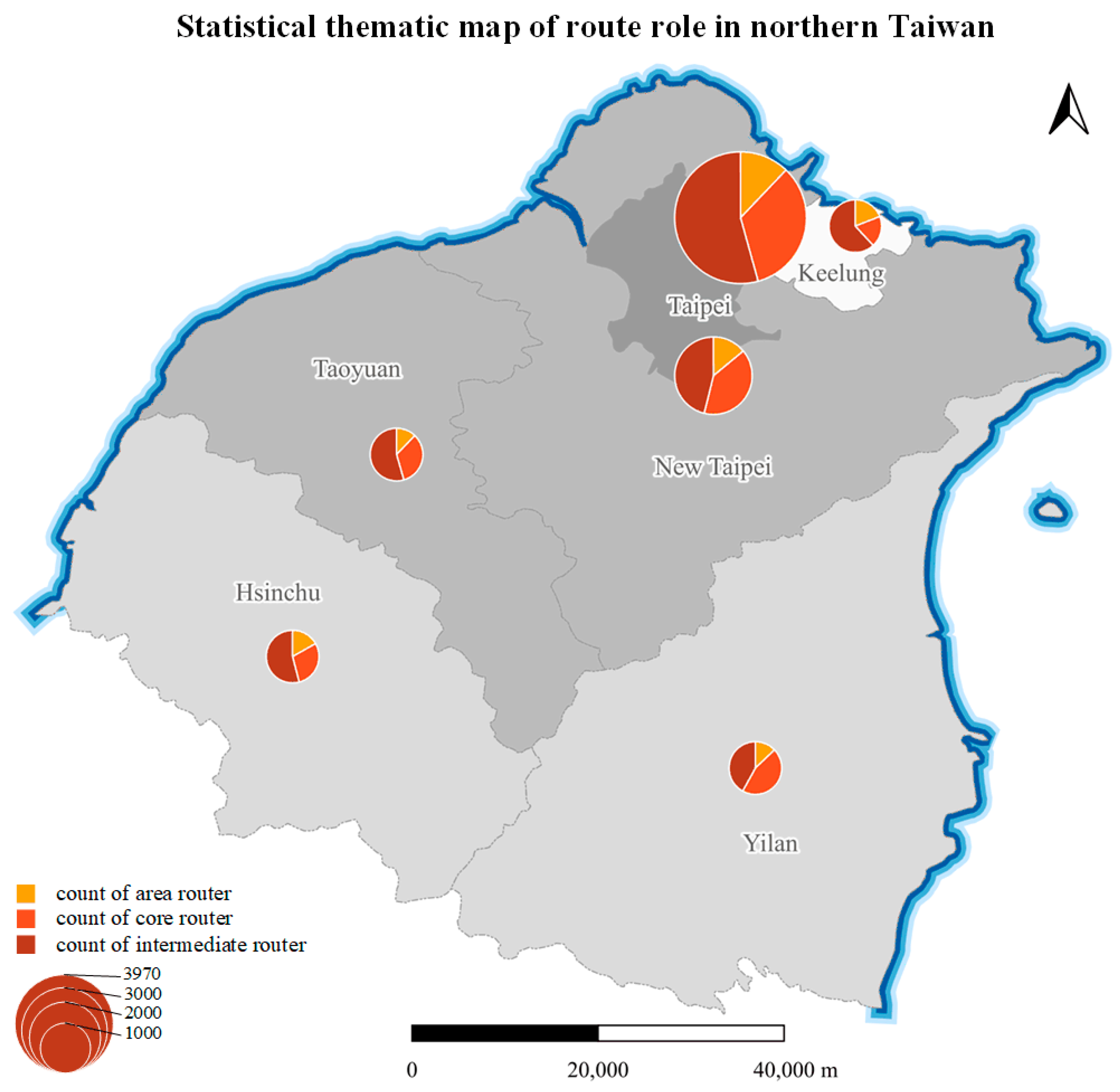
Using the municipal divisions of northern Taiwan as units, we calculated the numbers of area, core, and intermediate routers within each unit and constructed a statistical thematic map of router roles in northern Taiwan using pie charts, as shown in Figure 11.

Figure 11.
Statistical thematic map of router roles in northern Taiwan.
Taipei City has the largest number of routers, followed by New Taipei City, with other cities and counties having relatively fewer routers, reflecting the level of network informatization in various cities and counties in northern Taiwan. In each city or county, the number of intermediate routers is the largest, followed by that of core routers, and the number of area routers is the smallest, which is also closely related to the functions of different routers. For example, intermediate routers mainly serve to expand network coverage, alleviate router pressure, and improve signal quality. Therefore, intermediate routers have the highest proportion in each city or county. However, Yilan County and New Taipei City have a relatively low proportions of intermediate routers compared to those of other cities and counties, which may be related to their topography and population distribution. For example, south of Yilan County is mountainous, with the population concentrated in its northern part, limiting the distribution area. As a result, the required network coverage is smaller, leading to fewer intermediate routers.
- 2.
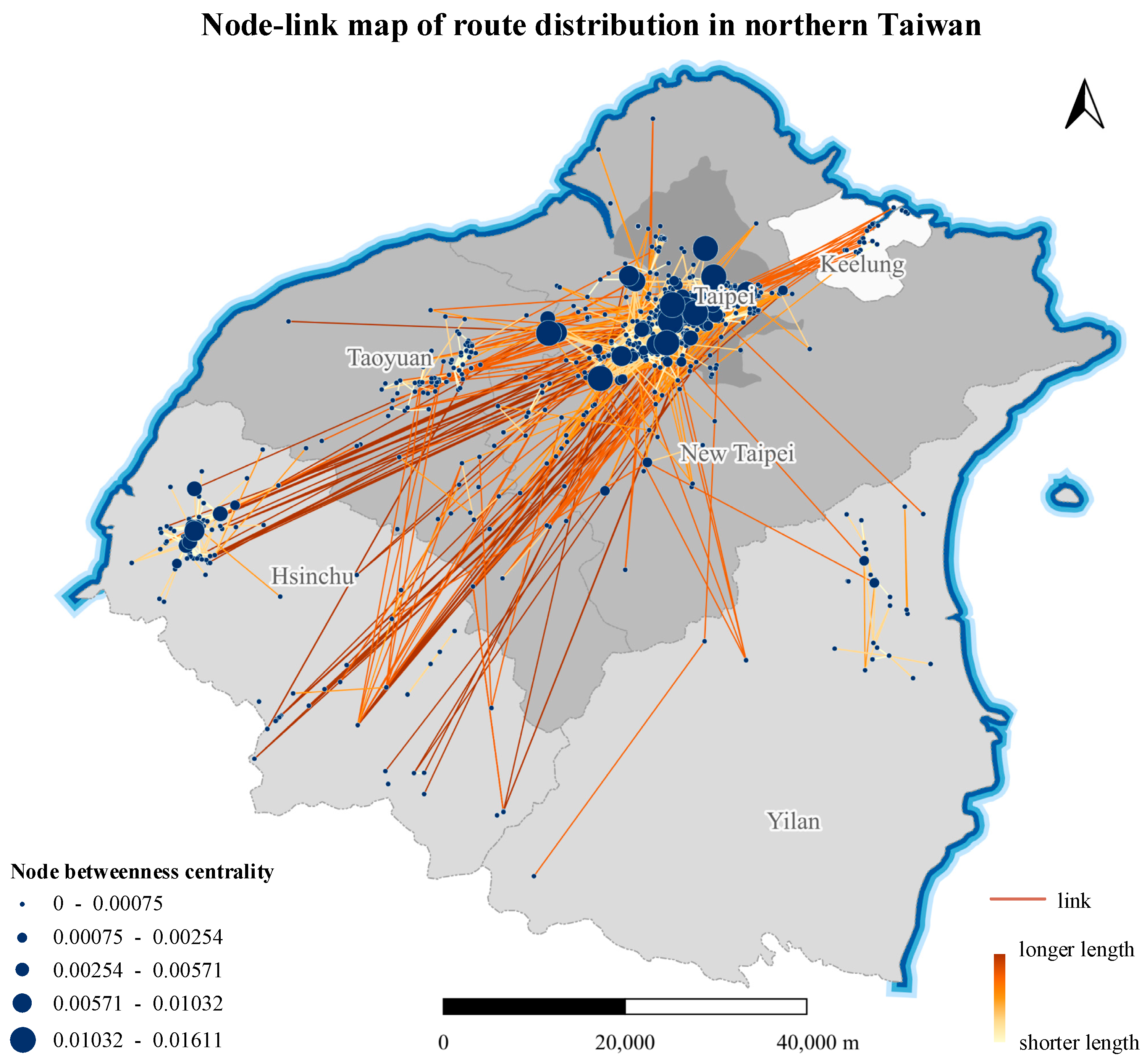
- Node-link map of router distribution in northern Taiwan.
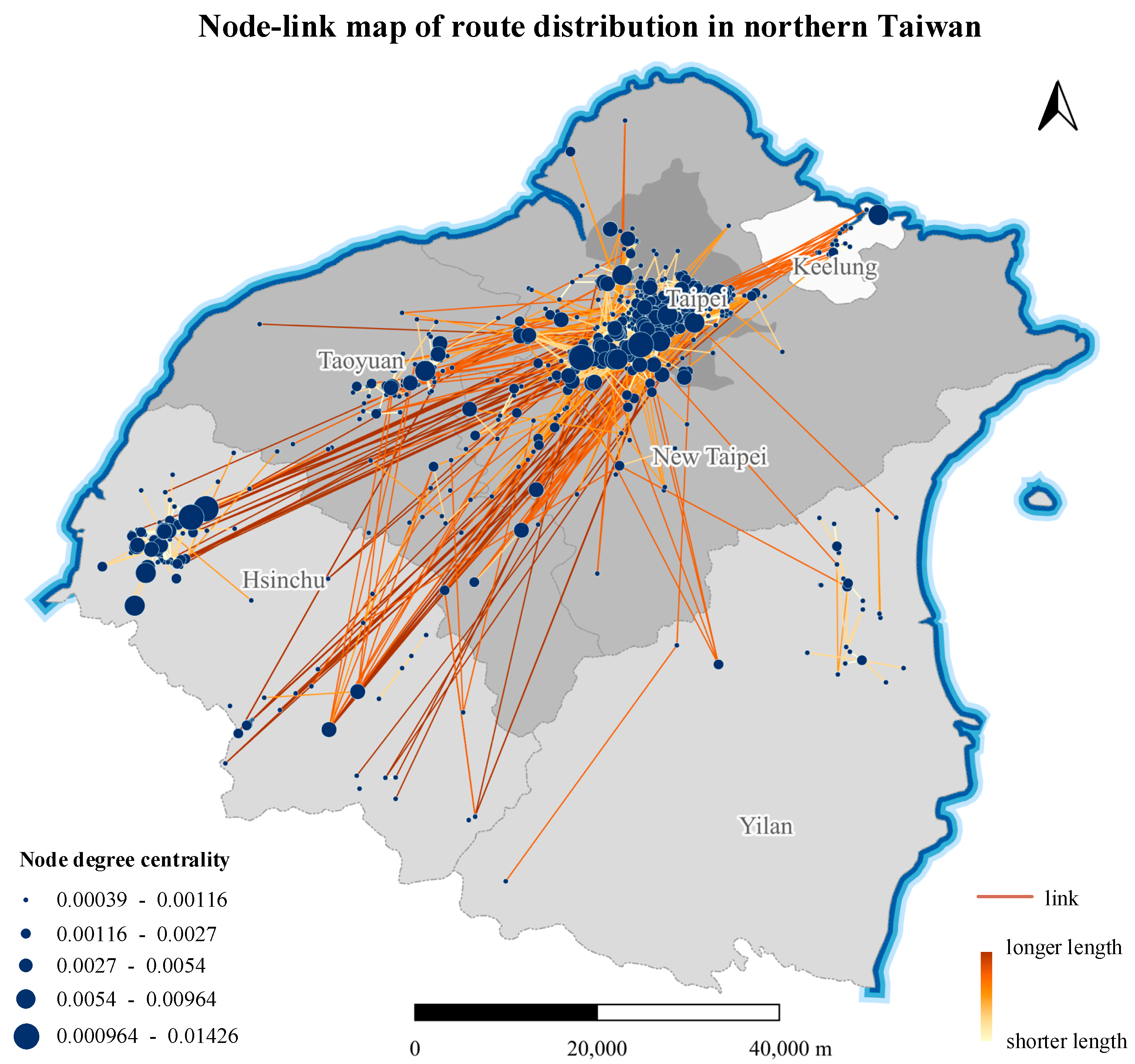
The degree centrality and betweenness centrality of each router in the network were calculated, and node-link maps of router distribution in northern Taiwan were plotted using the two centrality values as a classification basis, as shown in Figure 12 and Figure 13, respectively.
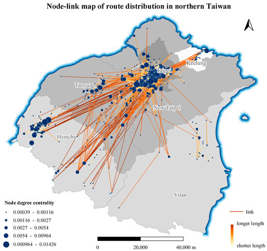
Figure 12.
Node-link map of router distribution in northern Taiwan (degree centrality).
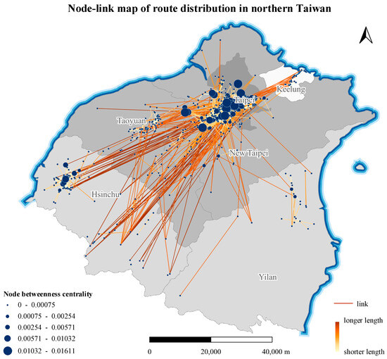
Figure 13.
Node-link map of router distribution in northern Taiwan (betweenness centrality).
A higher degree centrality means that a router is directly connected to a greater number of other routers. Figure 12 shows that Taipei City has the most routers with high degree centrality, followed by Hsinchu City and Taoyuan City. This result indicates that other cities and counties have close network connections with these three cities, and Taipei City in particular has close network connections within the city as well as with New Taipei City.
Of course, a higher degree centrality does not necessarily mean that a router is more important in network transmission. Betweenness centrality describes the importance of a node by the number of shortest paths passing through it. A higher betweenness centrality represents a more pronounced mediating role of a router in the network, and a cyberattack on such a router may have a significant impact on the network transmission ability. Comparing Figure 12 and Figure 13 reveals that some routers have high degree centrality but low betweenness centrality, such as those in Taoyuan City, indicating that while there are many routers associated with Taoyuan City, their mediating role is weak. The routers in Taipei City and Hsinchu City have both high degree centrality and high betweenness centrality; thus, cyberattack on routers in these two cities would have a significant impact on network performance.
- 3.
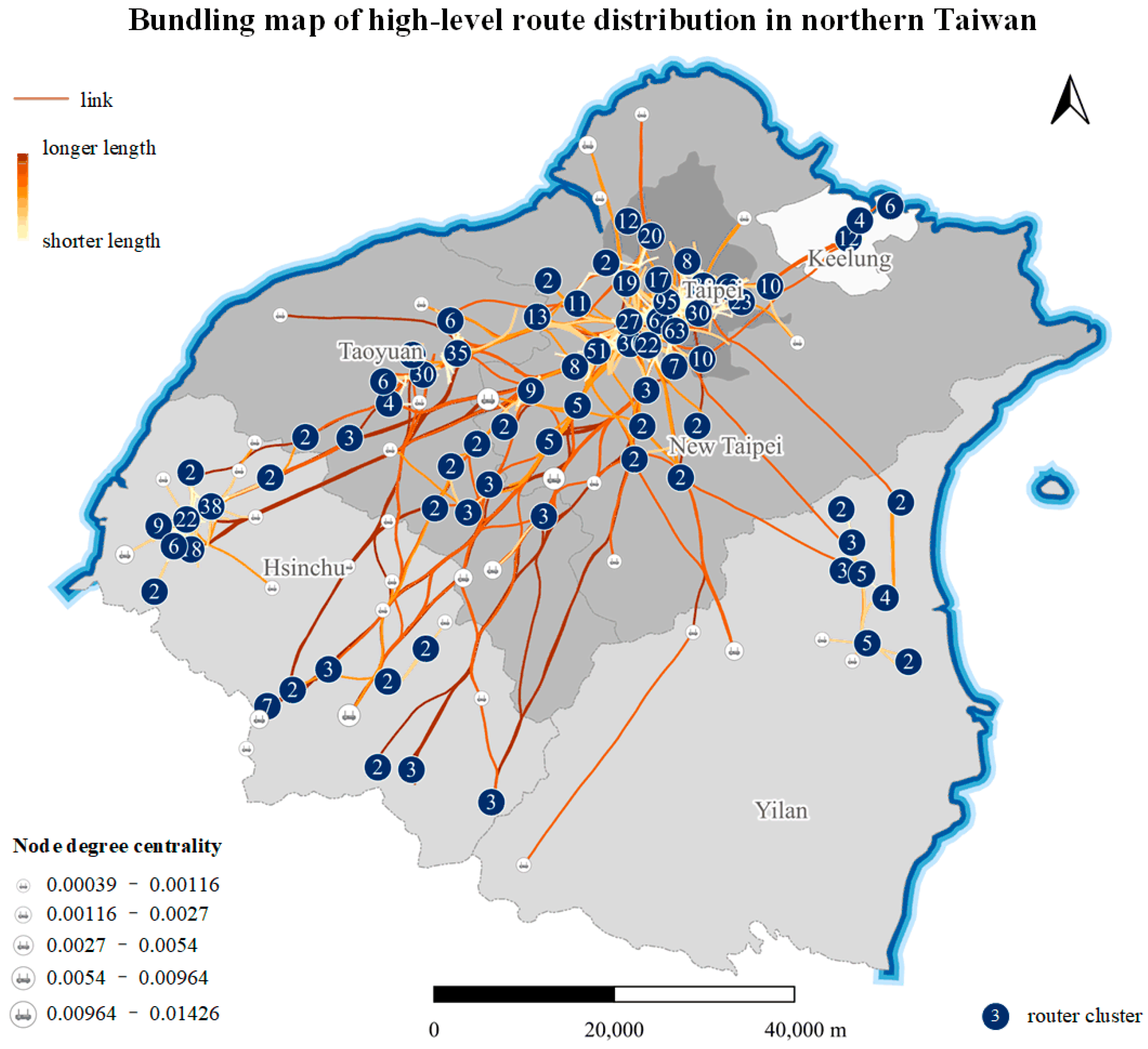
- Bundling map of high-level router distribution in northern Taiwan.
Due to the large number of edges in the router relationship data, the intertwined edges lead to the poor legibility and aesthetics of the map. For example, as shown in Figure 12 and Figure 13, the rigid, densely intertwined edges result in poor map visualization. We used the KDEEB algorithm to bundle the edges and symbolize and aggregate the nodes, with the final result shown in Figure 14. Compared with Figure 12, 14 is more concise and aesthetically pleasing, with improved legibility, effectively representing the distribution and relations in cyberspace.
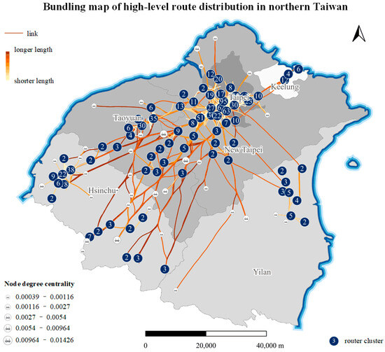
Figure 14.
Bundling map of high-level router distribution in northern Taiwan.
- 4.
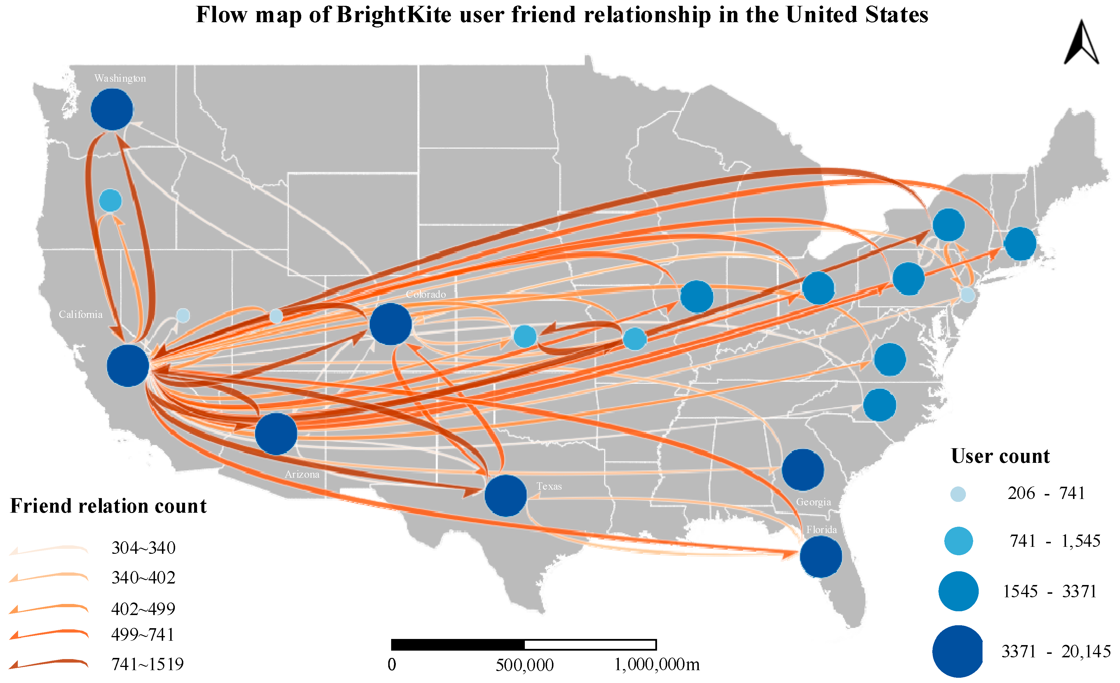
- Flow map of BrightKite user friend relationship in the United States.
By leveraging the aggregated BrightKite dataset, a flow map of the United States can be constructed [51], as illustrated in Figure 15.
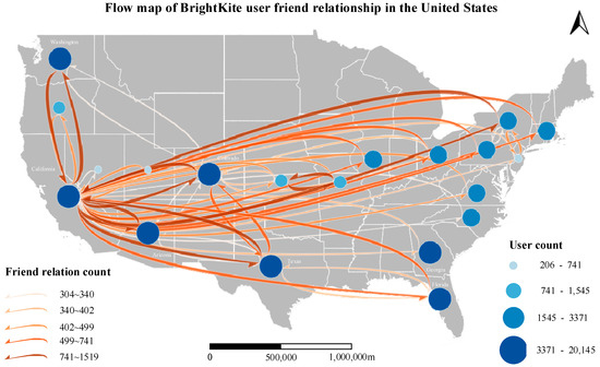
Figure 15.
Flow map of BrightKite user friend relationship in the United States.
The size and color of the nodes represent the number of BrightKite users in each state, while the color of the flows indicates the density of friendship connections between states. Through this flow map, the spatial distribution of BrightKite users and their interaction patterns can be visually illustrated. Specifically, Washington, California, Colorado, Arizona, Texas, Georgia, and Florida exhibit a higher concentration of BrightKite users. Notably, California has the highest frequency of friendship connections with other states, suggesting it is the most active hub for cross-state interactions.
- 5.
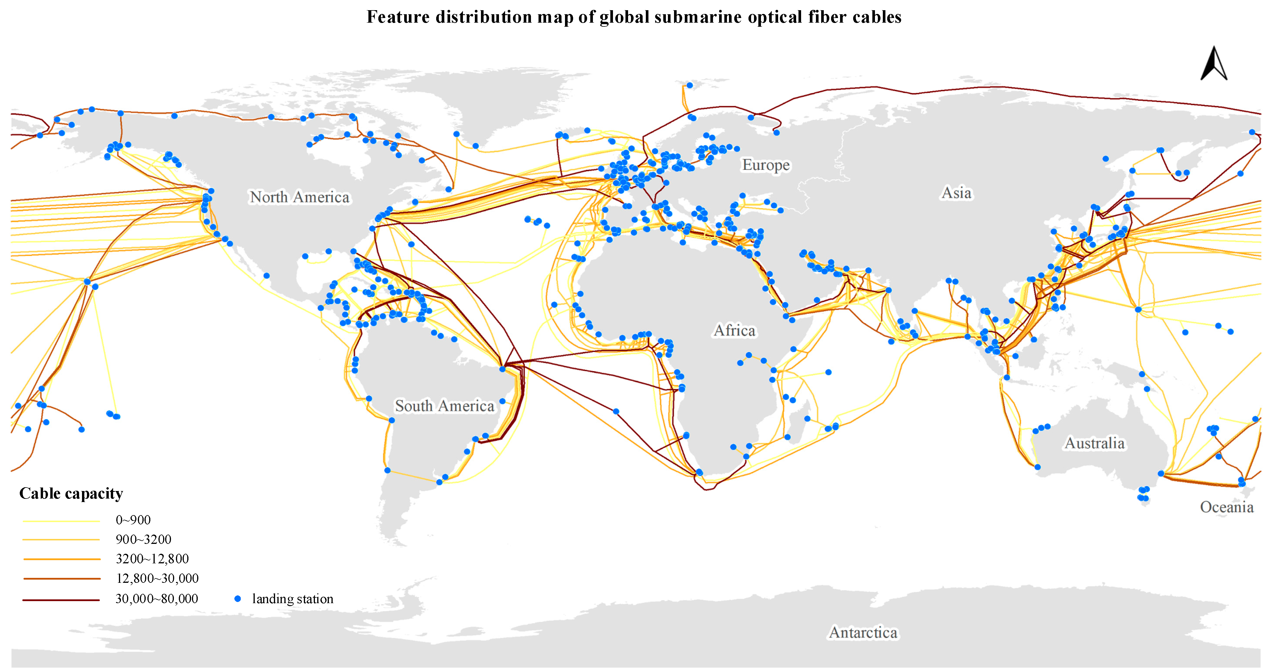
- Feature distribution map of global submarine fiber cables.
For the Cables dataset, to accurately depict the spatial locations of landing stations and submarine cables, this paper employs a feature distribution map to visualize the global spatial distribution of submarine cables. Specifically, the cable capacities are presented in a graded manner, as illustrated in Figure 16.
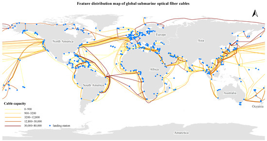
Figure 16.
Feature distribution map of global submarine fiber cables.
6. Conclusions
This paper introduces a data model and method framework for CMV. The integration of spatial and network data is realized through the “proxy mode”, enabling the visualization of cyberspace data through the steps of data processing, data rendering, and layout finalization. An experimental system was constructed on the basis of the symbol, model, and style libraries. Using the router relationship network data from northern Taiwan as an example, CMV experiments were conducted, including “zonal statistics”, “node-link” and “edge bundling”. The experimental results showed that the proposed data model can achieve a unified description and representation of cyber and space features, making it an innovative and effective cyberspace data model. In addition, the proposed method framework is well-suited for the map visualization of cyberspace data, effectively representing the distribution and relations of cyberspace features and also revealing the interaction patterns between cyberspace and geographic space.
As the integration of cyberspace and physical space deepens, gaining an intuitive understanding of cyberspace dynamics has become increasingly critical. This study aims to visualize the elements of cyberspace through mapping, thereby assisting relevant organizations and institutions in enhancing the targeted supervision and control of cyberspace while supporting the formulation and adjustment of related policies.
Nevertheless, this study has the following limitations:
- The paper does not evaluate the visualization effectiveness of the cyberspace map. Future research will study the evaluation from the perspectives of information density and visual load, among other aspects.
- The edge bundling method used in this study only aggregates edges based on spatial aesthetics standards and does not consider the semantic information of the edges. Therefore, the bundling results only improve the legibility and aesthetics of the cyberspace map but are less effective in revealing underlying patterns and knowledge.
- There are many types of cyberspace map visualizations, and only some of types were verified. Future efforts should be made to further implement additional visualization effects and explore more novel visualization methods.
Author Contributions
Conceptualization, Chenghu Zhou and Zheng Zhang; methodology, Zheng Zhang.; software, Zheng Zhang and Yibing Cao; validation, Minjie Chen, and Shaojing Fan.; formal analysis, Zheng Zhang; data curation, Shaojing Fan; writing—original draft preparation, Zheng Zhang; writing—review and editing, Minjie Chen; visualization, Zheng Zhang and Minjie Chen; supervision, Shaojing Fan; project administration, Zheng Zhang; funding acquisition, Chenghu Zhou and Zheng Zhang. All authors have read and agreed to the published version of the manuscript.
Funding
This research was funded by “the National Key Research and Development Program of China, grant number 2016YFB0502300”, “the National Key Research and Development Program of China, grant number 2021YFB3900900” and “the Natural Science Foundation of Henan Province, granted number 242300420624”.
Data Availability Statement
The data that support the findings of this study are available on request from the corresponding author [Z.Z.], but the data is only for personal research and cannot be publicly released. The experimental data was purchased through project funding and may involve copyright issues, so it cannot be made public temporarily.
Conflicts of Interest
The authors declare no conflict of interest.
Abbreviations
The following abbreviations are used in this manuscript:
| CMV | Cyberspace map visualization |
Appendix A
Table A1.
Classification system and examples of CMV.
Table A1.
Classification system and examples of CMV.
| Major Category | Description | Minor Category | Example | Map |
|---|---|---|---|---|
| Feature distribution map | Depict the spatial distribution of cyberspace features with precise geographic coordinates | Point distribution map | Distribution map of DNS in San Francisco | 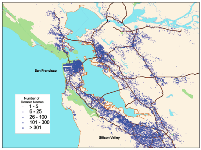 |
| Line distribution map | Global distribution map of submarine cables | 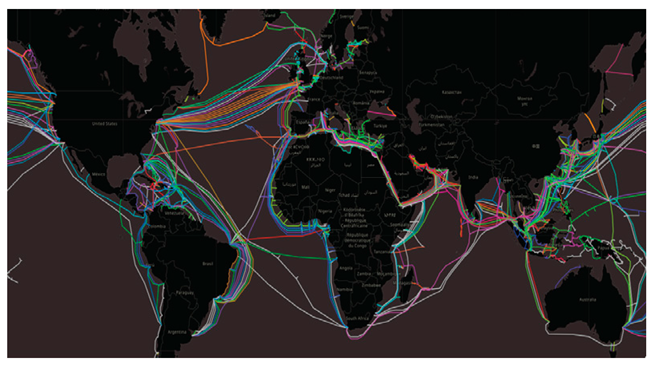 | ||
| Point and line distribution map | Distribution map of inland communication trunk lines and base stations | 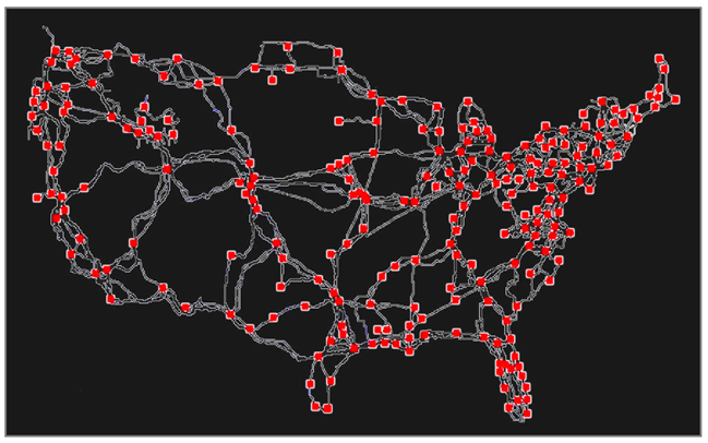 | ||
| Node-link map | Depict the flow, direction, trend, association or other information of cyberspace elements via the node-link method | Flow map | Telecom flow map of TeleGeography | 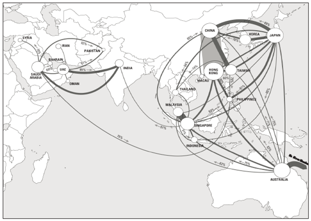 |
| Network map | Network map of UUNet backbone | 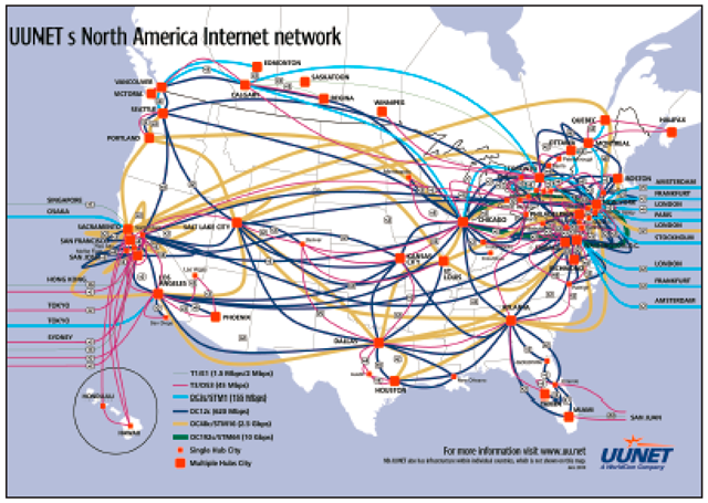 | ||
| Bundling map | Bundling map of US airlines | 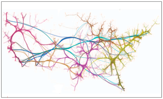 | ||
| Direction map | Attack and defense map of DDoS | 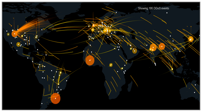 | ||
| Statistical thematic map | Depict the statistical information of cyberspace elements by charts or symbols | Statistical thematic map by point | Cluster map of global POP | 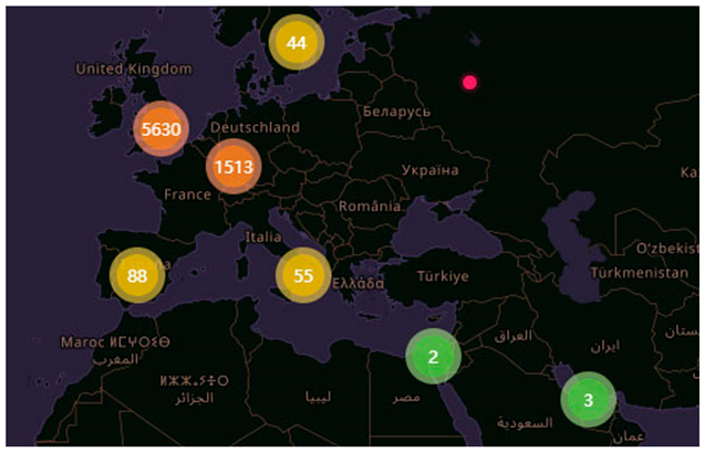 |
| Statistical thematic map by area | Map of internet regional connectivity | 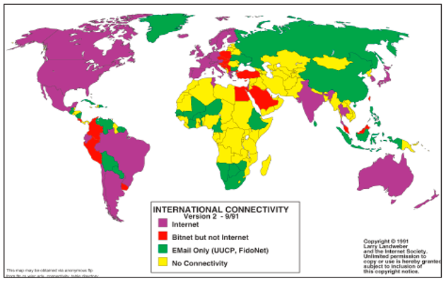 | ||
| Heatmap | Heatmap of IP distribution | 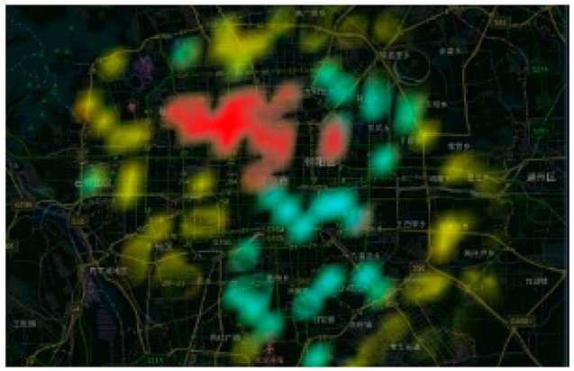 | ||
| Cartogram map | Depict the information of cyberspace elements by distorting the geographic space | Distance cartogram | Map of provincial trunk network | 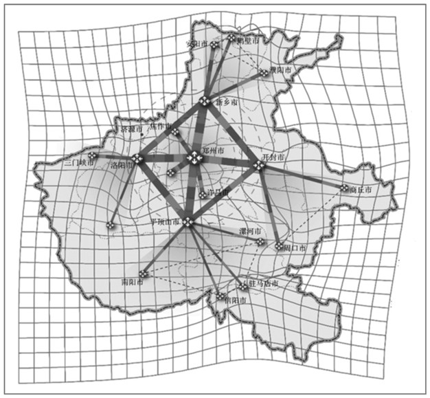 |
| Area cartogram | Distribution map of global internet user | 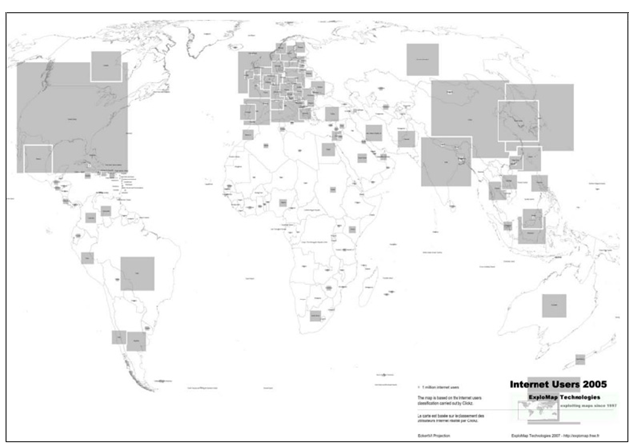 |
References
- Guo, H.S. Cyberspace Security Strategy, 1st ed.; Aviation Industry Press: Beijing, China, 2016; pp. 1–2. [Google Scholar]
- Sun, Z.; Lu, Z.; Wang, Y. The geography of cyberspace: Review and prospect. Adv. Earth Sci. 2007, 22, 1005–1011. [Google Scholar]
- Zhou, Y.; Xu, Q.; Luo, X.Y.; Liu, F.L.; Zhang, L.; Hu, X.F. Research on definition and technological system of cyberspace surveying and mapping. Comput. Sci. 2018, 45, 1–7. [Google Scholar]
- Bakis, H. Understanding the geocyberspace: A major task for geographers and planners in the next decade. NETCOM Réseaux Commun. Territ./Net. Commun. Stud. 2001, 15, 9–16. [Google Scholar] [CrossRef]
- Gao, C.; Guo, Q.; Jiang, D.; Wang, Z.; Fang, C.; Hao, M. Theoretical basis and technical methods of cyberspace geography. J. Geogr. Sci. 2019, 29, 1949–1964. [Google Scholar] [CrossRef]
- Fraser Taylor, D.R.; Caquard, S. Cybercartography: Maps and mapping in the information era. Int. J. Geogr. Inf. Geovis. 2006, 41, 1. [Google Scholar] [CrossRef]
- Li, X.; Yang, F.; Wang, L.N.; Yu, X.K.; Fei, T.; Jiang, N. A survey of mapping methods for cyberspace. J. Geomat. Sci. Technol. 2019, 36, 620–626+631. [Google Scholar]
- Zhang, L.; Wang, G.X.; Jiang, B.C.; Zhang, L.T.; Ma, L. A review of visualization methods for cyberspace maps. Geomat. Inf. Sci. Wuhan Univ. 2022, 47, 2113–2122. [Google Scholar]
- Dodge, M.; Kitchin, R. Geographies of cyberspace. In Atlas of Cyberspace, 1st ed.; Routledge: London, UK, 2003; pp. 52–64. [Google Scholar]
- December, J. A Cybermap Gazetteer: Maps of the On-Line World for Browsing and Business. Global Telecommunications Traffic Statistics & Commentary; TeleGeography, Inc.: Washington, DC, USA, 1995; p. 210. [Google Scholar]
- Tsou, M.H.; Kim, I.H.; Wandersee, S.; Lusher, D.; Li, A.; Spitzberg, B.; Gupta, D.; Gawron, J.M.; Mason, J.S.; Yang, J.-A.; et al. Mapping ideas from cyberspace to realspace: Visualizing the spatial context of keywords from web page search results. Int. J. Digit. Earth 2014, 7, 316–335. [Google Scholar] [CrossRef]
- Wang, Y.; Li, X.; Ren, G.M.; Tian, Z.K. Overview of Global Network Space Mapping and Mapping Research. Inf. Technol. Netw. Secur. 2019, 38, 1–6. [Google Scholar]
- Chen, Y.H.; Jiang, N.; Cao, Y.B.; Zi, L. Application of cartography theory in cartography of cyberspace map. J. Geomat. Sci. Technol. 2020, 37, 301–306. [Google Scholar]
- He, J.; Zheng, Z.; Lei, S. Research on cyberspace map technology in the electric power industry. In Proceedings of the 2023 4th International Conference on Big Data Economy and Information Management, Zhengzhou, China, 8 December 2023. [Google Scholar]
- Zhu, X.Q.; Zhu, C.; Ding, Z.Y.; Liu, B.; Liu, Y. Map Modeling and Intelligence Terrain Analysis Method for Cyberspace. J. Command Control 2022, 8, 294–302. [Google Scholar]
- Zhang, L.; Wang, G.X.; You, X.; Liu, Z.; Ma, L.; Tian, J.; Su, M. Research on the Cyberspace Map and Its Conceptual Model. ISPRS Int. J. Geo-Inf. 2023, 12, 353. [Google Scholar] [CrossRef]
- Jiang, B.C.; Si, D.Y.; Liu, J.X.; Ren, Y.; You, X.; Cao, Z.; Li, J.W. Cyberspace surveying and mapping. J. Geo-Inf. Sci. 2024, 26, 848–865. [Google Scholar]
- Zhang, Z.; Zhou, C.; Chen, M.; Fan, S. A skeleton extraction method for large-scale spatial interaction networks considering spatial distribution characteristics. Int. J. Geogr. Inf. Sci. 2025, 39, 1–27. [Google Scholar] [CrossRef]
- Guo, D.; Zhu, X. Origin-destination flow data smoothing and mapping. IEEE T. Vis. Comput. Gr. 2014, 20, 2043–2052. [Google Scholar] [CrossRef]
- Zhu, X.; Guo, D. Mapping large spatial flow data with hierarchical clustering. Tran. GIS 2014, 18, 421–435. [Google Scholar] [CrossRef]
- Jenny, B.; Stephen, D.M.; Muehlenhaus, I.; Marston, B.E.; Sharma, R.; Zhang, E.; Jenny, H. Force-directed layout of origin–destination flow maps. Int. J. Geogr. Inf. Sci. 2017, 31, 1521–1540. [Google Scholar] [CrossRef]
- Jenny, B.; Stephen, D.M.; Muehlenhaus, I.; Marston, B.E.; Sharma, R.; Zhang, E.; Jenny, H. Design principles for origin–destination flow maps. Cartogr. Geogr. Inf. Sci. 2018, 45, 62–75. [Google Scholar] [CrossRef]
- Zhu, X.; Guo, D.; Koylu, C.; Chen, C. Density-based multiscale flow mapping and generalization. Comput. Environ. Urban 2019, 77, 101359. [Google Scholar] [CrossRef]
- Wang, Y.X.; Li, S.M.; Zhang, X.L.; Zhang, C.T.; Wang, R.H. Visualization of cyberspace information based on composite distance cartogram. J. Inf. Eng. Univ. 2020, 21, 334–339+360. [Google Scholar]
- Liu, L.H.; Shi, Q.S.; Zhou, Y.; Hu, X.F.; Xu, Q. Visualization and analysis of Cyberspace Metaphor Gosper Map. J. Geo-Inf. Sci. 2024, 26, 144–157. [Google Scholar]
- Holten, D.; Van Wijk, J.J. Force-directed edge bundling for graph visualization. In Computer Graphics Forum; Blackwell Publishing Ltd.: UK, Oxford, 2009. [Google Scholar]
- Ersoy, O.; Hurter, C.; Paulovich, F.; Cantareiro, G.; Telea, A. Skeleton-based edge bundling for graph visualization. IEEE Trans. Vis. Comput. Gr. 2011, 17, 2364–2373. [Google Scholar] [CrossRef] [PubMed]
- Hurter, C.; Ersoy, O.; Telea, A. Graph bundling by kernel density estimation. In Computer Graphics Forum; Blackwell Publishing Ltd.: Oxford, UK, 2012. [Google Scholar]
- Zou, L.; Brooks, S. A dynamic approach for presenting local and global information in geospatial network visualizations. Geoinformatica 2019, 23, 733–757. [Google Scholar] [CrossRef]
- Jiang, B.; You, X.; Li, K.; Li, T.; Wang, X.; Si, D. Virtual geo-cyber environments: Metaphorical visualization of virtual cyberspace with geographic knowledge. Int. J. Digit. Earth 2024, 17, 2324959. [Google Scholar] [CrossRef]
- Si, D.; Jiang, B.; Xia, Q.; Li, T.; Wang, X.; Liu, J. Cyber Potential Metaphorical Map Method Based on GMap. ISPRS Int. J. Geo-Inf. 2025, 14, 46. [Google Scholar] [CrossRef]
- Ai, T.H. Maps adaptable to represent spatial cognition. J. Remote Sens-Prc. 2008, 12, 347–354. [Google Scholar]
- Dodge, M. Understanding Cyberspace Cartographies: A Critical Analysis of Internet Infrastructure Mapping. Ph.D. Thesis, University of London, London, UK, 2008. [Google Scholar]
- Jiang, B.; Ormeling, F.J. Cybermap: Map for cyberspace. Cartogr. J. 1997, 34, 111–116. [Google Scholar] [CrossRef]
- Ai, T.H. Development of cartography driven by big data. J. Geomat. 2016, 41, 1–7. [Google Scholar]
- Jiang, B.; Ormeling, F. Mapping cyberspace: Visualizing, analyzing and exploring virtual worlds. Cartogr. J. 2000, 37, 117–122. [Google Scholar] [CrossRef]
- Zhang, L.; Zhou, Y.; Shi, Q.S. Cyberspace map tightly coupled with geographic space. J. Cyber Secur. 2018, 3, 63–72. [Google Scholar]
- Fang, Z.; Li, Q.; Zhang, X.; Shaw, S.L. A GIS data model for landmark-based pedestrian navigation. Int. J. Geogr. Inf. Sci. 2012, 26, 817–838. [Google Scholar] [CrossRef]
- Mayr, H.C.; Thalheim, B. The triptych of conceptual modeling: A framework for a better understanding of conceptual modeling. Softw. Syst. Model. 2021, 20, 7–24. [Google Scholar] [CrossRef]
- Van, L.D.; Wijshoff, V.; Joosen, W. A study of NoSQL query injection in Neo4j. Comput. Secur. 2024, 137, 103590. [Google Scholar]
- Chaves-Fraga, D.; Priytna, F.; Santana-Perez, I.; Corcho, O. Virtual Statistics Knowledge Graph Generation from CSV Files; IOS Press: Amsterdam, The Netherlands, 2018. [Google Scholar]
- Bruns, A. How long is a tweet? Mapping dynamic conversation networks on Twitter using Gawk and Gephi. Inform. Commun. Soc. 2012, 15, 1323–1351. [Google Scholar] [CrossRef]
- Olfat, H.; Kalantari, M.; Rajabifard, A.; Senot, H.; Williamson, I.P. A GML-based approach to automate spatial metadata updating. Int. J. Geogr. Inf. Sci. 2013, 27, 231–250. [Google Scholar] [CrossRef]
- Boeing, G. Street network shapefiles, node/edge lists, and graph files. Comput. Comput. Environ. Urban 2017, 65, 126–139. [Google Scholar] [CrossRef]
- Krnc, M.; Škrekovski, R. Group degree centrality and centralization in networks. Mathematics 2020, 8, 1810. [Google Scholar] [CrossRef]
- Newman, M.E.J. A measure of betweenness centrality based on random walks. Soc. Netw. 2005, 27, 39–54. [Google Scholar] [CrossRef]
- Du, Y.; Gao, C.; Chen, X.; Hu, Y.; Sadiq, R.; Deng, Y. A new closeness centrality measure via effective distance in complex networks. Chaos Interdiscip. J. Nonlinear Sci. 2015, 25, 033112. [Google Scholar] [CrossRef]
- Bonacich, P. Some unique properties of eigenvector centrality. Soc. Netw. 2007, 29, 555–564. [Google Scholar] [CrossRef]
- Mark, B.; Otfried, C.; Marc, K.; Mark, O. Computational Geometry Algorithms and Applications; Springer: Berlin/Heidelberg, Germany, 2008. [Google Scholar]
- Cho, E.; Myers, S.A.; Leskovec, J. Friendship and Mobility: User Movement in Location-Based Social Networks. In Proceedings of the 17th ACM SIGKDD International Conference on Knowledge Discovery and Data Mining, San Diego, CA, USA, 21–24 August 2011. [Google Scholar]
- Koylu, C.; Tian, G.; Windsor, M. Flowmapper. org: A web-based framework for designing origin–destination flow maps. J. Maps. 2023, 19, 1996479. [Google Scholar] [CrossRef]

Disclaimer/Publisher’s Note: The statements, opinions and data contained in all publications are solely those of the individual author(s) and contributor(s) and not of MDPI and/or the editor(s). MDPI and/or the editor(s) disclaim responsibility for any injury to people or property resulting from any ideas, methods, instructions or products referred to in the content. |
© 2025 by the authors. Published by MDPI on behalf of the International Society for Photogrammetry and Remote Sensing. Licensee MDPI, Basel, Switzerland. This article is an open access article distributed under the terms and conditions of the Creative Commons Attribution (CC BY) license (https://creativecommons.org/licenses/by/4.0/).