Abstract
In the last two decades, South Korea has seen an increase in extreme rainfall coinciding with the proliferation of impermeable surfaces due to urban development. When underground drainage systems are overwhelmed, pluvial flooding can occur. Therefore, recognizing drainage systems as key flood-conditioning factors is vital for identifying flood-prone areas and developing predictive models in highly urbanized regions. This study evaluates and maps urban pluvial flood susceptibility in Seoul, South Korea using the machine learning techniques such as logistic regression (LR), random forest (RF), and support vector machines (SVM), and integrating traditional flood conditioning factors and drainage-related data. Together with known flooding points from 2010 to 2022, sixteen flood conditioning factors were selected, including the drainage-related parameters sewer pipe density (SPD) and distance to a storm drain (DSD). The RF model performed best (accuracy: 0.837, an area under the receiver operating characteristic curve (AUC): 0.902), and indicated that 32.65% of the study area has a high susceptibility to flooding. The accuracy and AUC were improved by 7.58% and 3.80%, respectively, after including the two drainage-related variables in the model. This research provides valuable insights for urban flood management, highlighting the primary causes of flooding in Seoul and identifying areas with heightened flood susceptibility, particularly relating to drainage infrastructure.
1. Introduction
Floods are typically triggered by heavy rainfall, which either runs off on the ground surface, overflows from drainage systems, or infiltrates into the soil. In natural landscapes such as mountains or farmland, runoff flows towards river systems, during which some of the water infiltrates into the soil or is retained by vegetation, reducing the volume reaching rivers. Meanwhile, in urban areas with drainage systems connected to river systems, runoff is directed into these waterways unless special facilities are in place to store and manage it [1]. However, due to the increase in urban impermeable surfaces caused by population growth, the capacity of natural and urban drainage systems to manage stormwater runoff during intense rainfall events has decreased, leading to widespread inundation and flooding [2]. Such events significantly impact buildings, infrastructure, and other aspects of urban settlements, both directly and indirectly. Thus, it is crucial to understand the spatial distribution of urban flood susceptibility to make appropriate decisions regarding land use, infrastructure development, emergency response planning, and insurance pricing.
Over the last two decades, Seoul, South Korea, has witnessed a consistent increase in average annual precipitation and the frequency of days with rainfall exceeding 80 mm/day, resulting in an increased frequency and severity of urban flooding. The city has experienced several significant floods in the 21st century, with two of the most severe events occurring in 2010 and 2011. The 2010 event was characterized by a rainfall of 260 mm/day and caused the overflow of Cheonggye Stream, leading to extensive damage to buildings and other infrastructure. In the 2011 event, more than 156.1 mm of rainfall occurred in two hours, surpassing the anticipated 100-year rainfall projection. These events revealed the inadequacy of existing flood prevention measures in Seoul.
On 9 August 2022, Seoul experienced its most damaging flood on record (overtaking the 2010 and 2011 events). This extreme event was caused by the heaviest rainfall in over a century, with an hourly precipitation rate of 141.5 mm/h (surpassing the previous record of 118.6 mm/h set in 1942), which overwhelmed the city’s sewer system. The flooding affected thousands of buildings and caused several billion dollars of property damage [3]. The Gangnam area of Seoul was among the most affected areas. Although this area is naturally predisposed to flooding due to its relatively low elevation, another significant factor contributing to the extensive inundation was drainage problems due to the backflow of stormwater caused by elevated water levels in the Banpo Stream and overwhelmed sewer pipes in the Gangnam region [4]. Furthermore, rainwater catchment facilities were widely compromised by debris accumulation, hindering the drainage of stormwater and thus exacerbating flooding incidents.
The Gangnam flood resulted in the loss of eight lives, again underscoring the deficiency of flood mitigation measures in Seoul. A notable concern that has been raised is the absence of a comprehensive flood risk map for the city, which hampers the assessment of potential flood risks. In 2021, South Korea’s Ministry of Environment made fluvial flood risk maps publicly available to inform communities about areas prone to flooding in the event of an overflow from nearby streams or rivers due to extreme precipitation. However, of the 25 districts of Seoul, only nine have complete and accessible pluvial flood risk maps, while others have incomplete or nonexistent maps. Also, the government-provided flood risk maps are not regularly updated and do not incorporate changes in urban development and the built environment [5].
Researchers have modeled the urban flood susceptibility of Seoul using various flood conditioning factors and research methodologies [6,7,8,9,10]. While studies conducted by Lee et al. in 2017 [6] and in 2018 [7] used similar geospatial variables such as geomorphology, lithology, land use, and soil type, they employed distinct methodologies. The former [6] used random forest (RF) and boosted-tree models to construct classification and regression algorithms to map the urban flood susceptibility of Seoul, while the latter [7] applied basic statistical data-based models such as frequency ratio and logistic regression (LR). Similarly, Lee and Kim [8] identified flood-prone areas in Seoul by integrating topographic and hydrological factors using LR. In another approach, Narimani et al. [9] created a flood susceptibility model for Seoul by incorporating rainfall and satellite-based land use data with the analytic hierarchy process (AHP). Meanwhile, Lei et al. [10] expanded on the modeling approach of [9] by using deep-learning approaches such as convolutional neural networks (CNN) and recurrent neural networks (RNN). The application of machine-learning algorithms has significantly enhanced the accuracy and efficiency of flood susceptibility mapping compared to traditional methods, contributing to more effective disaster management and mitigation strategies. Therefore, these studies demonstrate the importance of integrating ML methodologies with diverse datasets to enhance flood susceptibility mapping and risk assessment.
However, previous flood susceptibility maps of Seoul often neglected the impact of the city’s drainage system on flooding, mainly due to the confidential nature of data on this system. In urban environments, the presence of impermeable in road networks (e.g., concrete and asphalt) prevents stormwater from infiltrating into the ground, resulting in increased surface runoff. Ideally, this runoff should be efficiently directed into underground drainage systems through stormwater inlets and manholes before ultimately draining into nearby rivers or streams. However, during extreme precipitation, the volume of surface runoff can surpass the capacity of drainage systems, leading to sewer backflow [11]. This backflow redirects the runoff onto streets and roads, which can cause inundation and flooding.
It is critical to acknowledge the significant role of urban stormwater drainage systems in flooding and integrate them into flood susceptibility models to accurately identify flood-prone areas. Therefore, this study aims to evaluate and map urban pluvial flood susceptibility in Seoul using three machine learning (ML) techniques—LR, RF, and support vector machines (SVM)—together with commonly used flood conditioning factors, and information on the city’s drainage system. By integrating traditional flood conditioning factors with drainage-related data, this study addresses a critical research gap in previous flood susceptibility research in Seoul, which largely overlooked the role of drainage infrastructure. Specifically, it investigates the extent to which drainage-related variables affect the occurrence and spatial distribution of flooding events in Seoul. The findings offer novel insights into how drainage systems affect urban flood risk. The following section presents a literature review. Section 3 describes the data and methods. Section 4 and Section 5 present the results and discussion, respectively. Finally, concluding remarks are provided.
2. Literature Review
2.1. Urban Flooding
Urban flooding has become a global concern. Urbanization replaces permeable soil and vegetation with impermeable structures, which increases the flood risk. Moreover, intense rainfall linked to climate change further elevates this risk [12,13]. Urban flooding can be categorized into two types: fluvial flooding, caused by the overflow of urban streams and rivers, and pluvial flooding, caused by the excessive runoff of surface rainwater due to poor stormwater drainage and sewer systems [14].
The proliferation of impervious surfaces has increased the susceptibility of urban drainage and sewer systems to becoming overwhelmed during intense rainfall events, leading to widespread flooding [15]. Engineering structures such as embankments and levees mitigate river overflow but increase the impermeable surface, which can cause inundation in low-lying areas. Poorly managed urban drainage systems exacerbate these effects by reducing the drainage capacity and thus increasing localized flooding risks.
In rapidly urbanizing small and medium-sized towns, the neglect of natural drainage systems and cross-drainage structures worsens flooding. Small urban streams are particularly vulnerable to overflowing, experiencing rapid surges during heavy rainfall due to the accelerated runoff and shorter concentration times. Inadequate maintenance and improper waste disposal can further exacerbate flood risks by obstructing drainage channels [16].
Urban areas are increasingly vulnerable to extreme weather events, particularly localized torrential downpours and floods, due to high population density and insufficient infrastructure [17]. Flooding directly and indirectly impacts urban infrastructure, including underground spaces such as subways and basements. Adapting existing structures in flood-prone areas is challenging, especially in developing nations grappling with climate change. While new constructions can integrate flood-resilient designs, stricter regulations are needed to limit development in high-risk areas. Flood risk varies with the urbanization level, thus necessitating dynamic flood risk assessments. Flood risk maps are crucial for identifying vulnerable areas, guiding mitigation efforts, and informing resource allocation, while regular updates and monitoring are required to ensure effective policymaking and resource management.
2.2. Modeling Flood Susceptibility
Various models are commonly employed to assess the flood risk and susceptibility, including hydrological-based, knowledge-based, and machine-learning (ML)-based models [18,19]. These models have traditionally treated river basins as single, linear, and predictable systems. However, GIS-based hydrological models have recently been developed—such as the River Basin Simulation Model (RIBASIM), the Hydrologic Engineering System’s Hydrologic Modeling System (HEC-HMS) and the River Analysis System (HEC-RAS), and the Storm Water Management Model (SWMM)—which incorporate spatial representations of hydrological features into forecasting algorithms [20].
Some studies have explored the use of knowledge-based models for evaluating flood susceptibility, such as multicriteria decision analysis (MCDA) [21,22,23] and the analytic hierarchy process (AHP) [9,24,25]. However, these models are limited by their inherent subjectivity as they require input from experts who interpret and make assumptions about model inputs.
However, ML-based models have recently emerged as a promising approach for examining the relationships between flood conditioning factors and environmental variables. These models effectively recognize complex patterns and correlations that conventional methods may overlook [26]. For instance, the LR model predicts flood susceptibility by establishing a connection between floods and independent variables using a formula derived from a set of independent variables. LR is valued for its consistency in identifying key factors contributing to flood occurrence, and has been used to predict flood susceptibility in previous studies [7,27,28,29]. Additionally, the RF model, has been employed for flood susceptibility mapping in various studies [6,15,30,31,32,33]. It is known for its high accuracy, and its ability to recognize outliers and anomalies, which reduces data overfitting. The SVM model has also been used in flood susceptibility mapping due to its ability to handle complex functions and structured and semi-structured datasets [32,34,35,36]. The LR, RF, and SVM techniques have been successfully used in flood susceptibility modeling and mapping, both in Seoul [6,7,10,28,29] and other regions worldwide [15,27,30,32,33,34,35,36,37,38]. These methods are simple to execute, require minimal programming knowledge, and can effectively handle large, complex datasets, making them practical tools for investigating the factors contributing to flood risk and susceptibility.
However, the effectiveness of ML models depends on factors such as data quality, feature and parameter selection, and validation. Therefore, careful implementation, continuous updates, and regular validation are essential to ensure the reliability and effectiveness of ML algorithms for flood susceptibility analysis.
3. Materials and Methods
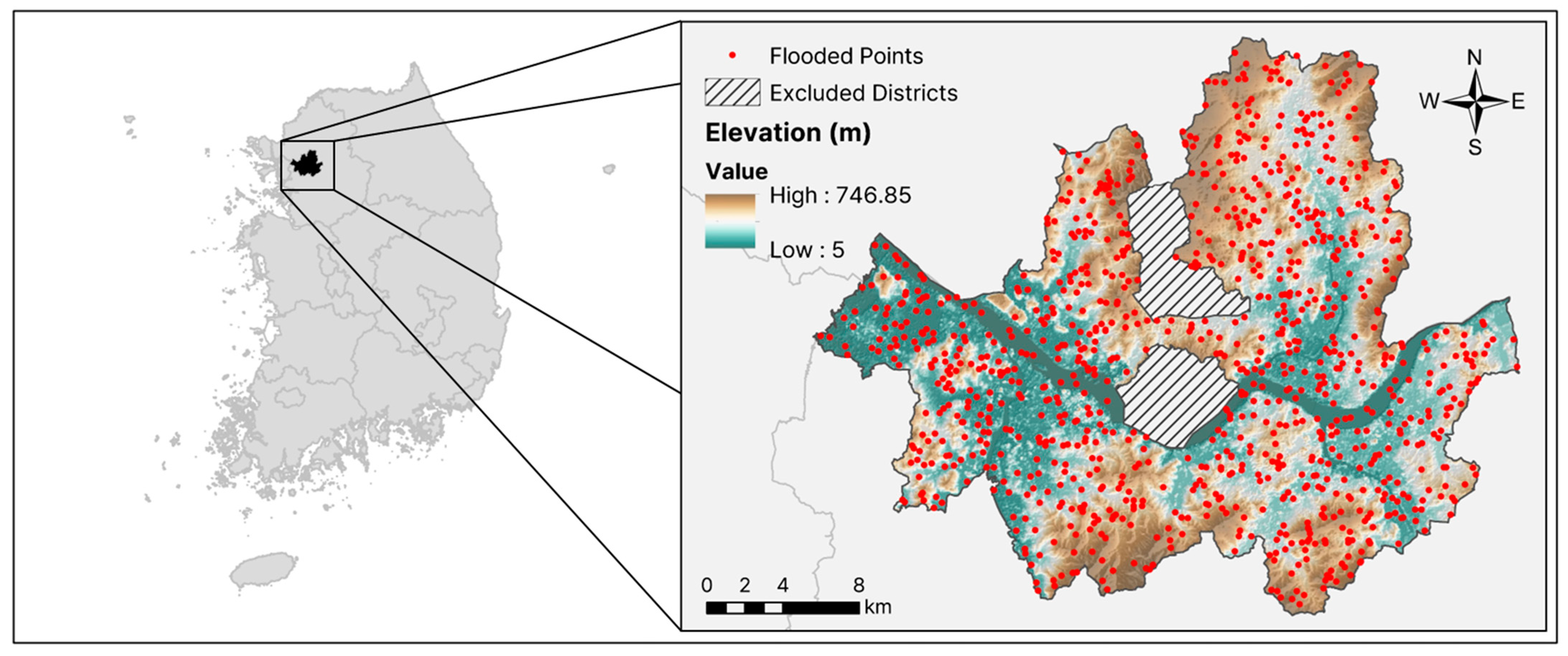
The study area is Seoul, the capital city of South Korea, which is situated between 37.41° and 37.72° N latitude and between 126.73° and 127.27° E longitude. Seoul has a monsoon climate, with an annual rainfall of 1300 to 1500 mm [39]. Approximately 65% of this precipitation occurs during summer, leading to a greater potential for flooding in this season [10].
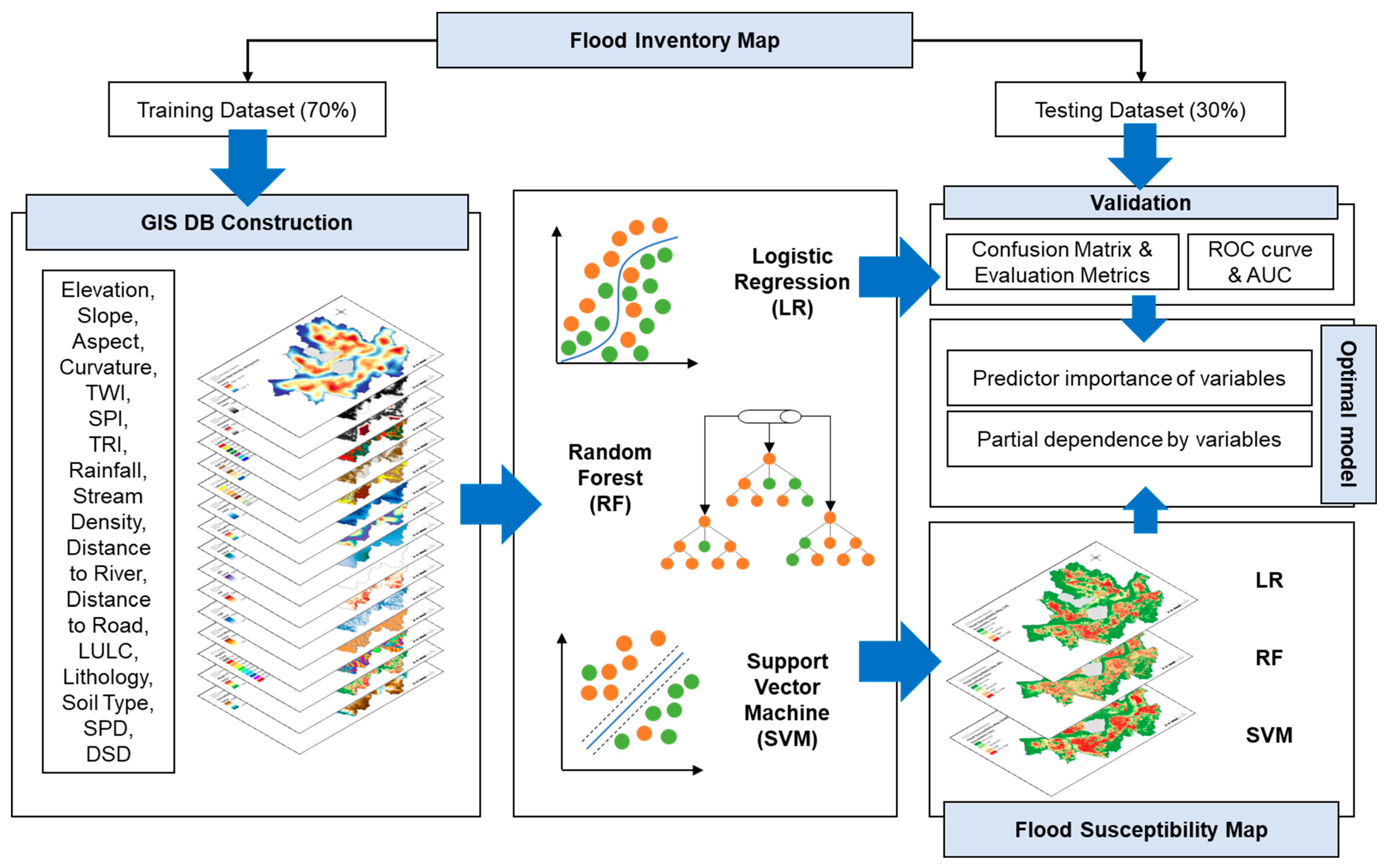
Figure 1 presents a flowchart of the research process, outlining the sequential steps involved in model training, validating, and evaluation, and selecting the optimal model for generating flood susceptibility maps.
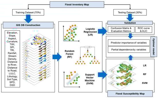
Figure 1.
A flowchart outlining the research performed in this study.
3.1. Spatial Datasets
The fundamental assumption underlying flood susceptibility modeling is that future floods are likely to occur in similar locations to past floods [32]. In this study, a flood inventory map was developed using flooding data between 2010 and 2022 provided by the Seoul Metropolitan Government. To increase accuracy and minimize algorithmic errors, this map was transformed into point data through centroid calculations.
Of the 15,956 identified flooded points, 1000 were randomly selected, and assigned a code number of “1” to indicate the presence of a flood. Similarly, 1000 non-flooded points were randomly chosen and were given a code number of “0”. Figure 2 provides an overview of the study area along with the locations of the flooded points.
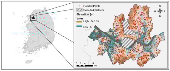
Figure 2.
An overview of the study area showing the selected flooded points recorded between 2010 and 2022, derived from the Seoul Metropolitan Government database.
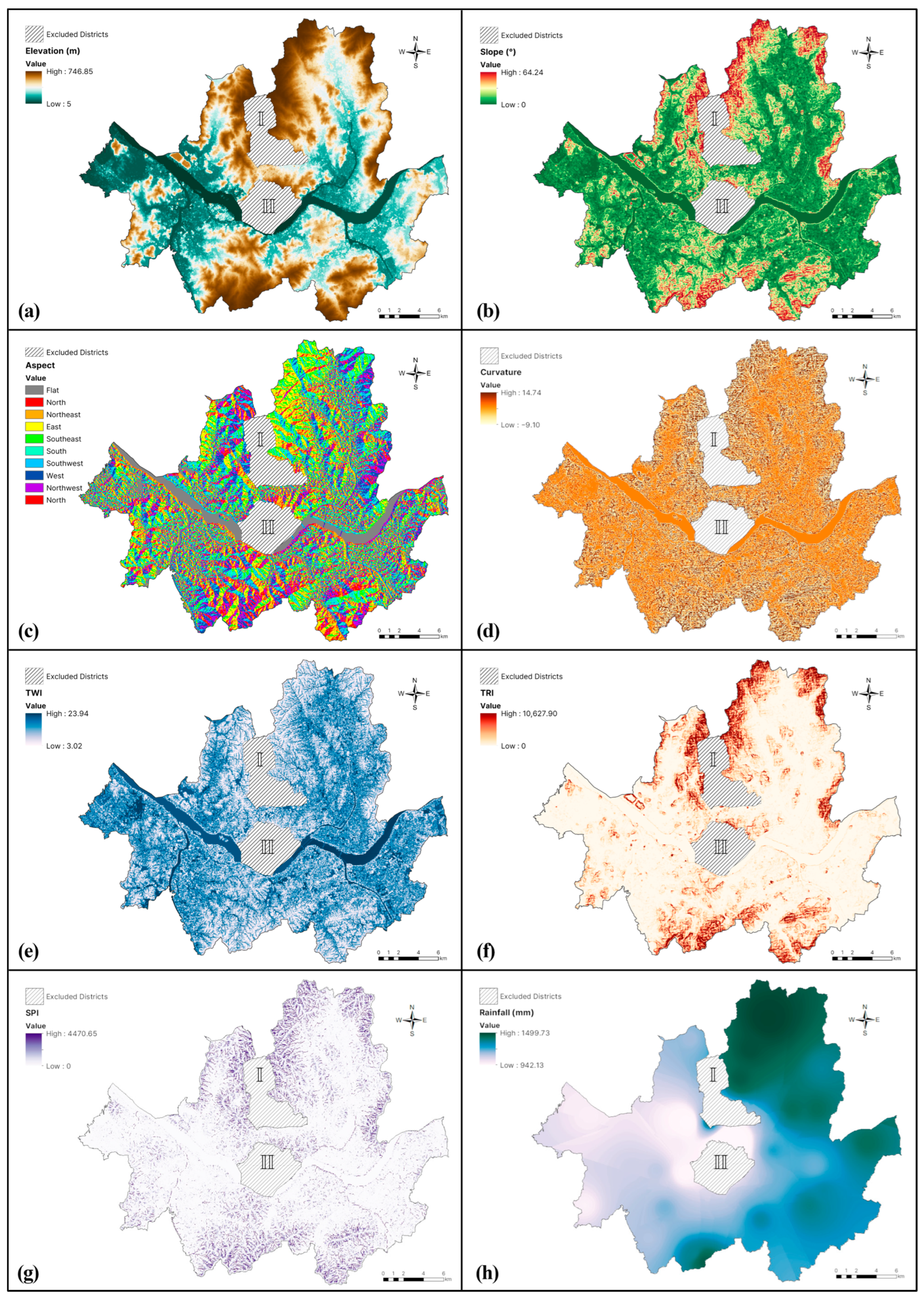
The following 16 variables were selected as flood conditioning factors based on the previous literature sources, data availability, and field observations (see Table 1 and Figure 3): elevation, slope, aspect, curvature, the topographic wetness index (TWI), the terrain roughness index (TRI), the stream power index (SPI), rainfall, stream density, sewer pipe density (SPD), distance to a river, distance to a road, distance to a storm drain (DSD), lithology, land use and land cover (LULC), and soil type. These variables were subsequently applied to three ML models and, in combination with the extracted flooded points, were used to generate flood susceptibility maps. Table 1 shows the data sources for each flood conditioning factor and Figure 3 shows thematic maps for each explanatory variable.

Table 1.
The data sources for each flood conditioning factor employed in this research.

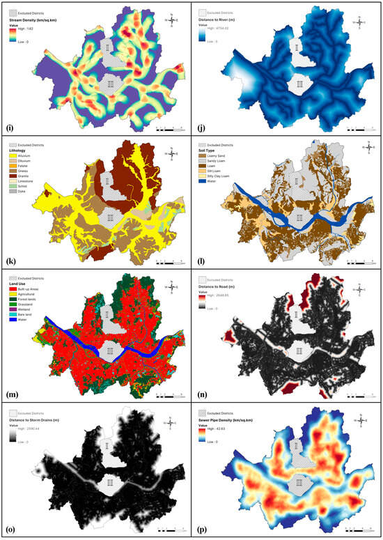
Figure 3.
Thematic maps illustrating the flood conditioning factors in the Seoul Metropolitan Area considered in this research: (a) elevation, (b) slope (in degrees), (c) aspect, (d) curvature, (e) the topographic wetness index (TWI), (f) the terrain roughness index (TRI), (g) the stream power index (SPI), (h) rainfall, (i) stream density, (j) distance to river, (k) lithology, (l) soil type, (m) land use and land cover, (n) distance to a road, (o) distance to a storm drain (DSD), and (p) sewer pipe density (SPD). (I) and (II) show the districts of Jongro-gu and Yongsan-gu, which were excluded from the analysis due to lack of data availability.
Topographic factors were extracted from a 30 m resolution DEM constructed using Shuttle Radar Topography Mission (SRTM) data provided by the National Aeronautics and Space Administration (NASA) Jet Propulsion Laboratory (JPL). This spatial resolution was chosen based on studies showing that DEMs with a 30 m resolution demonstrated a comparable accuracy for flood susceptibility mapping compared to higher-resolution DEMs [40,41].
The elevation can be directly related to flooding as areas located at lower elevations tend to be more susceptible to runoff [35,42]. The slope angle can also affect flood occurrence as it impacts the speed and velocity of runoff, with gentle slopes resulting in slower runoff and thus being more prone to significant flooding than steep slopes. Meanwhile, the aspect (slope direction) influences the direction of runoff [43], which can also influence flood occurrence. Moreover, areas with concave or negative curvatures (change of slope inclination) have a greater flood risk as they retain more water [10].
The TWI is commonly used to quantify the topographic control on hydrological processes [44] and is defined as follows:
where is the drained area per unit contour length at a certain point and is the surface slope in degrees. As the TWI is indirectly related to the slope, it is directly related to the flood risk as gentler slopes (which are more likely to accumulate water and thus experience flooding) have higher TWIs [45].
The TRI is the mean elevation change between a grid cell and the eight surrounding grid cells. It is calculated as follows:
where is the elevation of the central grid cell and ) are the elevations of the surrounding eight grid cells. Low TRI values represent flat areas and high TRI values imply extremely rugged surfaces (e.g., steep mountain ridges). The TRI was calculated in the ArcGIS 10.8 using the Focal Statistics tool in the DEM file to calculate the mean, maximum, and minimum values of cell neighborhoods [46].
The SPI is an estimate of the erosive power of flowing water, and is calculated as follows:
where is the upstream drainage area per unit contour and is the slope angle in degrees. Higher SPI values suggest a more concentrated sediment flow and thus imply a higher probability of flooding [8].
Additionally, maximum hourly and daily precipitation data were obtained from the automatic weather station (AWS) and automated synoptic observing system (ASOS) measurement stations of the Korea Meteorological Administration (KMA). Data from 27 rainfall measurement stations in Seoul obtained between 2010 and 2022 were used. Two stations—Namhyeon and Hyeonchungwon—were excluded as these were constructed after 2010 and, accordingly, data were not available for the entire study period. The inverse distance weighting (IDW) method was used to depict the spatial distribution of rainfall following the methodologies of previous studies [9,10,37].
The distance to a river was defined as the distance between the target point and the nearest river boundary and was calculated using the Euclidean Distance tool in the ArcGIS 10.8. The closer an area is to a river, the more likely it is to be exposed to river overflow and therefore flooding [8]. Meanwhile, the stream density measures the total stream length in a drainage basin per unit area and is expressed as follows:
where is the total length of the streams in the drainage basin and is the basin’s area. As the drainage density is directly proportional to surface runoff and inversely proportional to the groundwater potential, a higher drainage density suggests a higher probability of flooding [47].
Regarding the geological parameters considered in this study, the lithology influences the mechanical properties of the soil (e.g., permeability) [38,48]. The geology of Seoul includes intrusive, sedimentary, and metamorphic rocks and Quaternary deposits such as alluvium. Furthermore, the soil type influences the subsurface water flow and surface runoff, which depend on the soil’s water-holding capacity. For instance, sandy soils have a higher water absorption capacity than clay soils and are therefore associated with lower surface runoff [49].
Urbanization and land use were also considered in this study. LULC significantly affects hydrological processes, such as surface runoff and soil infiltration [36], while areas close to road networks are more susceptible to flooding due to the presence of these impervious surfaces [50]. The distance to a road was calculated as the distance between the target point and the nearest road using the Eucliean Distance tool in the ArcGIS 10.8.
The review of Agonafir et al. [16] highlighted variables such as the clogging factor and sewer surcharge as being crucial for urban flood susceptibility. However, since the present study does not focus on hydraulics and hydroengineering, alternative variables were used, namely the drainage-related factors SPD and DSD. SPD is defined as the ratio of the total length of sewer pipes in a catchment area to the catchment area. A higher SPD corresponds to a lower interception rate and thus to a greater concentration of runoff [51,52]. DSD was calculated as the distance between the target area and the nearest storm drain using the Euclidean Distance tool in the ArcGIS 10.8. Closer proximity to a storm drain implies a higher risk of flooding due to potential overflow during periods of intense precipitation [8].
During the data collection for this study, it was found that certain data (e.g., drainage infrastructure data) were unavailable for the districts of Yongsan-gu and Jongro-gu. Therefore, these districts were excluded from this study to avoid potential misclassification and the overestimation or underestimation of the flood risk.
3.2. Factor Selection
It is critical to evaluate the correlation and multicollinearity between independent variables before incorporating them into regression models. In this study, Pearson’s product–moment correlation coefficient was used to assess the strength and direction of the correlation between each variable. Additionally, as some variables in this study are derived from a common parent dataset, a multicollinearity test was conducted. Multi-collinearity tests can be used to identify correlations among multiple variables in a regression model. The outputs of the test are the variance inflation factor (VIF) and tolerance. A VIF >10 indicates high multicollinearity, meaning that the variance of the estimator is significantly inflated due to a correlation with other independent variables [53].
3.3. Machine Learning Methods
This section describes the three ML models that were used to model flood susceptibility in the study area. All 16 flood conditioning factors were used as predictors in each of the three models.
3.3.1. Logistic Regression
The LR model is a statistical algorithm that classifies and predicts events by establishing a regression equation describing the relationship between independent and dependent variables. This model was deemed appropriate for this study as the independent variables comprise both categorical and continuous data, and the dependent variable is binary (that is, the presence and absence of flooding are represented by values of 1 and 0, respectively), which have been shown to be favorable conditions for the application of this model [27]. Thus, the correlation between flood occurrence and flood conditioning factors can be expressed as follows:
where is the estimated probability of flood occurrence and ranges from 0 to 1. The parameter is the logit transformation of the odds ratio and represents the ratio between the probabilities of an event occurring and not occurring. This logit transformation is expressed as follows:
where is the model intercept, denote the parameters associated with each independent variable, and are the flood factors.
3.3.2. Random Forest
The uses ensemble learning, a technique where a collection of individual classifiers (here, decision trees) are collaboratively used to make predictions through methods such as majority voting or weighted averaging [54]. The RF algorithm constructs decision trees by analyzing random samples obtained by repeatedly sampling the training dataset (a process similar to bagging). When constructing a decision tree, a subset of randomly selected variables with bootstrap samples is included in each branch [55]. This reduces the correlation between individual decision trees and thus reduces the dependence between the estimates derived from each tree. Consequently, the variance is reduced by averaging these estimates. Compared to decision tree models, the RF model is less susceptible to overfitting the training data, resulting in an improved accuracy. The RF model’s use of decision trees also facilitates high learning speeds, enabling the efficient classification of large amounts of data into multiple classes [55].
3.3.3. Support Vector Machines
The SVM model is centered on structural risk minimization by constructing optimal separating hyperplanes to maximize the margins between different clusters. The SVM classifier defines a separating hyperplane in the feature space, which can be expressed as follows:
where represents the weights used to determine the optimal direction of the hyperplane, represents the biases used to establish the hyperplane’s position, and represents the feature vector representing the input data. The minimization of the objective function in the model can be expressed as follows:
where represents the regularization parameter, which allows for control over the trade-off between achieving a wider margin and minimizing the classification errors, and are the positive slack variables [56].
3.4. Model Building
The performance of ML models depends on the chosen model parameters. Although default settings are commonly applied, adjusting these parameters is crucial for obtaining optimal results. In RF models, two hyperparameters significantly influence precision and accuracy, namely, the features considered at each split (feat) and the number of trees (n). In this study, the optimal values of these parameters were determined by calculating the out-of-bag (OOB) error rate using Python. The lowest error rate of 0.204 was achieved by setting n to 500 and feat to automatic.
The SVM model was optimized by accessing the accuracies of different kernel functions. Among the four types of kernel function (radial-basis function (RBF), polynomial, sigmoid, and linear), RBF yielded the highest accuracy and was therefore chosen as the kernel function in this research. This finding is consistent with prior research [35,57,58]. The SVM model using the RBF kernel was further refined with specific parameter values to increase the model accuracy: C (the regularization parameter) was set to 10, gamma was set to 0.1, the stopping criteria was set to 1.0 × 10⁻³, and the degree was set to 3.
3.5. Model Evaluation Criteria
After training the models, they were validated using an independent testing dataset to determine their generalizability to unseen data. This validation used four evaluation metrics: the Receiver Operating Characteristic (ROC)-area under the ROC curve (AUC), accuracy, F1 score, and kappa (). The ROC curve reflects the balance between the true positive rate (TPR, also referred to as sensitivity) and the false positive rate (FPR) across various thresholds [49]. The AUC, which is simply the area under the curve, ranges from 0 to 1 and provides a reliable measure of classifier performance. The TPR is the proportion of positive samples correctly identified by the model relative to the total number of positive samples, and the FPR is the proportion of incorrectly classified negative samples to the total number of negative samples. The TPR and FPR are calculated as follows:
where tp, tn, fp, and fn are the counts of true positives, true negatives, false positives, and false negatives, respectively.
The values required to calculate TPR and FPR were derived from the confusion matrix. The confusion matrix shows the performance of the model predictions, presenting the counts of tp, tn, fp, and fn.
Meanwhile, the accuracy metric provides a comprehensive assessment of model performance by assessing the ratio of accurate predictions to the total number of predictions. The F1-score measures the balance between model precision and recall by calculating the harmonic mean of the two; higher values indicate that the model can effectively identify positive and negative instances with a minimal misclassification rate [59]. The accuracy and F1-score are defined as follows:
Lastly, the kappa parameter quantifies the agreement between the predicted and actual classifications by considering the correct classifications and the potential for incorrect classifications produced by the model [60]. This parameter is calculated as follows:
where p0 represents the proportion of agreement between the predicted and actual classifications, and pe denotes the the agreement expected by chance alone.
The ROC-AUC, accuracy, F1-score, and kappa parameters were compared, and the model that produced the most accurate and reliable predictions was chosen as the optimal model. Then, the predictor importance and partial dependence of the optimal model were computed using the IBM SPSS Modeler 18.4 and Python 3.11 to determine the main factors influencing the flood susceptibility predictions. Additionally, the partial dependence of the model was determined, which reveals how independent variables impact dependent variables, offering insights into variable relationships and clarifying the drivers of flood susceptibility.
4. Results
4.1. Correlation and Multi-Collinearity Analysis
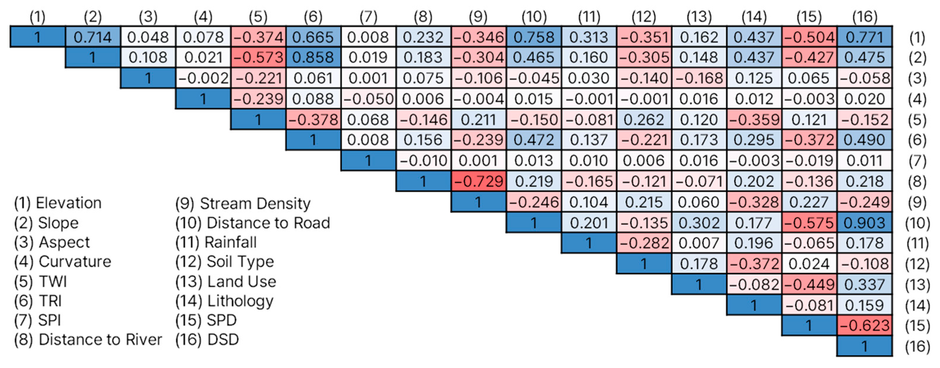
The Pearson’s correlation coefficients between the flood conditioning factors were calculated using IBM SPSS Statistics 26. The results are shown in Figure 4. The coefficients range from −1.0 to 1.0, with values closer to 0 suggesting a weaker correlation.

Figure 4.
The Pearson’s correlation coefficients between the flood conditioning factors considered in this study. Blue and red cells denote positive and negative correlations, respectively.
The multicollinearity analysis (Table 2) showed VIF values ranging from 1.075 to 7.632 and tolerance values from 0.131 to 0.930. The aspect had the lowest VIF and highest tolerance, while DSD had the highest VIF and the lowest tolerance. All of the variables met acceptable thresholds (VIF < 10, Tolerance > 0.1) and were included in the flood susceptibility assessment.
Table 2.
The multicollinearity statistics for the flood conditioning factors considered in this study. All variables met acceptable thresholds (Variance Inflation Factor (VIF) < 10, Tolerance > 0.1) and were included in the analysis.
4.2. Generation of Flood Susceptibility Maps
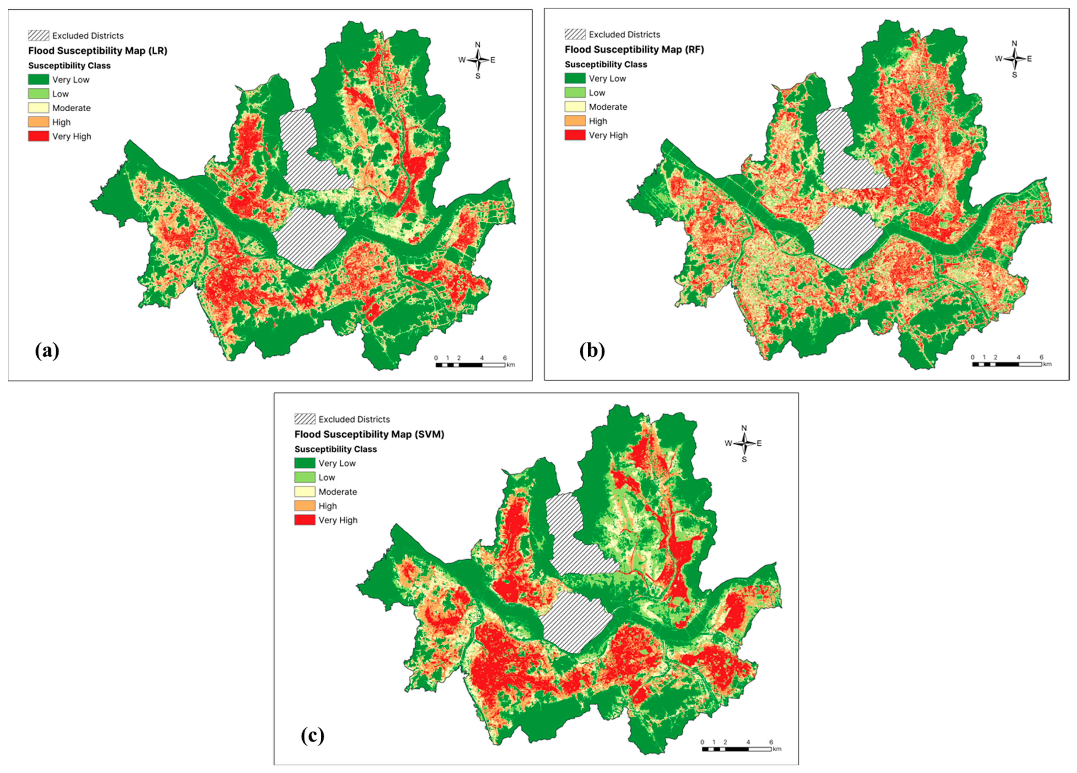
Individual pixels within the study area were assigned values for each of the 16 flood conditioning factors, and were then used as the input parameters to train the three machine learning models. The models were then used to predict the flood susceptibility over the entire study area. Then, the flood susceptibility values were categorized into the following five classes using the Natural Jenks classification in ArcGIS 10.8: very low, low, moderate, high, and very high. The resulting flood susceptibility maps are presented in Figure 5.
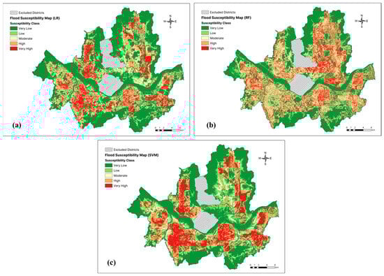
Figure 5.
Flood susceptibility maps produced using each machine learning model: (a) logistic regression (LR), (b) random forest (RF), (c) support vector machines (SVM).
Table 3 presents the percentage distributions of the flood susceptibility classes generated by each model. In the map produced using LR, the majority of the study area was classified as having very low or low flood susceptibility, accounting for 48.68% and 12.23% of the area, respectively. Moderate-susceptibility areas comprise 12.43% of the study area, while high- and very high-susceptibility areas comprise for 12.91% and 13.75%, respectively.
Table 3.
The percentage of the study area attributed to each flood susceptibility class for each machine learning model.
The RF model also categorized most of the study area as having a very low (34.38%) or low (17.46%) flood susceptibility. A total of 15.50% of the study area was classified as moderate-susceptibility, with 15.42% and 17.23% classified as high- and very high-susceptibility, respectively.
Lastly, the SVM model categorized 43.24% and 16.84% of the study area as having very low and low flood susceptibility, respectively. A total of 9.11% of the area was classified as moderate-susceptibility, while 12.73% and 18.08% were classified as high- and very high-susceptibility, respectively.
4.3. Validating the Models
The calculated ROC-AUC, accuracy, F1-score, and kappa metrics are shown in Table 4. The RF model outperformed the SVM and LR models in all four metrics. Therefore, this was chosen as the optimal model for mapping flood susceptibility.
Table 4.
The computed values of four assessment metrics for the three machine learning models. ROC-AUC: Receiver Operating Characteristic (ROC)-area under the ROC curve.
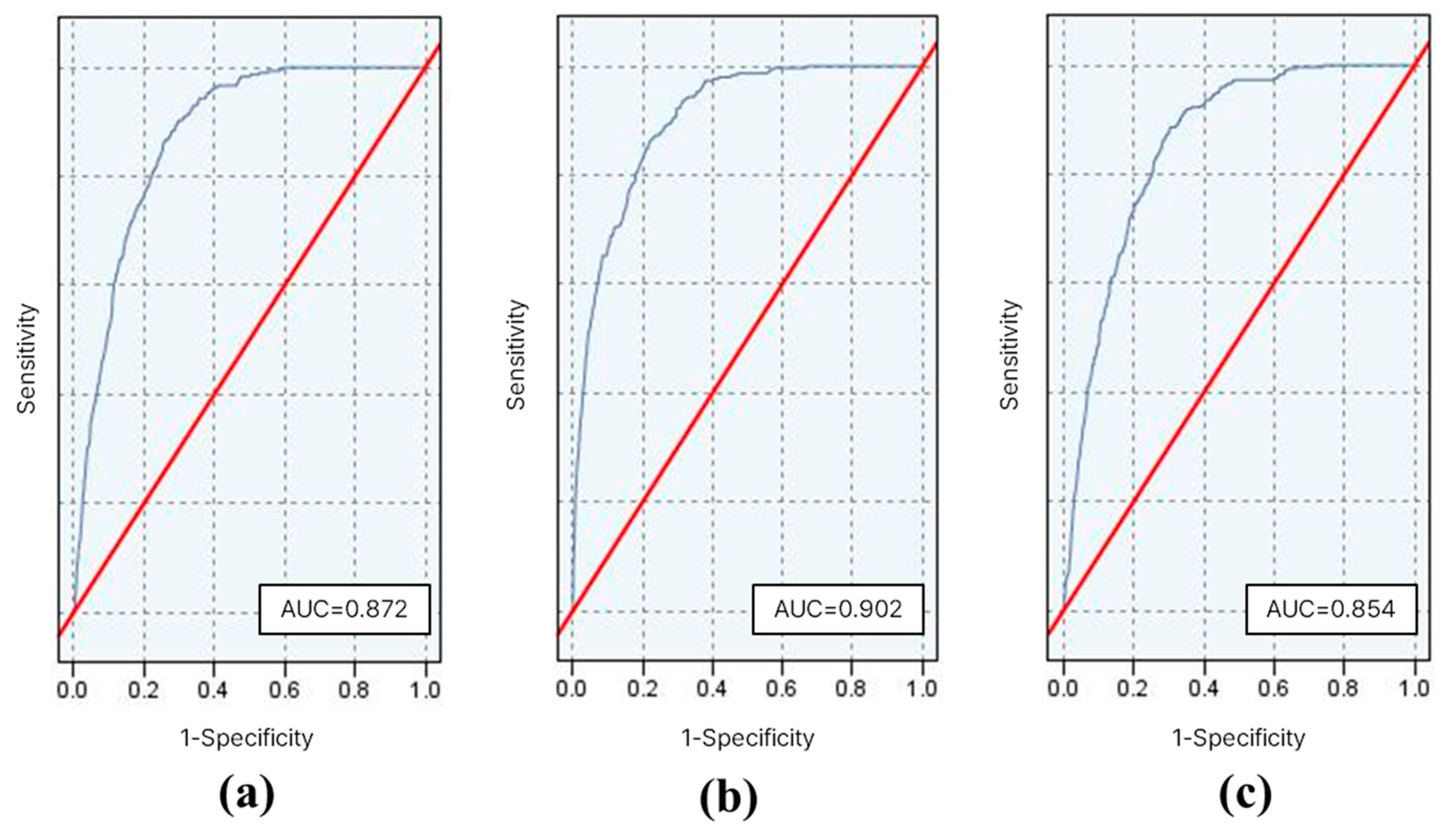
The ROC curves and their corresponding AUC values are shown in Figure 6. The RF model exhibited the highest AUC of 0.902, indicating its ability to distinguish between flood-prone and non-flood-prone areas. The AUC values of the LR and SVM models were 0.872 and 0.854, respectively.

Figure 6.
The Receiver Operating Characteristic (ROC) curve (blue line) and the area under the ROC curve (AUC) for each machine learning model: (a) logistic regression (LR), (b) random forest (RF), (c) support vector machines (SVM). The red line denotes the random classifier.
4.4. Relative Importance and Partial Dependence of Flood Conditioning Factors
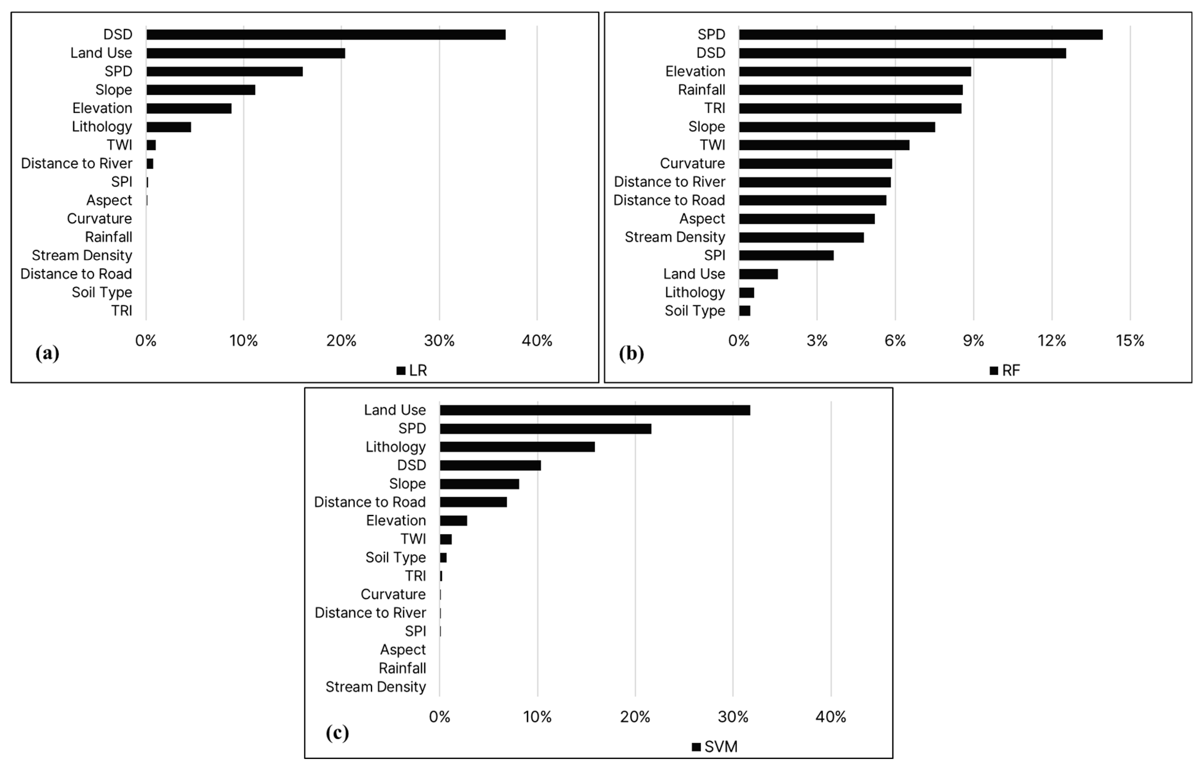
The relative importance of the flood conditioning factors for each model is shown in Figure 7. The results indicate that SPD and DSD are the primary contributing factors to flood susceptibility in Seoul. Conversely, SPI, aspect, stream density, and soil type have a relatively minor influence on flood susceptibility.

Figure 7.
The relative importance of each flood conditioning factor in each model: (a) LR, (b) RF, and (c) SVM.
While the relative importance of the flood conditioning factors varies among the machine learning methods, there is some similarity. Four of the top five flood conditioning factors are consistent between LR and SVM, namely, SPD, DSD, land use, and slope. However, only three of the top five are consistent between the RF and LR models (i.e., SPD, DSD, and elevation), while only two are consistent between the RF and SVM models (i.e., SPD and DSD). This divergence is also reflected in disparities in the prediction maps of each model.
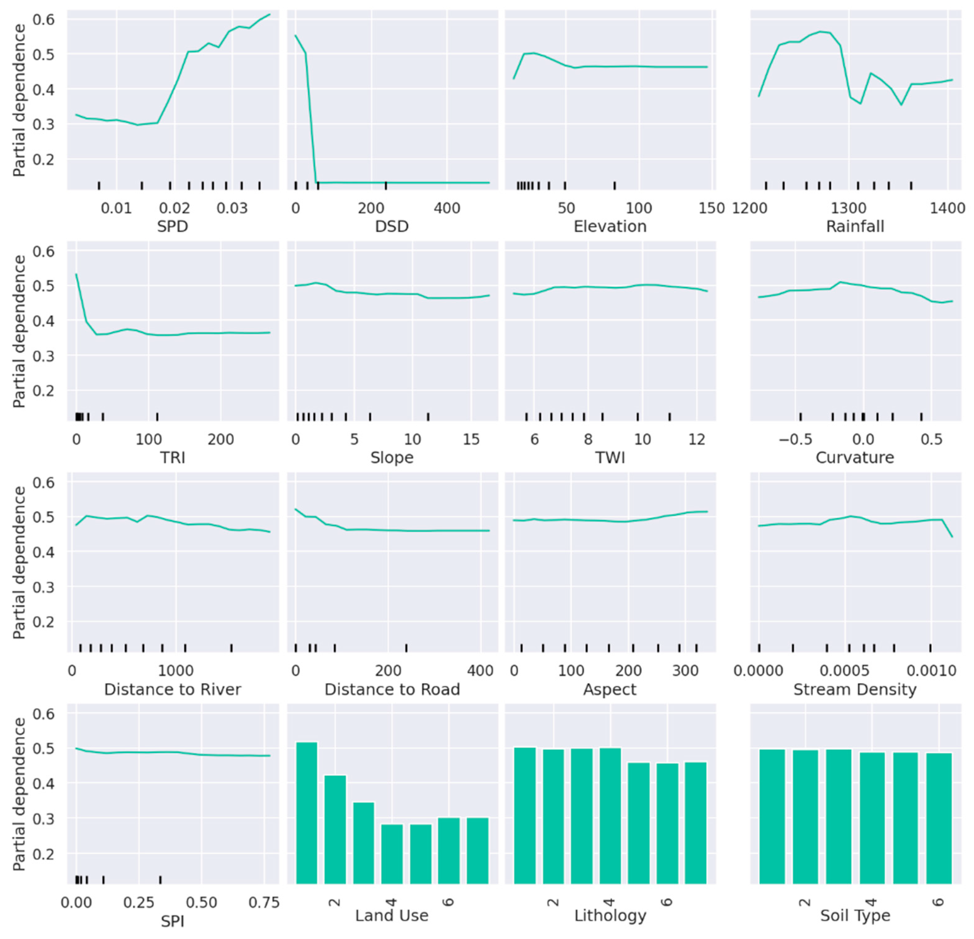
Furthermore, the partial dependencies of the flood conditioning factors were determined for the RF model, as shown in Figure 8. Partial dependence plots (PDPs) are invaluable for interpreting the relationship between dependent variables and each independent variable in a random forest model. The results provide several insights regarding flood occurrence in Seoul: (a) flood occurrence increases significantly with SPD and DSD; (b) elevated areas tend to have lower flood occurrence; and (c) a greater proximity to roads and streams is associated with a higher flood occurrence.
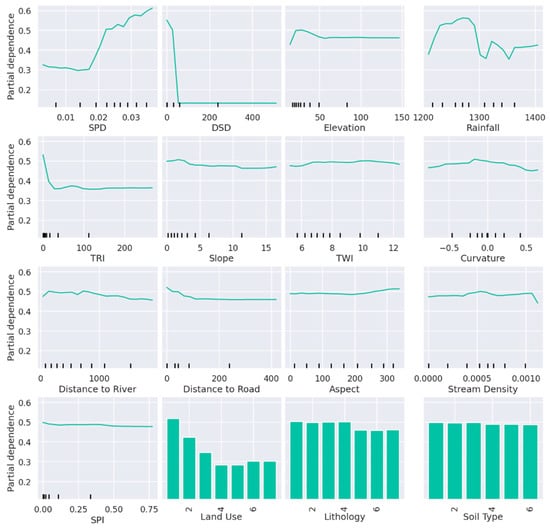
Figure 8.
Partial dependence plots of the flood conditioning factors for the RF model.
4.5. Impact of Drainage-Related Variables
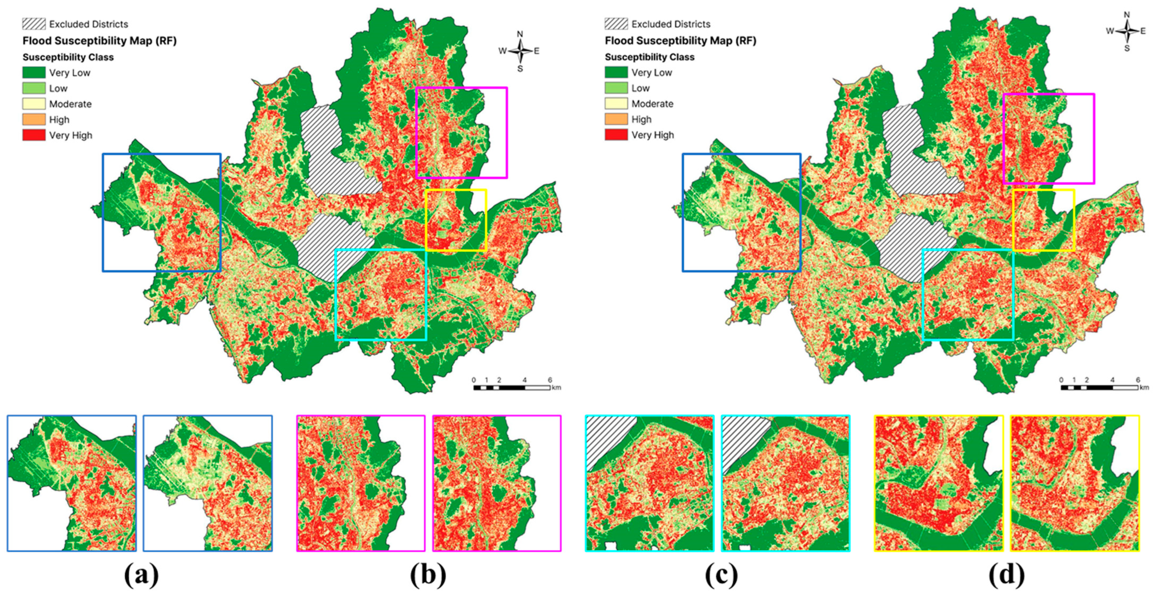
To evaluate the significance of the two drainage-related variables for flood susceptibility in the study area, the optimal model was rerun, while excluding SPD and DSD. Comparing the flood susceptibility maps generated with and without these variables revealed noticeable differences in the susceptibility distribution. As shown in Figure 9b, without drainage-related data, the model tended to overestimate flood risk in the areas that were well drained by sewer systems, leading to a larger area of high-susceptibility zones. In contrast, as shown in Figure 9a, when the drainage-related variables were included, there were more low-susceptibility areas, reflecting the effectiveness of drainage systems in reducing the flood risk in nearby areas by diverting stormwater flow. These observations highlight the crucial importance of incorporating drainage-related factors in urban flood susceptibility mapping.
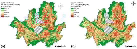
Figure 9.
A comparison of the flood susceptibility maps generated using the RF model: (a) with drainage-related variables, and (b) without drainage-related variables.
Furthermore, when drainage-related variables were included in the flood susceptibility model, areas such as Gangseo-gu (Figure 10a) and Jungnang-gu (Figure 10b) were predicted to have low susceptibility; however, these areas were classified as highly susceptible when these variables were excluded. Conversely, when drainage-related variables were included, the Gangnam-gu (Figure 10c) and Gwangjin-gu (Figure 10d) areas were identified as highly susceptible; however, these areas were predicted to have low susceptibility when these variables were excluded. In the model without drainage-related variables, 45.09% of the study area was classified as low, 18.38% as moderate, and 36.53% as high susceptibility. Meanwhile, the model with drainage-related variables classified 51.84% of the study area as low, 15.50% as moderate, and 32.65% as high susceptibility.
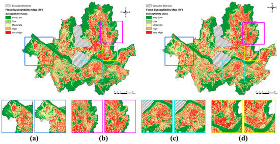
Figure 10.
A comparison of flood susceptibility maps generated with the RF model including drainage-related variables (left) and excluding drainage-related variables (right), highlighting specific areas of Seoul: (a) Gangseo-gu, (b) Jungnang-gu, (c) Gangnam-gu, and (d) Gwangjin-gu.
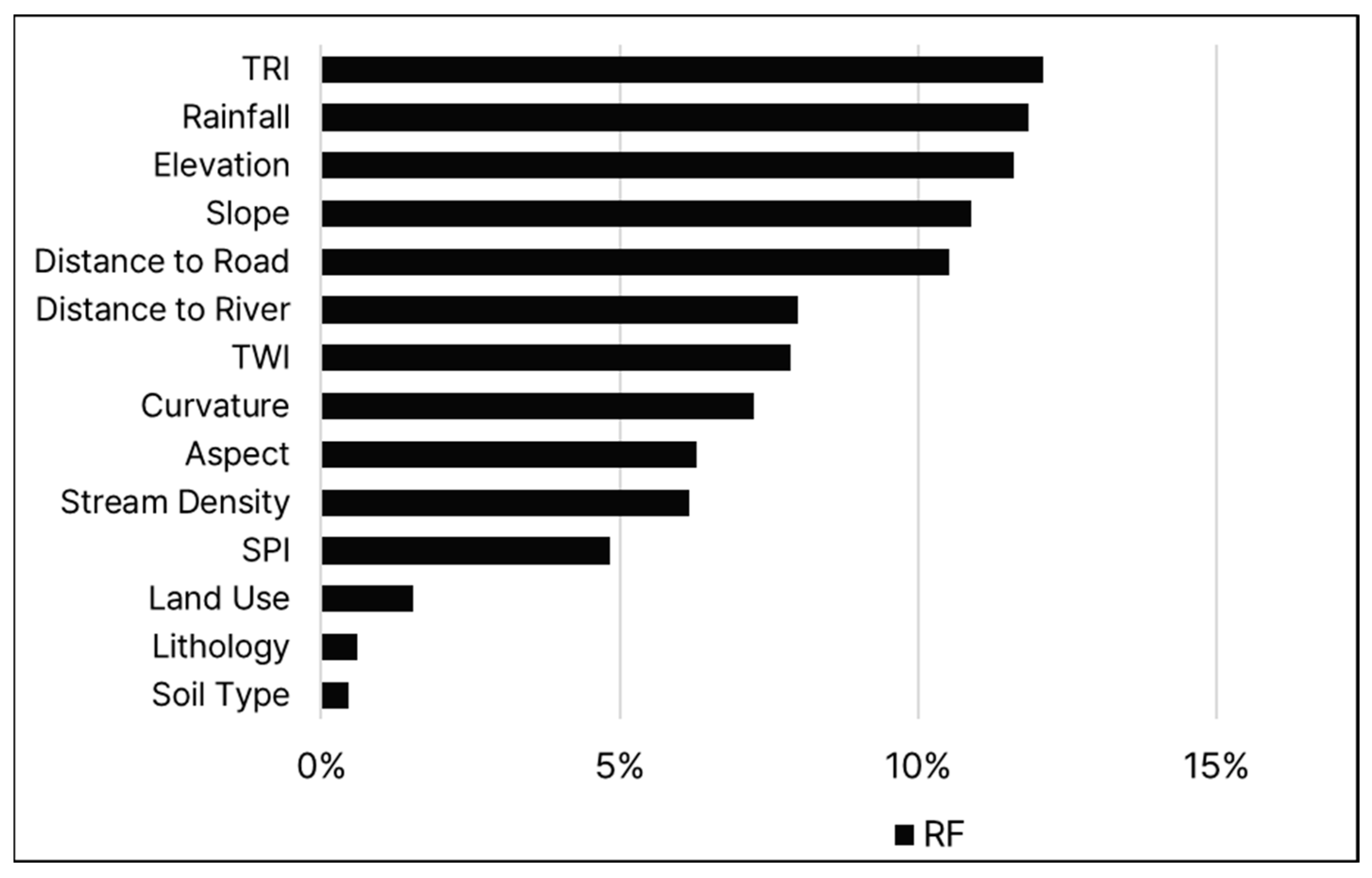
Regarding the relative importance of variables, in the model without drainage-related factors, TRI was found to be the most influential, followed by rainfall, elevation, slope, and distance to a road (Figure 11). Meanwhile, in the model with drainage-related variables, SPD and DSD were the most influential variables, followed by elevation, rainfall, and TRI.

Figure 11.
The relative importance of each variable in the RF model excluding the drainage-related variables.
Additionally, compared to the model that included drainage-related variables, the importance of the factors was more uniform in the model that excluded these variables, with the top five variables each contributing around 11 to 12% to the model. This underscores the significant role of SPD and DSD in urban pluvial flood susceptibility.
Additionally, the evaluation metrics ROC-AUC, accuracy, F1-score, and kappa were calculated for the optimal model without drainage-related variables. The results are presented in Table 5 together with the results for the optimal model including drainage-related variables. Compared to the model without these variables, the model that included drainage-related variables performed better in all metrics, with the accuracy being 7.58% higher and the ROC-AUC 3.80% higher.
Table 5.
The assessment metrics for the RF models with and without drainage-related variables.
5. Discussion
5.1. Flood Susceptibility Maps
The global community faces considerable challenges due to climate change, has led to significant damage and financial losses due to unprecedented meteorological events such as intense typhoons and heavy precipitation. In recent decades, the frequency and severity of floods have significantly increased in South Korea. Using a range of climate change scenarios, Sung et al. [61] showed that the maximum 24 h rainfall in Seoul is expected to increase by approximately 18% in the latter half of the 21st century compared to 2022. This highlights the ongoing impacts of climate change and the need for a more effective approach to managing flood risks. In response, governmental bodies around the world, including South Korea, have created flood risk maps to inform residents about regions at a high risk of severe inundation and facilitate effective evacuation procedures. However, these maps have proven insufficient in accounting for specific variables, such as changes in the built environment [5,62]. For instance, Flores et al. [5] demonstrated that US government-provided maps, such as FEMA’s 100-year flood maps in the U.S., frequently overlook certain flood-prone areas. To address this, they used flood-modeled risk maps to analyze the distribution of flood risks in areas for which FEMA maps were not available. Similarly, Collins et al. [62] used spatial data from Hurricane Harvey in Greater Houston to reveal disparities in flood impacts based on socioeconomic status and race/ethnicity. They found that racial minorities and low-income families experienced more extensive flooding. Therefore, there is a pressing need to develop flood susceptibility maps based on quantitative data.
This study integrated drainage-related data with factors that have been established by empirical research to contribute significantly to flood events within the study area. Furthermore, this work emphasizes the critical importance of the careful selection of explanatory variables and the validation of historical flood occurrences for identifying flood-prone areas.
The flood susceptibility maps generated using the optimal model (RF) indicate that roughly 32% of the study area is susceptible to flooding (i.e., a high or very high risk), with the most vulnerable areas being concentrated near river networks. These susceptible areas are primarily categorized as residential (53.85%), commercial (21.34%), and transportation facilities (16.09%). This result underscores the significant impact of urbanization and land use dynamics on flooding in Seoul. Additionally, the flood susceptibility maps indicate a higher flood risk in southern Seoul, while northern districts have a relatively low risk.
By comparing the generated flood susceptibility maps with flood susceptibility maps of Seoul created in prior studies using similar models, notable differences are apparent. For instance, Lee et al. [6] created a flood susceptibility map of Seoul using an RF model. Compared to the RF-generated map in our study, there are slight differences in the spatial distribution of areas with high and very high flood susceptibility. Specifically, the map of Lee et al. predicts a low susceptibility in northeastern Seoul, whereas the map produced in the present study predicts a high susceptibility in this region due to the presence of streams. These differences are likely due to variations in the input variables employed by each study.
Additionally, similar differences are observed in the LR-based flood susceptibility maps of Lee et al. [7]. This map also predicts a low susceptibility in northeastern Seoul, whereas the LR map produced in the current study predicts a high susceptibility in this region. However, the flood susceptibility map generated using the optimal model (RF) in the present study is generally similar to the one produced by Lei et al. [10] using a CNN.
5.2. Impact of Flood Conditioning Factors
An important finding of this research is the consistent recognition of two drainage-related variables—SPD and DSD—as significant factors influencing flooding in Seoul. Both these variables were ranked among the top five contributing factors to flood susceptibility by all three ML models. This underscores the role of sewer pipes and storm drains in directing water flow, especially during intense rainfall events. No previous research had investigated the effect of these parameters on flood susceptibility in Seoul, and this therefore represents a novel avenue for flood risk analysis.
Furthermore, the results of the optimal model (RF) indicate that elevation, rainfall, and TRI are also crucial predictors of flooding in Seoul. Elevation is a critical determinant of flood risk as low-elevation areas have a lower natural drainage potential. The identification of rainfall as a critical factor was expected as its intensity and volume directly impact the likelihood of flooding. Meanwhile, the TRI quantifies the degree of surface irregularity or roughness, both of which significantly influence flood susceptibility.
A comparative analysis between the flood susceptibility maps of Seoul produced in this study and those of previous studies reveals similarities and differences. For example, Lei et al.’s [10] used neural networks to produce flood susceptibility maps of Seoul and identified TRI, slope, elevation, and TWI as the most crucial flood conditioning factors. Conversely, using an RF model, Lee et al. [6] identified distance to a river, geological characteristics, and elevation as the top three most influential variables in flood occurrence. The identification of elevation and TRI as significant flood conditioning factors in these studies support the results of the present study.
5.3. Model Performance Comparison
This study applied three ML models calibrated with the same flood conditioning factors to the same case study to determine which had the highest predictive accuracy for flood susceptibility. An evaluation using four performance metrics revealed that, although all models performed well, with minor discrepancies in fitting the training dataset, the RF model performed best, followed by the SVM and LR models.
Differences in the relative importance of flood conditioning factors between this and previous studies can be attributed to differences in data sources, modeling methodologies, study area, and flood events considered. This underscores the need for a holistic understanding of the local context and careful consideration of multiple factors when interpreting the relative importance of different variables in flood susceptibility analysis.
Additionally, it was observed that the ML models predicted different flood susceptibility distributions despite exhibiting similar statistical performances. This divergence stems from the different selection procedures and combinations of variables used in each model. For instance, the RF model introduces stochasticity for each variable through random permutation, while SVM attempts to establish an optimal hyperplane discriminating between flood and non-flood classes. Selecting the most suitable model for flood susceptibility mapping is challenging, and regional discrepancies in model performance may introduce uncertainty into spatial predictions. Additionally, it is imperative to consider the impact of future changes in conditions on the accuracy of flood susceptibility maps during their interpretation.
5.4. Study Limitations
Although two flood conditioning factors related to the urban drainage system were considered in this research, it is necessary to incorporate a broader range of drainage-related factors to increase the accuracy of urban pluvial flood modeling. Additionally, this study did not consider issues related to spatial autocorrelation when selecting flooded and non-flooded points as dependent variables. Most ML methods assume that the training and testing datasets follow an independent and identical distribution (IID) [63,64], however, spatial datasets often display spatial autocorrelation, which violates this assumption. Therefore, future research should address spatial autocorrelation when selecting dependent variables to enhance the accuracy of flood susceptibility modeling. Lastly, there has been a recent rise in the use of deep-learning models in flood susceptibility modeling [10]. As a result, future research should apply the flood conditioning factors used in the present study to deep-learning models and compare the results with those of conventional ML models.
6. Conclusions
The primary objective of this research was to evaluate and map urban pluvial flood susceptibility in Seoul, South Korea, using machine-learning techniques and integrating spatial datasets of 16 flood conditioning factors, including drainage-related data. Three machine-learning techniques were used, LR, RF, and SVM. The models effectively demonstrated the relationships between the studied factors and areas that experienced inundation between 2010 and 2022. The resulting flood susceptibility maps were validated and a comparative assessment was performed using four evaluation metrics. The results indicate that the RF model outperformed the other two models, achieving an accuracy of 83.70% and an AUC of 0.902, making it the optimal choice for generating flood susceptibility maps for Seoul. Moreover, the results highlight the significance of the drainage-related variables SPD and DSD as prominent determinants of flood susceptibility. For the optimal model, including these variables increased the accuracy and AUC values by 7.58% and 3.80%, respectively, emphasizing the need to include these variables in urban flood susceptibility modeling.
This research highlights the importance of incorporating drainage-related factors in flood susceptibility models, which represents a significant advancement in understanding the dynamics of pluvial flooding in urban settings. The results underscore the need for comprehensive pluvial flood risk mapping in urban areas, which can inform land-use planning, guide initiatives related to flood insurance, and aid governmental bodies in developing and implementing evacuation strategies.
Nevertheless, there is a need for further research on flood susceptibility using diverse quantitative methodologies, and to obtain more precise data on flood conditioning factors. Future research should focus on integrating high-resolution temporal data, such as real-time rainfall and hydrodynamic models, to enhance flood prediction accuracy. Furthermore, the use of satellite data to monitor the spatial extent of flooding could improve the accuracy and precision of flood predictions. Additionally, to provide a more holistic understanding of flood vulnerability, studies should include socioeconomic variables and drainage-related factors such as the drainage capacity of pipe systems. Continuous refinement of urban flood susceptibility models is critical to addressing the challenges posed by urbanization and climate change.
Author Contributions
Conceptualization, Julieber T. Bersabe and Byong-Woon Jun; methodology, Julieber T. Bersabe and Byong-Woon Jun; software, Julieber T. Bersabe; validation, Julieber T. Bersabe and Byong-Woon Jun; formal analysis, Julieber T. Bersabe; investigation, Julieber T. Bersabe and Byong-Woon Jun; resources, Julieber T. Bersabe; data curation, Julieber T. Bersabe; writing—original draft preparation, Julieber T. Bersabe; writing—review and editing, Julieber T. Bersabe and Byong-Woon Jun; visualization, Julieber T. Bersabe; supervision, Byong-Woon Jun; project administration, Byong-Woon Jun; funding acquisition, Byong-Woon Jun. All authors have read and agreed to the published version of the manuscript.
Funding
This research received no external funding.
Data Availability Statement
The data presented in this study are available on request from the corresponding author due to the confidentiality of sewage network datasets.
Acknowledgments
This research has received partial support from the Global Korea Scholarship (GKS) program through the National Institute for International Education (NIIED). The authors express sincere appreciation to the Seoul Metropolitan Government for supplying important data crucial to this research.
Conflicts of Interest
The authors declare no conflicts of interest.
References
- Bloch, R.; Jha, A.K.; Lamond, J. Cities and flooding: A guide to integrated urban flood risk management for the 21st century; World Bank: Washington DC, USA, 2012; ISBN 978-0-8213-9477-9. [Google Scholar]
- Ha, G.; Jung, J. The Impact of Urbanization and Precipitation on Flood Damages. J. Korea Plan. Assoc. 2017, 52, 237–252. [Google Scholar] [CrossRef]
- Korea Research Institute for Human Settlements. KRIHS Issue Report No. 67; Korea Research Institute for Human Settlements: Sejong, Republic of Korea, 2022. [Google Scholar]
- Park, S.; Kim, J.; Kang, J. Exploring Optimal Deep Tunnel Sewer Systems to Enhance Urban Pluvial Flood Resilience in the Gangnam Region, South Korea. J. Environ. Manag. 2024, 357, 120762. [Google Scholar] [CrossRef]
- Flores, A.B.; Collins, T.W.; Grineski, S.E.; Amodeo, M.; Porter, J.R.; Sampson, C.C.; Wing, O. Federally Overlooked Flood Risk Inequities in Houston, Texas: Novel Insights Based on Dasymetric Mapping and State-of-the-Art Flood Modeling. Ann. Am. Assoc. Geogr. 2023, 113, 240–260. [Google Scholar] [CrossRef]
- Lee, S.; Kim, J.C.; Jung, H.S.; Lee, M.J.; Lee, S. Spatial Prediction of Flood Susceptibility Using Random-Forest and Boosted-Tree Models in Seoul Metropolitan City, Korea. Geomat. Nat. Hazards Risk 2017, 8, 1185–1203. [Google Scholar] [CrossRef]
- Lee, S.; Lee, S.; Lee, M.J.; Jung, H.S. Spatial Assessment of Urban Flood Susceptibility Using Data Mining and Geographic Information System (GIS) Tools. Sustainability 2018, 10, 648. [Google Scholar] [CrossRef]
- Lee, J.Y.; Kim, J.S. Detecting Areas Vulnerable to Flooding Using Hydrological-Topographic Factors and Logistic Regression. Appl. Sci. 2021, 11, 5652. [Google Scholar] [CrossRef]
- Narimani, R.; Jun, C.; Shahzad, S.; Oh, J.; Park, K. Application of a Novel Hybrid Method for Flood Susceptibility Mapping with Satellite Images: A Case Study of Seoul, Korea. Remote Sens. 2021, 13, 2786. [Google Scholar] [CrossRef]
- Lei, X.; Chen, W.; Panahi, M.; Falah, F.; Rahmati, O.; Uuemaa, E.; Kalantari, Z.; Ferreira, C.S.S.; Rezaie, F.; Tiefenbacher, J.P.; et al. Urban Flood Modeling Using Deep-Learning Approaches in Seoul, South Korea. J. Hydrol. 2021, 601, 126684. [Google Scholar] [CrossRef]
- Palla, A.; Colli, M.; Candela, A.; Aronica, G.T.; Lanza, L.G. Pluvial Flooding in Urban Areas: The Role of Surface Drainage Efficiency. J. Flood Risk Manag. 2018, 11, S663–S676. [Google Scholar] [CrossRef]
- Carmin, J.; Dodman, D.; Chu, E.; Carmin, J.; Dodman, D.; Chu, E. Urban Climate Adaptation and Leadership: From Conceptual Understanding to Practical Action Green Growth and Poverty Reduction: Policy Coherence for Pro-Poor Growth; OECD Regional Development Working Papers; OECD Publishing: Paris, France, 2013. [Google Scholar]
- Atta-ur-Rahman; Parvin, G.A.; Shaw, R.; Surjan, A. Cities, Vulnerability, and Climate Change. In Urban Disasters and Resilience in Asia; Butterworth-Heinemann: Oxford, UK, 2016. [Google Scholar]
- Lee, S.; Kim, B.; Choi, H.; Noh, S.J. A Review on Urban Inundation Modeling Research in South Korea: 2001-2022. J. Korea Water Resour. Assoc. 2022, 55, 707–721. [Google Scholar]
- Ha, J.; Kang, J.E. Assessment of Flood-Risk Areas Using Random Forest Techniques: Busan Metropolitan City. Nat. Hazards 2022, 111, 2407–2429. [Google Scholar] [CrossRef]
- Agonafir, C.; Lakhankar, T.; Khanbilvardi, R.; Krakauer, N.; Radell, D.; Devineni, N. A Review of Recent Advances in Urban Flood Research. Water Secur. 2023, 19, 100141. [Google Scholar] [CrossRef]
- Chang, H.; Franczyk, J. Climate Change, Land-Use Change, and Floods: Toward an Integrated Assessment. Geogr. Compass 2008, 2, 1549–1579. [Google Scholar] [CrossRef]
- Seydi, S.T.; Kanani-Sadat, Y.; Hasanlou, M.; Sahraei, R.; Chanussot, J.; Amani, M. Comparison of Machine Learning Algorithms for Flood Susceptibility Mapping. Remote Sens. 2023, 15, 192. [Google Scholar] [CrossRef]
- Wubalem, A.; Tesfaw, G.; Dawit, Z.; Getahun, B.; Mekuria, T.; Jothimani, M. Comparison of Statistical and Analytical Hierarchy Process Methods on Flood Susceptibility Mapping: In a Case Study of the Lake Tana Sub-Basin in Northwestern Ethiopia. Open Geosci. 2021, 13, 1668–1688. [Google Scholar] [CrossRef]
- Solomatine, D.P.; Ostfeld, A. Data-Driven Modelling: Some Past Experiences and New Approaches. J. Hydroinform. 2008, 10, 3–22. [Google Scholar] [CrossRef]
- Fernández, D.S.; Lutz, M.A. Urban Flood Hazard Zoning in Tucumán Province, Argentina, Using GIS and Multicriteria Decision Analysis. Eng. Geol. 2010, 111, 90–98. [Google Scholar] [CrossRef]
- Rahman, M.; Ningsheng, C.; Islam, M.M.; Dewan, A.; Iqbal, J.; Washakh, R.M.A.; Shufeng, T. Flood Susceptibility Assessment in Bangladesh Using Machine Learning and Multi-Criteria Decision Analysis. Earth Syst. Environ. 2019, 3, 585–601. [Google Scholar] [CrossRef]
- Hammami, S.; Zouhri, L.; Souissi, D.; Souei, A.; Zghibi, A.; Marzougui, A.; Dlala, M. Application of the GIS Based Multi-Criteria Decision Analysis and Analytical Hierarchy Process (AHP) in the Flood Susceptibility Mapping (Tunisia). Arab. J. Geosci. 2019, 12, 653. [Google Scholar] [CrossRef]
- Das, S. Flood Susceptibility Mapping of the Western Ghat Coastal Belt Using Multi-Source Geospatial Data and Analytical Hierarchy Process (AHP). Remote Sens. Appl. 2020, 20, 100379. [Google Scholar] [CrossRef]
- Vojtek, M.; Vojteková, J. Flood Susceptibility Mapping on a National Scale in Slovakia Using the Analytical Hierarchy Process. Water 2019, 11, 364. [Google Scholar] [CrossRef]
- Prasad, P.; Loveson, V.J.; Das, B.; Kotha, M. Novel Ensemble Machine Learning Models in Flood Susceptibility Mapping. Geocarto Int. 2022, 37, 1892209. [Google Scholar] [CrossRef]
- Al-Juaidi, A.E.M.; Nassar, A.M.; Al-Juaidi, O.E.M. Evaluation of Flood Susceptibility Mapping Using Logistic Regression and GIS Conditioning Factors. Arab. J. Geosci. 2018, 11, 765. [Google Scholar] [CrossRef]
- Kim, H.I.; Han, K.Y.; Lee, J.Y. Prediction of Urban Flood Extent by LSTM Model and Logistic Regression. KSCE J. Civ. Environ. Eng. Res. 2020, 40, 273–283. [Google Scholar]
- Jung, M.; Kim, J.G.; Uranchimeg, S.; Kwon, H.H. The Probabilistic Estimation of Inundation Region Using a Multiple Logistic Regression Analysis. J. Korea Water Resour. Assoc. 2020, 53, 121–129. [Google Scholar] [CrossRef]
- Abedi, R.; Costache, R.; Shafizadeh-Moghadam, H.; Pham, Q.B. Flash-Flood Susceptibility Mapping Based on XGBoost, Random Forest and Boosted Regression Trees. Geocarto Int. 2022, 37, 5479–5496. [Google Scholar] [CrossRef]
- Chen, W.; Li, Y.; Xue, W.; Shahabi, H.; Li, S.; Hong, H.; Wang, X.; Bian, H.; Zhang, S.; Pradhan, B.; et al. Modeling Flood Susceptibility Using Data-Driven Approaches of Naïve Bayes Tree, Alternating Decision Tree, and Random Forest Methods. Sci. Total Environ. 2020, 701, 134979. [Google Scholar] [CrossRef] [PubMed]
- Mahdizadeh Gharakhanlou, N.; Perez, L. Flood Susceptible Prediction through the Use of Geospatial Variables and Machine Learning Methods. J. Hydrol. 2023, 617, 129121. [Google Scholar] [CrossRef]
- Zhao, G.; Pang, B.; Xu, Z.; Yue, J.; Tu, T. Mapping Flood Susceptibility in Mountainous Areas on a National Scale in China. Sci. Total Environ. 2018, 615, 1133–1142. [Google Scholar] [CrossRef] [PubMed]
- Sahana, M.; Rehman, S.; Sajjad, H.; Hong, H. Exploring Effectiveness of Frequency Ratio and Support Vector Machine Models in Storm Surge Flood Susceptibility Assessment: A Study of Sundarban Biosphere Reserve, India. Catena 2020, 189, 104450. [Google Scholar] [CrossRef]
- Tehrany, M.S.; Pradhan, B.; Jebur, M.N. Flood Susceptibility Mapping Using a Novel Ensemble Weights-of-Evidence and Support Vector Machine Models in GIS. J. Hydrol. 2014, 512, 332–343. [Google Scholar] [CrossRef]
- Tehrany, M.S.; Pradhan, B.; Mansor, S.; Ahmad, N. Flood Susceptibility Assessment Using GIS-Based Support Vector Machine Model with Different Kernel Types. Catena 2015, 125, 91–101. [Google Scholar] [CrossRef]
- Shafapour Tehrany, M.; Shabani, F.; Neamah Jebur, M.; Hong, H.; Chen, W.; Xie, X. GIS-Based Spatial Prediction of Flood Prone Areas Using Standalone Frequency Ratio, Logistic Regression, Weight of Evidence and Their Ensemble Techniques. Geomat. Nat. Hazards Risk 2017, 8, 1538–1561. [Google Scholar] [CrossRef]
- Chen, Y.; Zhang, X.; Yang, K.; Zeng, S.; Hong, A. Modeling Rules of Regional Flash Flood Susceptibility Prediction Using Different Machine Learning Models. Front. Earth Sci. 2023, 11, 1117004. [Google Scholar] [CrossRef]
- Korea Meteorological Association. Changma White Paper; Korea Meteorological Association: Seoul, Republic of Korea, 2022.
- Khojeh, S.; Ataie-Ashtiani, B.; Hosseini, S.M. Effect of DEM Resolution in Flood Modeling: A Case Study of Gorganrood River, Northeastern Iran. Nat. Hazards 2022, 112, 2673–2693. [Google Scholar] [CrossRef]
- Gangani, P.; Mangukiya, N.K.; Mehta, D.J.; Muttil, N.; Rathnayake, U. Evaluating the Efficacy of Different DEMs for Application in Flood Frequency and Risk Mapping of the Indian Coastal River Basin. Climate 2023, 11, 114. [Google Scholar] [CrossRef]
- Seleem, O.; Heistermann, M.; Bronstert, A. Efficient Hazard Assessment for Pluvial Floods in Urban Environments: A Benchmarking Case Study for the City of Berlin, Germany. Water 2021, 13, 2476. [Google Scholar] [CrossRef]
- Seleem, O.; Ayzel, G.; de Souza, A.C.T.; Bronstert, A.; Heistermann, M. Towards Urban Flood Susceptibility Mapping Using Data-Driven Models in Berlin, Germany. Geomat. Nat. Hazards Risk 2022, 13, 1640–1662. [Google Scholar] [CrossRef]
- Sørensen, R.; Zinko, U.; Seibert, J. On the Calculation of the Topographic Wetness Index: Evaluation of Different Methods Based on Field Observations. Hydrol. Earth Syst. Sci. 2006, 10, 101–112. [Google Scholar] [CrossRef]
- Riadi, B.; Barus, B.; Widiatmaka; Yanuar, M.J.P.; Pramudya, B. Identification and Delineation of Areas Flood Hazard Using High Accuracy of DEM Data. IOP Conf. Ser. Earth Environ. Sci. 2018, 149, 012035. [Google Scholar] [CrossRef]
- Grohmann, C.H.; Smith, M.J.; Riccomini, C. Multiscale Analysis of Topographic Surface Roughness in the Midland Valley, Scotland. IEEE Trans. Geosci. Remote 2011, 49, 1200–1213. [Google Scholar] [CrossRef]
- Das, S.; Pardeshi, S.D. Integration of Different Influencing Factors in GIS to Delineate Groundwater Potential Areas Using IF and FR Techniques: A Study of Pravara Basin, Maharashtra, India. Appl. Water Sci. 2018, 8, 197. [Google Scholar] [CrossRef]
- Liu, W.; Song, X.; Huang, F.; Hu, L. Experimental Study on the Disintegration of Granite Residual Soil under the Combined Influence of Wetting–Drying Cycles and Acid Rain. Geomat. Nat. Hazards Risk 2019, 10, 1912–1927. [Google Scholar] [CrossRef]
- Tariq, A.; Yan, J.; Ghaffar, B.; Qin, S.; Mousa, B.G.; Sharifi, A.; Huq, M.E.; Aslam, M. Flash Flood Susceptibility Assessment and Zonation by Integrating Analytic Hierarchy Process and Frequency Ratio Model with Diverse Spatial Data. Water 2022, 14, 3069. [Google Scholar] [CrossRef]
- Pandey, M.; Arora, A.; Arabameri, A.; Costache, R.; Kumar, N.; Mishra, V.N.; Nguyen, H.; Mishra, J.; Siddiqui, M.A.; Ray, Y.; et al. Flood Susceptibility Modeling in a Subtropical Humid Low-Relief Alluvial Plain Environment: Application of Novel Ensemble Machine Learning Approach. Front. Earth Sci. 2021, 9, 659296. [Google Scholar] [CrossRef]
- Edet, A.E.; Okereke, C.S.; Teme, S.C.; Esu, E.O. Application of Remote-Sensing Data to Groundwater Exploration: A Case Study of the Cross River State, Southeastern Nigeria. Hydrogeol. J. 1998, 6, 394–404. [Google Scholar] [CrossRef]
- Falah, F.; Rahmati, O.; Rostami, M.; Ahmadisharaf, E.; Daliakopoulos, I.N.; Pourghasemi, H.R. Artificial Neural Networks for Flood Susceptibility Mapping in Data-Scarce Urban Areas. In Spatial Modeling in GIS and R for Earth and Environmental Sciences; Elsevier: Amsterdam, The Netherlands, 2019. [Google Scholar]
- Kutner, M.H.; Nachtsheim, C.J.; Neter, J. Applied Linear Regression Models, 4th ed.; McGraw-Hill/Irvin: New York, NY, USA, 2004; ISBN 978-0-0723-8691-2. [Google Scholar]
- Breiman, L. Random Forests. Mach. Learn. 2001, 45, 5–32. [Google Scholar] [CrossRef]
- He, Q.; Wang, M.; Liu, K. Rapidly Assessing Earthquake-Induced Landslide Susceptibility on a Global Scale Using Random Forest. Geomorphology 2021, 391, 107889. [Google Scholar] [CrossRef]
- Cortes, C.; Vapnik, V. Support-Vector Networks. Mach. Learn. 1995, 20, 273–297. [Google Scholar] [CrossRef]
- Tien Bui, D.; Pradhan, B.; Lofman, O.; Revhaug, I. Landslide Susceptibility Assessment in Vietnam Using Support Vector Machines, Decision Tree, and Nave Bayes Models. Math. Probl. Eng. 2012, 2012, 974638. [Google Scholar] [CrossRef]
- Hong, H.; Tsangaratos, P.; Ilia, I.; Liu, J.; Zhu, A.X.; Chen, W. Application of Fuzzy Weight of Evidence and Data Mining Techniques in Construction of Flood Susceptibility Map of Poyang County, China. Sci. Total Environ. 2018, 625, 575–588. [Google Scholar] [CrossRef] [PubMed]
- Tharwat, A. Classification Assessment Methods. Appl. Comput. Inform. 2018, 17, 168–192. [Google Scholar] [CrossRef]
- Ferri, C.; Hernández-Orallo, J.; Modroiu, R. An Experimental Comparison of Performance Measures for Classification. Pattern Recognit. Lett. 2009, 30, 27–38. [Google Scholar] [CrossRef]
- Sung, J.H.; Kang, D.H.; Seo, Y.H.; Kim, B.S. Analysis of Extreme Rainfall Characteristics in 2022 and Projection of Extreme Rainfall Based on Climate Change Scenarios. Water 2023, 15, 3986. [Google Scholar] [CrossRef]
- Collins, T.W.; Grineski, S.E.; Chakraborty, J.; Flores, A.B. Environmental Injustice and Hurricane Harvey: A Household-Level Study of Socially Disparate Flood Exposures in Greater Houston, Texas, USA. Environ. Res. 2019, 179, 108772. [Google Scholar] [CrossRef]
- Mahdizadeh Gharakhanlou, N.; Perez, L. Spatial Prediction of Current and Future Flood Susceptibility: Examining the Implications of Changing Climates on Flood Susceptibility Using Machine Learning Models. Entropy 2022, 24, 1630. [Google Scholar] [CrossRef] [PubMed]
- Salazar, J.J.; Garland, L.; Ochoa, J.; Pyrcz, M.J. Fair Train-Test Split in Machine Learning: Mitigating Spatial Autocorrelation for Improved Prediction Accuracy. J. Pet. Sci. Eng. 2022, 209, 109885. [Google Scholar] [CrossRef]


Disclaimer/Publisher’s Note: The statements, opinions and data contained in all publications are solely those of the individual author(s) and contributor(s) and not of MDPI and/or the editor(s). MDPI and/or the editor(s) disclaim responsibility for any injury to people or property resulting from any ideas, methods, instructions or products referred to in the content. |
© 2025 by the authors. Published by MDPI on behalf of the International Society for Photogrammetry and Remote Sensing. Licensee MDPI, Basel, Switzerland. This article is an open access article distributed under the terms and conditions of the Creative Commons Attribution (CC BY) license (https://creativecommons.org/licenses/by/4.0/).