Machine Learning Insights into Supply–Demand Mismatch, Interactions and Driving Mechanisms of Ecosystem Services Across Scales: A Case Study of Xingtai, China

Abstract

To reveal the cross-scale trade-offs and synergies of ecosystem services (ESs) in resource-based cities, this study took Xingtai City, Hebei Province, as a case. Six ESs—water yield (WY), soil retention (SDR), habitat quality (HQ), urban cooling (UC), net primary productivity (NPP), and PM_2.5 removal—were quantified at the 1 km grid, township, and county scales. Using Spearman correlation, geographically weighted regression (GWR), and the XGBoost-SHAP framework, we analyzed the spatiotemporal evolution of the ecosystem service supply–demand ratio (ESDR) from 2000 to 2020 and identified the dominant driving mechanisms. The results indicate the following: (1) The mean ESDR in Xingtai decreased sharply from 0.14 in 2000 to 0.008 in 2020, a decline of 94.3%, showing a pronounced “high in the western mountains–low in the eastern plains” gradient pattern and an increasingly severe supply–demand imbalance. (2) Synergistic relationships dominated among the six ESs, accounting for over 80%. Strong synergies were observed between supply-related services such as WY–SDR and HQ–NPP, with correlation coefficients ranging from 0.65 to 0.88, whereas weak trade-offs (<20%) occurred between UC and PM₂.₅ removal in urbanized areas, which diminished with coarser spatial scales. (3) Population density (Pop), elevation (DEM), cropland proportion (Crop), and vegetation index (NDVI) were identified as the key driving factors, with a combined contribution of 71.4%. NDVI exhibited the strongest positive effect on ecosystem service supply (mean SHAP value = 0.24), while Pop and built-up land proportion showed significant negative effects once exceeding the thresholds of 400 persons/km² and 35%, respectively, indicating nonlinear and threshold-dependent responses. This study quantitatively reveals the spatiotemporal synergy patterns and complex driving mechanisms of ecosystem services in resource-based cities, providing scientific evidence for differentiated ecological restoration and multi-scale governance, and offering essential insights for enhancing regional sustainability.

1. Introduction

Terrestrial ecosystems provide diverse goods and services to human society, playing vital roles in establishing and maintaining environmental conditions and material foundations for human survival and development [1,2]. Varied approaches to natural resource utilization and management induce significant alterations in ecosystem functions, creating trade-off relationships (where enhancement of one service diminishes others) or synergistic interactions (mutual reinforcement) among services such as material production, water provision, soil retention, and carbon sequestration [3,4]. The Millennium Ecosystem Assessment (MA) revealed that accelerating human utilization of certain ecosystem services has led to progressive decline in the provisioning capacity of key services, particularly regulatory and cultural services, severely compromising human well-being and directly threatening ecological security at regional to global scales [5]. Since the onset of the 21st century, China’s rapid industrialization and urbanization have coincided with its GDP exceeding 100 trillion yuan for the first time in 2020. While achieving remarkable economic growth, this process has generated escalating ecological challenges that critically endanger national ecological security [6]. Against this backdrop, quantifying regional ecosystem services and their trade-off/synergy relationships to optimize ecosystem management has emerged as a globally pressing issue.

ESs encompass all utilities or products humans obtain directly or indirectly from ecosystems, categorized into four types: provisioning, supporting, regulating, and cultural services [7]. These services constitute a bridge between natural environmental systems and human societal systems. Ecosystem service supply refers to the services provided by ecosystems for human use, while demand denotes the services actually consumed or utilized by humans [8]. The supply–demand dynamics of ESs effectively indicate whether regional socioeconomic development aligns with natural environmental carrying capacity [9]. Furthermore, complex interrelationships exist among these services, primarily manifested as two fundamental patterns: trade-offs (where increased provision of one service reduces others) [10] and synergies (concurrent enhancement of multiple services) [11]. Consequently, conducting ecosystem service supply–demand assessments to strengthen synergistic effects and mitigate trade-off conflicts has become central to regional ecological restoration and security safeguarding [12]. Thorough investigation of service interactions and their underlying drivers carries profound theoretical and practical significance for enhancing human well-being, strengthening ecological conservation, and promoting high-quality coordinated socioeconomic development [13].

Current research on ES interactions primarily focuses on spatiotemporal distribution patterns [14], driving force analysis [15], scenario simulation [16], scale effects [17], and decision-making applications [18]. Among these, scale effects—which involve dynamic changes in the intensity and direction of ES interactions due to variations in spatiotemporal units—have emerged as a core research challenge [19,20]. While existing studies predominantly employ long-term time series or single-scale frameworks (e.g., provincial or watershed level) to explore ES interactions, comprehensive cross-scale investigations that integrate fine-grained spatial heterogeneity and multi-level socio-ecological feedback remain inadequate [21,22,23]. Recent evidence indicates that trade-offs and synergies often vary significantly across spatial hierarchies due to differences in land use patterns, ecological sensitivity, and human pressure [24]. Therefore, elucidating cross-scale ES relationships and developing multi-level management strategies are essential to enhance human–nature system sustainability in resource-based regions [17,25]. This study, therefore, adopts township-level administrative units for nested multi-scale analysis. Compared with provincial or municipal units, the township scale can preserve spatial integrity while capturing localized socio-ecological interactions because its administrative boundaries often coincide with homogeneous land use mosaics and watershed sub-units [26]. This spatial resolution facilitates the integration of ecological conservation measures with hierarchical planning systems and multi-stakeholder governance mechanisms, thereby bridging macro-level strategies with micro-level implementation needs.

The analysis of driving mechanisms has become a central focus in ES research as the field advances. Current methodologies—including correlation analysis [17], principal component analysis [27,28], structural equation modeling [29], geographically weighted logistic regression (GWLR) [30], geographical detectors [31,32], geographically weighted regression (GWR) [33], geographically weighted binary logistic regression [34], multi-scale geographically weighted regression (MGWR) [35], and random forests [36,37]—have been widely applied to investigate ES driving factors. Nevertheless, these conventional approaches exhibit significant limitations in handling high-dimensional data, capturing nonlinear relationships, and evaluating feature importance. Existing studies often rely on linear analytical frameworks, which may fail to capture the nonlinear feedbacks inherent in complex systems. However, ecosystems themselves can be regarded as complex adaptive systems characterized by nonlinear interactions, dynamic feedback loops, and spatial heterogeneity. In this context, recent years have witnessed machine learning techniques emerging as cutting-edge tools for deciphering ecosystem-driving mechanisms through their superior nonlinear fitting capabilities [38]. Within this context, the XGBoost algorithm has proven particularly valuable for ES research due to its exceptional predictive accuracy, robust nonlinear relationship processing capacity, and precise feature importance ranking [39,40,41]. Compared with the aforementioned traditional methods and other machine learning algorithms, the improvements in this study based on the XGBoost method are mainly reflected in two aspects: first, by adopting the “Boosting integration strategy” that integrates multiple decision trees, the overfitting risk of a single model is effectively reduced, and the fitting stability of the driving relationships of ecological services under the complex landform of Xingtai City is enhanced; second, the SHAP interpretation model is innovatively coupled to break through the interpretability limitation of the XGBoost “black-box model”—it can attribute the model output to the Shapley value of each driving factor. The application of XGBoost may offer novel perspectives and methodologies for better understanding ES driving factors.

Situated in the core area of Beijing–Tianjin–Hebei coordinated development, Xingtai City embodies three distinctive attributes: serving as an ecological barrier along the Taihang Mountains, functioning as a granary for North China, and undergoing resource-based urban transformation. Designated as a key city for regional air pollution control (according to the ‘Key Region Air Pollution Prevention Action Plan’ issued by the Ministry of Ecology and Environment in 2023), Xingtai’s dramatic land use changes and ecological service supply–demand conflicts present an ideal case for examining nonlinear human–environment interactions in resource-dependent cities. This study employs correlation analysis, geographically weighted regression (GWR), and an integrated XGBoost-SHAP model to uncover spatial heterogeneity patterns of ES and their trade-off/synergy relationships (TOSs) across 1 km grid, township, and county scales during 2000–2020. By quantifying demand–supply ratios for six critical services alongside natural–social drivers (e.g., topographic gradients, vegetation coverage changes, and GDP), we reveal nonlinear interaction mechanisms and dominant driving directions of multi-scale ES. The XGBoost-SHAP model enables precise deconstruction of complex trade-off mechanisms driven by coupled natural–social gradients, thereby supporting cross-scale ecological governance decisions and providing scientific foundations for regional administrative management.

2. Materials and Methods

2.1. Study Area Overview

As shown in Figure 1, Xingtai City is situated in southern Hebei Province (113°45′–115°55′ E, 36°45′–37°55′ N), administratively comprising 4 districts, 12 counties, and 2 county-level cities under its jurisdiction. The city spans a total area of 12,457 km², predominantly featuring dry farmland, forested land, and construction land, with a permanent population of 7 million. The territory is divided into two major geomorphological units: mountainous areas in the west and plains in the east. The western mountainous region covers 3545 km² (approximately 28% of the total area), while the eastern plains occupy the remaining 72% without significant transitional zones. Characterized by a typical warm temperate continental monsoon climate, the area receives annual precipitation of 500–600 mm and experiences relative water scarcity. Xingtai possesses abundant natural resources, particularly coal, iron, and mineral deposits, which have crucially supported local industrial infrastructure development and energy security, establishing it as a key resource-based city in Hebei Province and North China. However, the city now faces severe resource depletion and ecological degradation, presenting major challenges for industrial restructuring and ecological restoration.

2.2. ES Supply–Demand Assessment

2.2.1. Quantification of ES Supply–Demand

To quantitatively characterize the spatial distribution and supply–demand features of ESs, this study selected six types of ESs: water yield (WY), soil retention (SDR), habitat quality (HQ), urban cooling (UC), net primary productivity (NPP), and PM_2.5 removal. It should be noted that all demand indicators in this study are estimated using proxies, primarily due to the following practical considerations: First, analyzing long-term time series (2000–2020) and large spatial scales (1 km grid to county/district) requires balancing data availability with temporal consistency (e.g., nighttime light data covering the entire study area with interannual stability). Second, proxy variables must ensure comparability across services (e.g., HQ and NPP) and scales (grid/township/district/county). Third, the relevant literature has validated that similar proxies can effectively reveal spatial trade-offs/synergies in resource-based regions [42]. Corresponding supply and demand indicators were constructed for each, and the estimation methods are presented in

Table 1. Description of model frameworks, input parameters, and supply-demand metrics for six ES (S: supply, D: demand) models.

ESs	Model Process	Parameter Description
WY	S:${\mathrm{S}}_{\mathrm{wy}}=\left[1-{\displaystyle \frac{{\mathrm{A}}_{\left(\mathrm{x}\right)}}{{\mathrm{P}}_{\left(\mathrm{x}\right)}}}\right]\times {\mathrm{P}}_{\left(\mathrm{x}\right)}$	${\mathrm{S}}_{\mathrm{wy}}$ = water production service supply (mm), ${\mathrm{A}}_{\left(\mathrm{x}\right)}$ = actual annual evapotranspiration (mm), ${\mathrm{P}}_{\left(\mathrm{x}\right)}$ = annual precipitation for raster cell x (mm) [43].
	D:${\mathrm{D}}_{\mathrm{wy}}={\mathrm{W}}_{\mathrm{dom}} +{ \mathrm{W}}_{\mathrm{agr}} +{ \mathrm{W}}_{\mathrm{eco}} +{ \mathrm{W}}_{\mathrm{oth}}$	${\mathrm{D}}_{\mathrm{wy}}$ = the demand for water production services. ${\mathrm{W}}_{\mathrm{dom}}$, ${\mathrm{W}}_{\mathrm{agr}}$, ${\mathrm{W}}_{\mathrm{eco}}$, ${\mathrm{W}}_{\mathrm{oth}}$ represent industrial and domestic water use, agricultural water use, ecological water use, and other water use.
SDR	S:$\mathrm{SD}=\mathrm{RKLS}-\mathrm{USLE}$ $\mathrm{USLE}=\mathrm{R}\times \mathrm{K}\times \mathrm{LS}\times \mathrm{C}\times \mathrm{P}$ $\mathrm{RLKS}=\mathrm{R}\times \mathrm{K}\times \mathrm{LS}$	SD = soil retention demand, RKLS = potential soil erosion, USLE = actual soil erosion, R = rainfall erosivity factor, K = soil erodibility factor, LS = topographic factor (slope length/steepness), C = vegetation management factor, P = anthropogenic measures factor.
	D:$\mathrm{USLE}=\mathrm{R}\times \mathrm{K}\times \mathrm{LS}\times \mathrm{C}\times \mathrm{P}$
HQ	S:${\mathrm{S}}_{\mathrm{HQ}}={\mathrm{H}}_{\mathrm{j}}\left[1-\left({\displaystyle \frac{{\mathrm{D}}_{{\mathrm{xj}}^{\mathrm{z}}}}{{\mathrm{D}}_{{\mathrm{xj}}^{\mathrm{z}}} +{ \mathrm{k}}^{\mathrm{z}}}}\right)\right]$	${\mathrm{S}}_{\mathrm{HQ}}$ = the level of provision of habitat quality services, Dxj = the level of stress experienced by raster x in land use type j, ${\mathrm{H}}_{\mathrm{j}}$ = the habitat suitability of land use type j k = a scaling constant, z = a normalization constant [44].
	D:${\mathrm{D}}_{\mathrm{HQ}}={\displaystyle \frac{{\sum }_{\mathrm{k}=1}^{\mathrm{M}}{\mathrm{S}}_{\mathrm{HQ}}}{\mathrm{S}}}$ ${\mathrm{D}}_{\mathrm{HQ}}=\left\{\begin{array}{c}{\mathrm{D}}_{\mathrm{HQ}}-{\mathrm{S}}_{\mathrm{HQ}} {\mathrm{S}}_{\mathrm{HQ}}<{\mathrm{D}}_{\mathrm{HQ}}\\ 0 { \mathrm{S}}_{\mathrm{HQ}}\ge {\mathrm{D}}_{\mathrm{HQ}}\end{array}\right.$	${\mathrm{D}}_{\mathrm{HQ}}$ = the habitat quality requirement standard S = the size of the study area (km2).
UC	S$:{\mathrm{HM}}_{\mathrm{i}}=\left\{\begin{array}{c}C{\mathrm{C}}_{\mathrm{i}}\left({\mathrm{CC}}_{\mathrm{i}}>{\mathrm{CC}}_{{\mathrm{park}}_{\mathrm{i}}}{\mathrm{or} \mathrm{GA}}_{\mathrm{i}}<2\mathrm{ha}\right)\\ C{\mathrm{C}}_{{\mathrm{park}}_{\mathrm{i}}}\left(Other situations.\right)\end{array}\right.$ ${\mathrm{CC}}_{\mathrm{i}}=0.6\times \mathrm{shade} + 0.2\times \mathrm{albedo} + 0.2\times \mathrm{ETI}$ ${\mathrm{CC}}_{{\mathrm{park}}_{\mathrm{i}}}={\displaystyle {\displaystyle \sum }_{\mathrm{j}\in \mathrm{dradiusfromi}}}{\mathrm{g}}_{\mathrm{j}}\times {\mathrm{CC}}_{\mathrm{j}}\times {\mathrm{e}}^{{\displaystyle \frac{-{\mathrm{d}}_{\mathrm{i},\mathrm{j}}}{{\mathrm{d}}_{\mathrm{cool}}}}}$	HMi = the supply of urban cooling services on image i CCi = the cooling capacity index, shadowing, evapotranspiration and albedo. CCparki = the distance-weighted average of the CC values for the greenfield dcool = the effective greenfield cooling distance.
	$\begin{array}{l}\mathrm{D}:{\mathrm{D}}_{\mathrm{HM}}=({\mathrm{P}}_{\mathrm{density}}\times \max {\mathrm{P}}_{\mathrm{density}}^{-1}\times 0.7 +\\ { \mathrm{P}}_{65+}\times \max {\mathrm{P}}_{65+}^{-1}\times 0.3)\times \mathrm{T}\end{array}$	${\mathrm{D}}_{\mathrm{HM}}$ = the demand for urban cooling, ${\mathrm{P}}_{\mathrm{density}}$ = the population density of the administrative unit, ${\mathrm{P}}_{65+}$ = the percentage of the population over 65 years of age in the administrative unit, T = the mean value of the inversion temperature.
PM2.5	S:${\mathrm{P}}_{\mathrm{pm}2.5}=\mathrm{F}\times \mathrm{LAI}\times \mathrm{T}\times 0.5\times \mathrm{V}\left(\mathrm{x}\right)$ $\mathrm{F}={\mathrm{V}}_{\mathrm{pm}2.5}\times {\mathrm{C}}_{\mathrm{pm}2.5}$ $\mathrm{V}\left(\mathrm{x}\right)=\mathrm{C}\left(\mathrm{x}\right)\times \mathrm{H}$	${\mathrm{P}}_{\mathrm{pm}2.5}$ = Annual PM2.5 Deposition, F = PM2.5 Deposition Flux LAI = Annual Leaf Area Index, ${\mathrm{V}}_{\mathrm{pm}2.5}$ = PM2.5 Deposition Velocity ${\mathrm{C}}_{\mathrm{pm}2.5}$ = Annual PM2.5 Concentration, V(x) = Air Purification Volume (grid x) C(x) = Grid Area, H = PM2.5 Distribution Height.
	D:${\mathrm{PD}}_{\mathrm{pm}2.5}=\left({\mathrm{C}}_{\mathrm{pm}2.5}-{\mathrm{PB}}_{\mathrm{pm}2.5}\right)\times \mathrm{T}\times \mathrm{V}\left(\mathrm{x}\right)$	${\mathrm{PD}}_{\mathrm{pm}2.5}$ = Required PM2.5 Reduction, ${\mathrm{C}}_{\mathrm{pm}2.5}$ = Annual PM2.5 Concentration ${\mathrm{PB}}_{\mathrm{pm}2.5}$= PM2.5 “Excellent” Standard (35 μg/m3).
NPP	S:$\mathrm{NPP}\left(\mathrm{x},\mathrm{t}\right)=\mathrm{APAR}\left(\mathrm{x},\mathrm{t}\right)\times \mathsf{\epsilon }\left(\mathrm{x},\mathrm{t}\right)$ $\mathrm{APAR}\left(\mathrm{x},\mathrm{t}\right)=\mathrm{SOL}\left(\mathrm{x},\mathrm{t}\right)\times 0.5\times \mathrm{FPAR}\left(\mathrm{x},\mathrm{t}\right)$ $\mathsf{\epsilon }\left(\mathrm{x},\mathrm{t}\right)={\mathrm{T}}_{\mathsf{\epsilon }1}\left(\mathrm{x},\mathrm{t}\right)\times {\mathrm{T}}_{\mathsf{\epsilon }2}\left(\mathrm{x},\mathrm{t}\right)\times {\mathrm{W}}_{\mathsf{\epsilon }}\left(\mathrm{x},\mathrm{t}\right)\times {\mathsf{\epsilon }}_{\max }$	NPP(x,t) = Net Primary Productivity, APAR(x,t) = Absorbed Photosynthetically Active Radiation, ε(x,t) = Actual Light Use Efficiency, SOL(x,t) = Total Solar Radiation, FPAR(x,t) = Fraction of Absorbed PAR, Tε1(x,t), Tε2(x,t) = Temperature Stress Coefficients, Wε(x,t) = Water Stress Coefficient, εmax = Maximum Light Use Efficiency.
	D:$\mathrm{CD}={\displaystyle \frac{{\mathrm{DN}}_{\mathrm{x}}}{{\mathrm{DN}}_{\mathrm{sum}}}}\times \mathrm{C}$	CD = Carbon Sequestration Demand, ${\mathrm{DN}}_{\mathrm{x}}$ = Nighttime Light Value (pixel x) ${\mathrm{DN}}_{\mathrm{sum}}$ = Total Regional Nighttime Light Value, C = Total Carbon Emissions.

.

2.2.2. Ecosystem Service Supply-Demand Ratio

Imbalance between ES supply and demand may lead to suboptimal resource utilization. This study integrates ES supply and demand metrics through the Ecosystem Service Supply and Demand Ratio (ESDR) to evaluate the equilibrium status of four ESs within the study area, thereby identifying potential supply-demand conflicts.

$$ESDR={\displaystyle \frac{S-D}{\left(S_{max}+D_{max}\right)/2}}$$

(1)

where: ESDR represents the supply-demand ratio of ES within the study unit; S denotes the actual supply of a given ES; D indicates the actual demand for a given ES; S_max is the maximum value of ES supply; D_max is the maximum value of ES demand.

2.3. Multi-Scale Analysis of Trade-Off/Synergy Relationships

2.3.1. Spearman Correlation Analysis

This study initially employs Spearman’s correlation coefficient (R) and significance (p-value) to analyze trade-off/synergy relationships among ESs in Xingtai City (2000–2020) from a global perspective, with visualization conducted using Origin 2022 software. To enhance analytical precision, three evaluation scales were adopted considering both research scope and data volume: county-level, township-level, and 1 km grid scales [45].

2.3.2. Geographically Weighted Regression (GWR) Model

The geographically weighted regression (GWR) model was applied to examine local-scale trade-off/synergy relationships among ESs at each spatial location, addressing spatial non-stationarity and revealing spatial heterogeneity in these relationships. Positive regression coefficients indicate spatial synergies, while negative coefficients denote spatial trade-offs. The analysis was implemented using the “GWmodel” package in R4.3.2.

$$y_i={\mathsf{\beta }}_0\left(u_i,v_i\right)+{\displaystyle {\displaystyle \sum }_{k=1}^p}{\mathsf{\beta }}_k\left(u_i,v_i\right)x_{jk}+{ \mathsf{\epsilon }}_i$$

(2)

where: $y_i$ is the dependent variable;${\beta }_0\left(u_i,v_i\right)$ represents the intercept at point $i$; $\left(u_i,v_i\right)$ denotes the spatial coordinates of point $i$; $p$ indicates the number of independent variables; ${\beta }_k\left(u_i,v_i\right)$ stands for the regression coefficient; $x_{jk}$ refers to the independent variable; ${\epsilon }_i$ is the error term. Positive regression coefficients indicate spatial synergies, while negative coefficients represent spatial trade-offs. This analysis was implemented using the “GWmodel” package in R version 4.3.2.

2.4. Driving Factor Analysis

2.4.1. Driver Selection

Existing research demonstrates that ES supply–demand relationships are influenced by multidimensional factors. Based on a comprehensive literature review and data availability, eleven indicators were selected to represent the key natural, landscape, and socioeconomic dimensions. Natural condition variables, including precipitation (Pre), temperature (Tem), NDVI, and elevation (DEM), determine the ecological and hydrological basis of ES supply. Landscape composition factors, such as the proportion of cropland (Crop), forest (Forest), and urban land (Urban), reflect the spatial structure and land-use configuration that mediate ecological processes and human disturbances. Socioeconomic variables—population density (Pop), nighttime light intensity (NL), GDP, and human footprint (HF)—capture anthropogenic intensity and economic development levels, which are closely related to ES demand.

These eleven drivers were identified through reference to previous ES studies and adapted to the context of resource-based cities such as Xingtai [46,47]. To ensure model reliability, multicollinearity among all driving factors was examined using the Variance Inflation Factor (VIF) test conducted in SPSS 26.0 software through a stepwise regression method. The results showed that the average VIF values were 1.82 for natural factors (DEM, NDVI, Pre, Tem), 2.15 for landscape composition (Crop, Forest, Urban), and 3.07 for socioeconomic variables (Pop, NL, GDP, HF). All VIF values were below the critical threshold of 5, indicating that no severe multicollinearity existed among the explanatory variables, and all could be retained for the subsequent modeling analysis.

2.4.2. XGBoost Model and SHAP Interpretation

The XGBoost model coupled with SHAP analysis quantifies the effects of 11 environmental and socioeconomic factors.

XGBoost is an ensemble learning algorithm that enhances model generalizability through decision tree integration, outperforming traditional methods in both performance and robustness.

$$L\left(\varphi \right)={{\displaystyle \sum }}_{i}l\left(y_i,\widehat{y_i}\right)+{{\displaystyle \sum }}_k\Omega \left(f_k\right)$$

(3)

where $i$ denotes the $i$-th sample; $k$ represents the $k$-th tree; $\widehat{y_i}$ is the predicted value for sample x_i; $\Omega \left(f_k\right)$ denotes the regularization term; ${{\displaystyle \sum }}_k\Omega \left(f_k\right)$ quantifies the complexity of $k$ trees.

The SHAP interpreter attributes output values to each feature’s Shapley value, thereby evaluating individual drivers’ contributions to final outputs.

$$g\left(z^{\prime }\right)={\varphi }_0+{{\displaystyle \sum }}_{j=1}^M{\varphi }_j{z}_j^{\prime }$$

(4)

where $M$ is the number of driving factors; z_j indicates the presence (1) or absence (0) of the corresponding factor; φ_j represents the attribution value of each driver; φ₀ is a constant.

2.4.3. Model Evaluation

For the XGBoost model, hyperparameter tuning was conducted using the GridSearchCV algorithm combined with 5-fold cross-validation to prevent overfitting and enhance generalization ability. The parameters optimized included the learning rate (learning_rate), tree depth (max_depth), number of trees (n_estimators), subsampling rate (subsample), and column sampling rate (colsample_bytree). The optimal parameter ranges were determined as follows:

learning_rate = 0.05–0.15, max_depth = 4–8, n_estimators = 200–500, subsample = 0.8–1.0, and colsample_bytree = 0.7–1.0.

Model performance was evaluated using multiple indicators, including the coefficient of determination (R²), root mean square error (RMSE), and mean absolute error (MAE), to comprehensively assess model stability and predictive accuracy. The final optimized model achieved stable performance across all ESs, ensuring the robustness of the subsequent SHAP interpretation.

2.4.4. Restricted Cubic Splines

Restricted cubic splines (RCS) fit nonlinear relationships between independent and dependent variables via piecewise polynomials. Applying RCS to drivers’ SHAP values precisely captures complex nonlinear interactions with ESDR. The analysis was implemented using Python 3.13’s “scikit-learn” library (version 1.5.1).

2.5. Data Sources

This study integrated meteorological, remote sensing, and statistical data (

Table 2. Data descriptions and sources.

Data Type	Resolution	Data Source
Land Use	30 m	Resource and Environment Science Data Platform (resdc.cn, accessed on 1 November 2025)
Elevation (DEM)	30 m	Geospatial Data Cloud “Global 30 m SRTM DEM” (http://www.gis5g.com, accessed on 1 November 2025)
Soil Data	1 km	Harmonized World Soil Database (HWSD) v1.2
Precipitation and Evapotranspiration	1 km	National Earth System Science Data Center (geodata.cn, accessed on 1 November 2025)
Temperature	1 km	Geospatial Data Cloud
Land Surface Temperature	1 km	Resource and Environment Science Data Platform
Nighttime Light	1 km	Earth Observation Group, Payne Institute (mines.edu, accessed on 1 November 2025)
Population Density	1 km	LandScan Global 1 km Population Grid
GDP and Energy Consumption	-	National Bureau of Statistics, China Energy Statistical Yearbook
Annual Mean Leaf Area Index (LAI)	1 km	Geospatial Data Cloud “China 1 km Monthly LAI Dataset (2000–2022)” (http://www.gis5g.com, accessed on 1 November 2025)
PM2.5	1 km	National Tibetan Plateau Data Center “High-resolution PM2.5 Dataset (2000–2023)” (tpdc.ac.cn, accessed on 1 November 2025)
Population Age Structure and Water Consumption	County-level	Statistical Yearbooks, Water Resources Bulletins

). All environmental datasets underwent interpolation and spatial analysis to ensure consistency and accuracy, standardized to WGS_1984_UTM_Zone_49N projection using ArcGIS 10.8 software.

3. Results

3.1. Spatiotemporal Variations in ES Supply and Demand

3.1.1. Spatiotemporal Characteristics of ES Supply

The spatial and temporal pattern of ES supply in Xingtai City from 2000 to 2020 exhibited a pronounced west-to-east gradient, transitioning from mountainous to plain areas (Figure 2). Overall, mountainous areas consistently served as high-value zones for ES supply, while plains and urbanized areas showed relatively low supply capacity. The western Taihang Mountain region was characterized by high values of water yield and soil retention services, with a water yield peak of 579 mm (in 2000), strongly associated with high-altitude terrain and forest coverage. Soil retention service peaked at 169.486 t/pixel and was concentrated in hilly areas with slopes greater than 15°. In contrast, the eastern plains were dominated by persistently low soil retention values. Habitat quality showed a binary spatial structure, with high values in the western mountains and low values in the transitional zones between urban and agricultural lands in the east. Low-value zones of urban cooling service (0.08) were clustered in bands across the eastern plains, closely aligned with the spatial extent of built-up areas and surface temperature anomalies. High values of PM_2.5 removal service (269.522 g/m²) were mainly located in western forest belts, while low values (21.2706 g/m²) were found in eastern industrial clusters. Carbon sequestration service (NPP) displayed spatial differentiation, with high values in western forests (5426 kgC/m²) and secondary peaks in eastern farmlands. Areas with zero NPP expanded along transport networks and urban fringes, increasing from 6.3% in 2000 to 14.1% in 2020, mirroring the encroachment of built-up land into ecological space. Temporally, the area of high water yield (>500 mm) remained stable between 2000 and 2010, then shrank by 12.3% after 2010. The spatial center of high NPP areas shifted westward from 2010 to 2020. The low-value zones of urban cooling service (<0.2) expanded from 7.4% of the study area in 2000 to 20.1% in 2020, while low-value zones of PM_2.5 removal service (<50 g/m²) increased from 9.8% to 21.3% over the same period. The proportion of high-value soil retention areas fluctuated by less than 3% from 2000 to 2020, and high-value habitat quality zones remained stable.

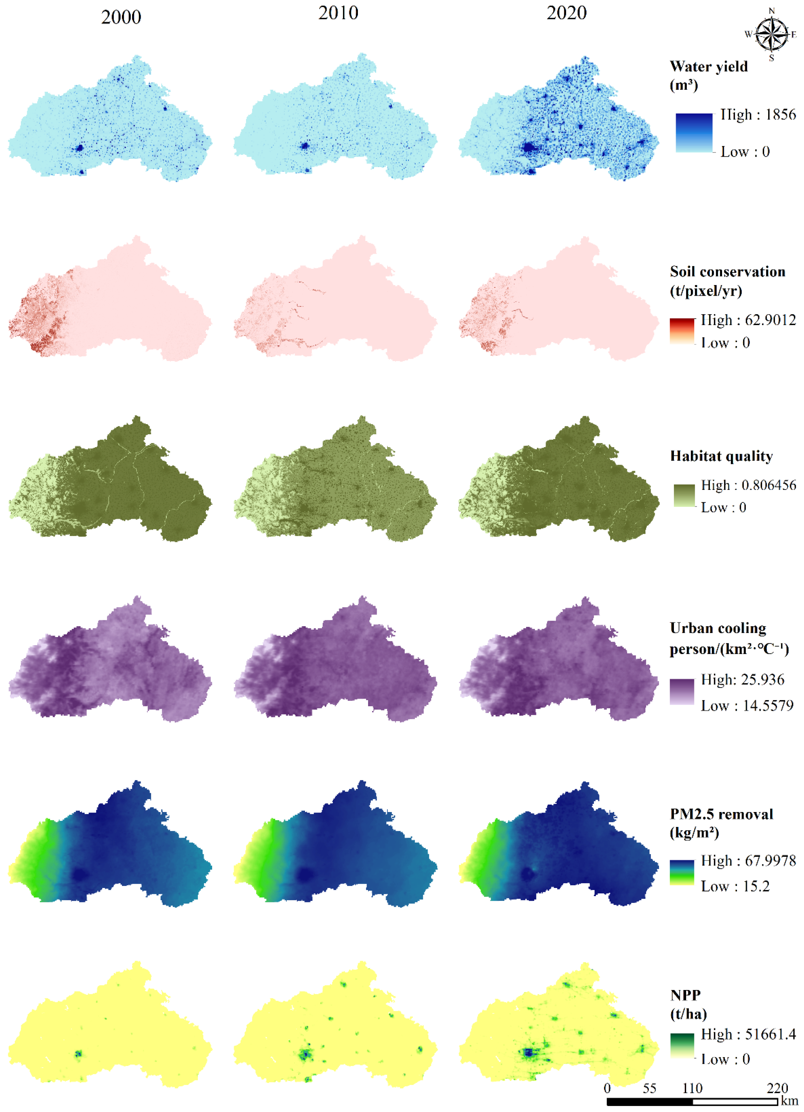
3.1.2. Spatiotemporal Characteristics of ES Demand

As shown in Figure 3, the spatiotemporal pattern of ES demand in Xingtai City from 2000 to 2020 also displayed a significant west-to-east spatial gradient, with an evident expansion trend of high-demand zones driven by urbanization. Spatially, areas with high demand for water yield, urban cooling, PM_2.5 removal, and carbon sequestration services were concentrated in the urbanized eastern plains, closely aligned with the expansion trajectory of built-up land. Low-demand zones remained stable in the mountainous west, constrained by topography and vegetation cover. High-demand zones for soil retention service (>62.9 t/pixel/yr) were located in hilly areas prone to soil erosion, and their extent slightly declined with agricultural intensification. High-demand zones for habitat quality (>0.8) spread along the urban–agricultural transition zones. Notably, demand for urban cooling and PM_2.5 removal services exhibited a prominent spatial clustering pattern, with high-demand zones radiating from urban cores and transport networks. Meanwhile, the spatial compression of habitat quality demand intensified with ongoing urban expansion. Temporally, the demand intensity in urbanized eastern areas increased continuously from 2000 to 2020. The area of high demand for urban cooling and PM_2.5 removal services expanded by 1.8 and 1.5 times, respectively, with peak values rising to 27.1 person/(km²·°C⁻¹) and 70.5 kg/m². High-demand zones for carbon sequestration services gradually shifted toward urban fringes due to farmland intensification. The spatial configuration of low-demand zones in the western mountains remained stable, indicating a strong anchoring effect of natural background conditions on demand regulation.

3.1.3. Spatiotemporal Characteristics of the ES Supply–Demand Ratio

As shown in Figure 4, the supply–demand ratios of six ESs in Xingtai City generally exhibited a spatial gradient of “high in the western mountains, low in the eastern plains,” closely aligned with topography, vegetation coverage, and human activity intensity. From 2000 to 2020, high-value zones of naturally dominated services slightly shrank, while the spatial clustering of low-value zones related to urbanization became more pronounced. The water yield supply–demand ratio maintained a high of 0.30 and a low of −1.80 over the two decades, highlighting the significant contrast between water conservation zones and irrigated agricultural areas. The soil retention supply–demand ratio remained stable at a high of 1.74, mainly in mountain areas with dense vegetation, and a low of −0.04 in intensively cultivated plains. The habitat quality supply–demand ratio ranged from 1.10 to −0.89, reflecting sharp differences between ecological conservation zones and degraded regions, with slight fluctuations in low-value zones due to urban expansion. The urban cooling service supply–demand ratio had a high of 1.00 and a low of −0.89, with low-value zones becoming increasingly clustered though their extent changed little. The PM_2.5 removal service supply–demand ratio ranged from a high of 1.65 to a low of −0.78, with low-value zones strongly overlapping industrial hubs. For carbon sequestration (NPP), the supply–demand ratio peaked at only 0.004 but dropped as low as −1.98, revealing stark contrasts in carbon sink capacity between forests/farmlands and built-up areas. Overall, these extreme mismatches in supply–demand ratios underscore the growing spatial decoupling between ES functions and human demands.

3.2. Trade-Offs and Synergies Among ESDR

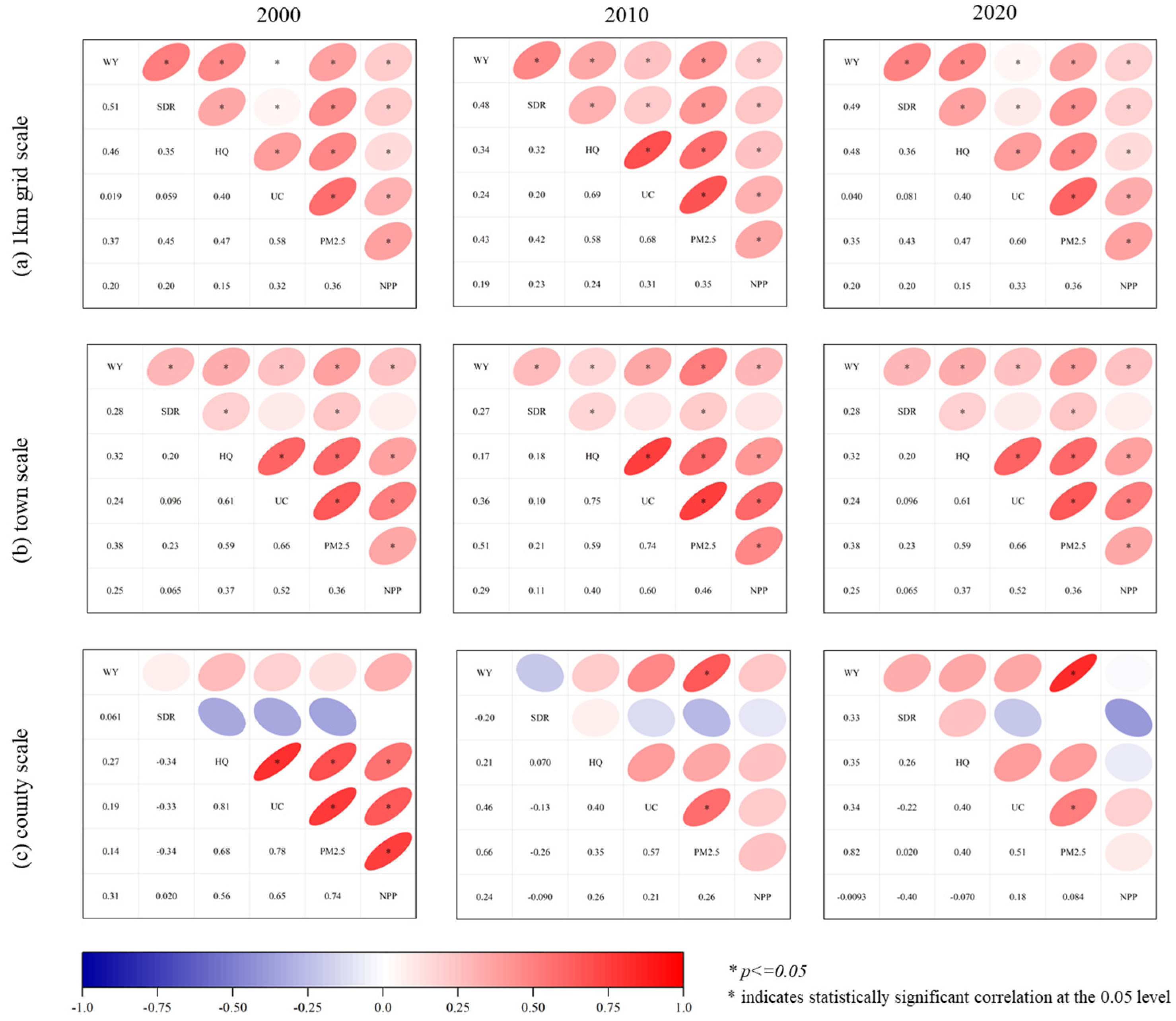
3.2.1. Correlation Analysis of Ess

Multi-scale analysis enhances the accuracy of assessing trade-offs and synergies among ESs. This study examined 15 pairs of potential correlations among six ESs in the years 2000, 2010, and 2020 at three spatial scales: 1 km² grid, township, and county levels (Figure 5). The results indicate that at the county scale, the ESDRs of water yield (WY) and soil retention (SDR) exhibited a positive synergy in 2000 and 2010 (correlation coefficients of 0.51 and 0.28, respectively), but shifted to a weak trade-off at the 1 km grid scale in 2020 (correlation coefficient of −0.20). The ESDRs of habitat quality (HQ) and net primary productivity (NPP) showed strong positive correlations across all scales and years, with coefficients ranging from 0.80 to 0.84. In contrast, the relationship between urban cooling (UC) and PM_2.5 removal services exhibited scale dependency—positively correlated at the county scale (e.g., 0.66 in 2010), but shifted to a trade-off at the 1 km grid scale in 2020 (correlation coefficient of −0.26). From 2000 to 2020, the trade-off between UC and HQ intensified, with the correlation coefficient decreasing from 0.24 to −0.13. Specifically, the relationships between the ESDRs of WY and SDR or UC, and between PM_2.5 removal and SDR or HQ, showed the most significant changes across scales, highlighting the complexity introduced by spatial heterogeneity and varying management demands.

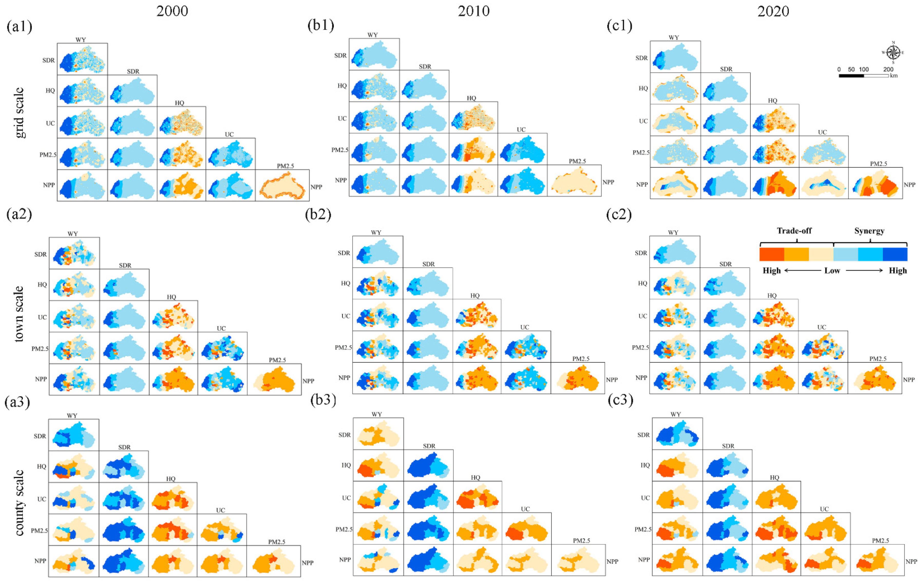
3.2.2. Spatial Patterns of Trade-Offs and Synergies Among Ess

Based on the GWR model results for the years 2000, 2010, and 2020 (Figure 6), ES pairs in Xingtai City demonstrated significant spatial heterogeneity and temporal evolution in their trade-off and synergy relationships across the 1 km grid, township, and county scales. Pairs such as WY-SDR, WY-NPP, and SDR-HQ consistently exhibited strong spatial synergies, mainly concentrated in the western hilly regions and central areas with high ecological functions. These synergies intensified over time, with their spatial distribution shifting from dispersed to more aggregated patterns. In contrast, service pairs such as UC-PM_2.5, PM_2.5-NPP, and HQ-UC generally showed trade-off relationships across all three scales. The trade-off areas were primarily located in the eastern built-up zones and their expansion belts, and their spatial extent gradually increased from 2000 to 2020. Certain pairs like WY-HQ and SDR-NPP exhibited weak synergies at finer scales but tended to stabilize at the county level, suggesting that scaling up helps smooth local variability and highlight dominant relationships. Regulatory service pairs such as HQ-NPP and UC-NPP showed moderate synergies at the grid scale, which weakened or even reversed into trade-offs as the scale increased. Overall, synergies between provisioning and regulating services exhibited a notable strengthening trend, while trade-offs between regulating and environmentally adverse services expanded spatially alongside urbanization, reflecting typical scale-dependent responses and regional differentiation.

3.3. Analysis of Driving Factors

3.3.1. Interpretability Analysis Based on XGBoost Regression and SHAP Models

As shown in Figure 7, the model demonstrates the operational parameters of six types of ESs, all of which exhibit strong predictive performance and generalization ability in Xingtai City. Statistically, the residuals of the six ESs meet the assumptions of the model, indicating good applicability to the data.

Using the XGBoost model combined with SHAP values, this study interprets the ESDR models of six types of ESs, identifies key influencing factors for each service type, and ranks their feature contributions. Overall, the dominant drivers of different ESs vary significantly. For water yield (WY), population density (Pop) shows the highest contribution, followed by elevation (DEM), precipitation (Pre), and cropland proportion (Crop), suggesting that water yield is mainly influenced by topography, hydrology, and population concentration. For soil retention (SDR), DEM, Pre, Crop, and Pop are the main drivers in descending order, indicating that natural topography and agricultural intensity are the key determinants of this service’s supply-demand pattern. For habitat quality (HQ), DEM, urban land proportion (Urban), Crop, and Pop are dominant, reflecting the decisive roles of human development and terrain in shaping habitat service relationships. For urban cooling (UC), Crop, NDVI, temperature (Tem), and Urban are the main contributors, suggesting that vegetation cover and land use structure are vital for regulating this service. NPP is mainly driven by nighttime light intensity (NL), human footprint (HF), NDVI, and Tem, highlighting the combined influence of human disturbance and vegetation activity. For PM_2.5 removal, Tem, NDVI, GDP, and NL are the key drivers, reflecting dependence on both meteorological conditions and urbanization. In summary, although dominant drivers differ across ESs, DEM, NDVI, Pop, and Urban consistently contribute significantly to multiple services, indicating the widespread impact of ecological foundations and human activities on ES supply-demand patterns.

3.3.2. Analysis of Interactive Effects Among Driving Factors

According to the results of interaction analysis in Figure 8, the ESDRs of different ESs exhibit significant responses to interactions among major driving factors, with complex nonlinear characteristics. Among these factor combinations, the interactions between natural and anthropogenic drivers have the most substantial impact on ESDRs, and these effects are highly context-dependent and spatially heterogeneous.

For example, in water yield (WY), there is a pronounced positive interaction between precipitation (Pre) and elevation (DEM). In regions with both high elevation and moderate to high rainfall, the ESDR tends to improve. Conversely, in low-elevation areas, even abundant precipitation cannot significantly enhance WY, indicating the topographic dependency of water retention. For soil retention (SDR), the interaction between Pre and cropland proportion (Crop) is especially notable. In regions with a high proportion of cropland, increased precipitation may exacerbate soil erosion, leading to a decline in SDR, revealing the critical constraint of land-use practices on the regulating capacity of natural factors. For habitat quality (HQ) and urban cooling (UC), the interaction between vegetation cover (NDVI) and urban or population density (Pop) emerges as the dominant factor. Higher NDVI can partially mitigate the negative impacts of intensive construction or dense populations, but its regulatory capacity has limits—when Urban exceeds a threshold (around 20%), the marginal benefit of NDVI declines. Additionally, in UC, NDVI and temperature (Tem) exhibit strong interaction: under high-temperature conditions, NDVI’s contribution to mitigating the urban cooling effect increases significantly, highlighting vegetation’s key role in temperature regulation. Both NPP and PM_2.5 removal services show high sensitivity to anthropogenic drivers. In particular, when GDP, nighttime lights (NLs), and human footprint (HF) interact with natural variables such as NDVI or Tem, the ESDRs of these services display inflection points. For instance, with moderate to high NDVI and low NL, NPP tends to reach optimal levels; however, as NL continues to increase, the ESDR of NPP declines, even when NDVI remains high, reflecting the suppressive impact of urban expansion on the carbon sequestration capacity of ecosystems.

3.3.3. Threshold Effects of Driving Factors

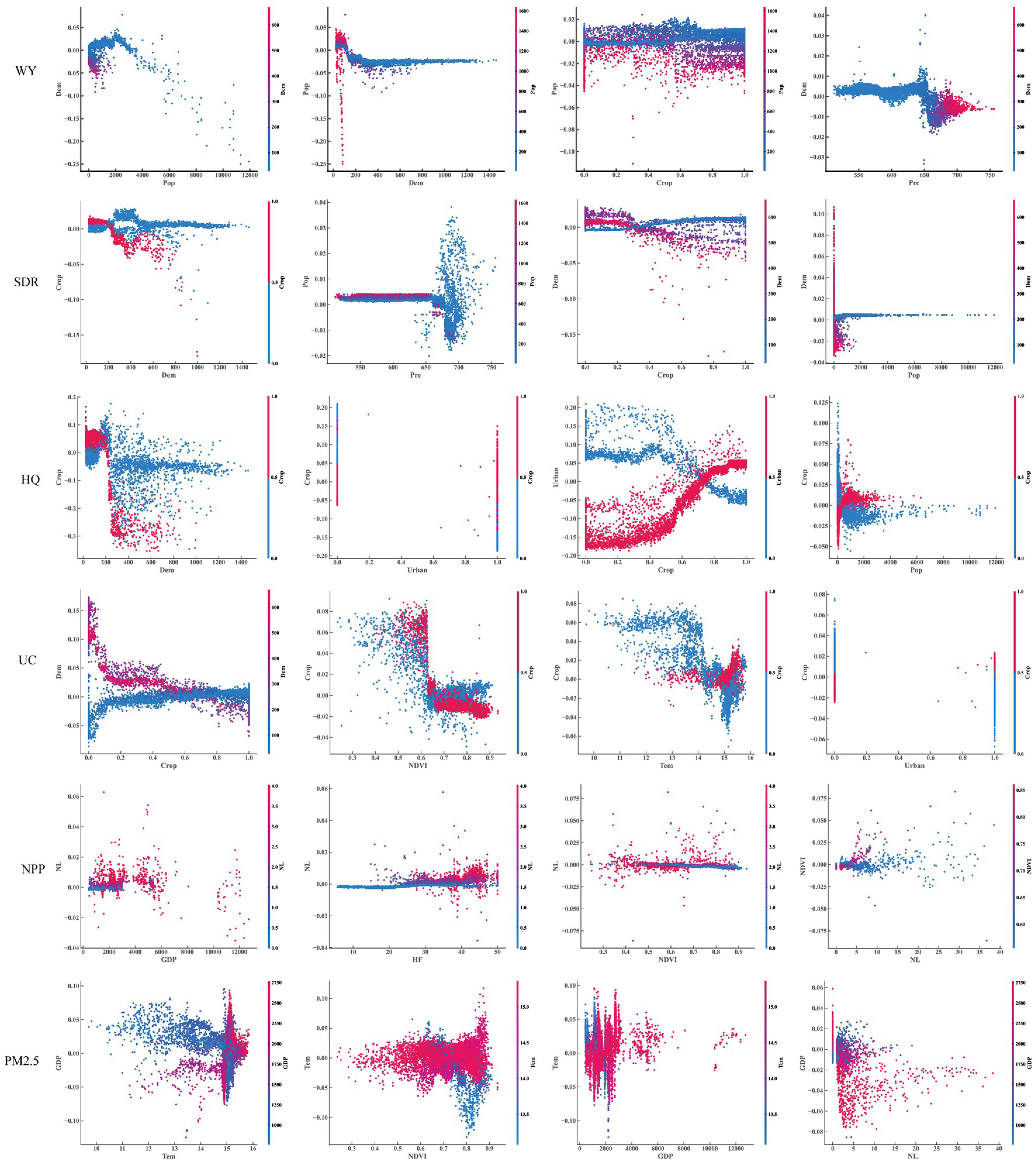
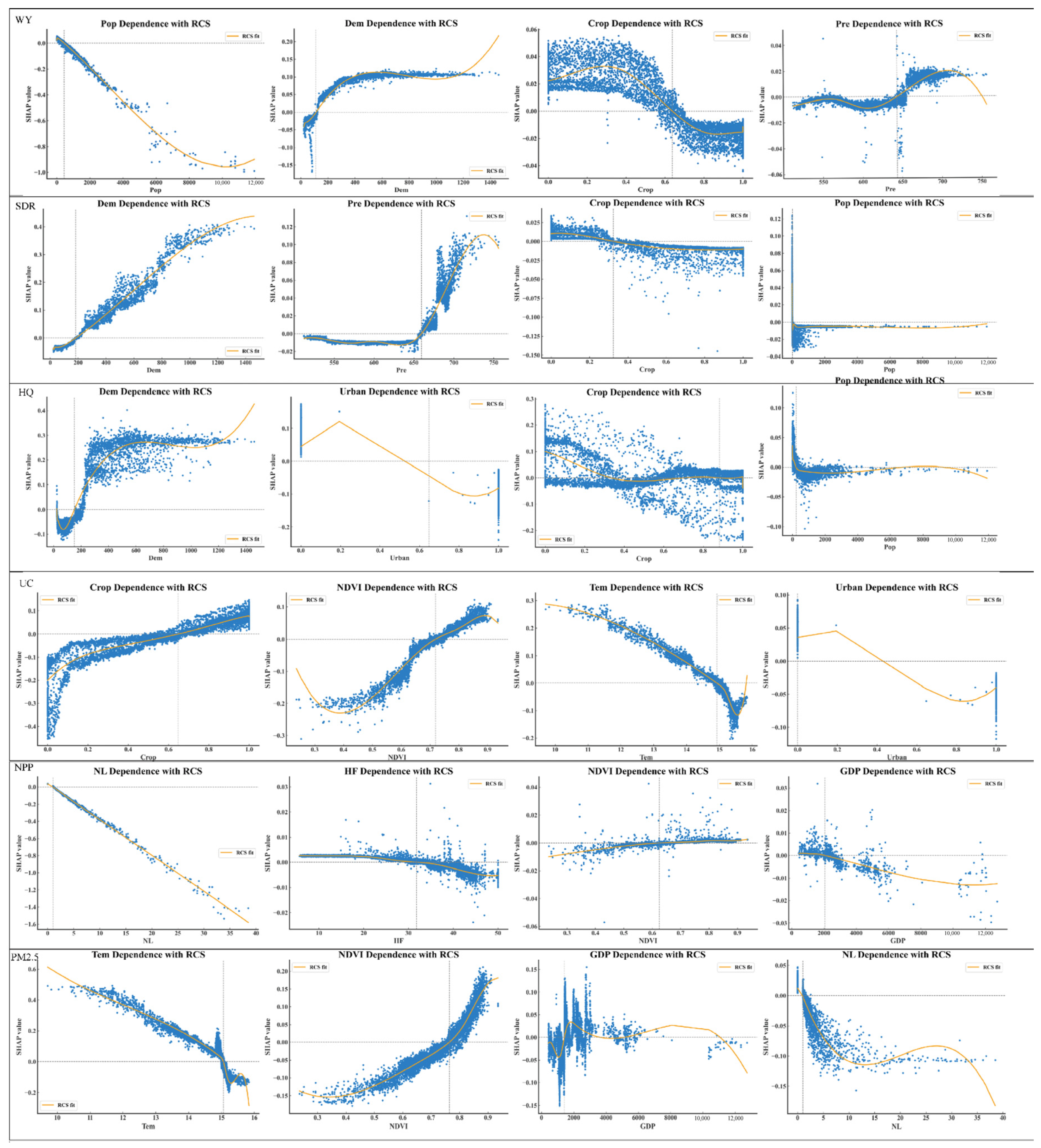
To further explore the nonlinear characteristics and threshold intervals of major driving factors influencing the ESDR, SHAP dependence plots derived from the XGBoost model were fitted using restricted cubic splines (RCS) (Figure 9). This allowed for modeling the marginal response trends and identifying threshold positions of drivers under multivariate interaction contexts. The results indicate that responses of ES ESDRs to most drivers exhibit nonlinear patterns with distinct threshold effects. Population density, urban land proportion, and cropland proportion act as negative drivers for most ESs, and their impacts intensify sharply once critical thresholds are crossed—for example, when population density exceeds 500 people/km² or urban land exceeds 15%, the supply-demand balance deteriorates significantly, reflecting the suppressive effect of anthropogenic pressures on ES provision. In contrast, elevation, NDVI, and precipitation generally act as positive regulators, though their effects plateau or reverse after reaching moderate levels, indicating the presence of marginal effects in natural regulation capacity. Overall, the response of ESs to driving factors is shaped by complex mechanisms involving multivariate interactions, emphasizing the need for supply-demand regulation strategies that account for critical thresholds of human activity and nonlinear modulation by natural factors through differentiated, region-specific approaches.

4. Discussion

4.1. Analysis of ES Supply–Demand Relationships

This study reveals a significant spatial mismatch between ES supply and demand across Xingtai City. High-supply zones are primarily located in the western Taihang mountainous region and designated ecological protection areas, while high-demand zones are concentrated in the densely populated and urbanized eastern and central plains. This spatial divergence pattern aligns with the findings in the coal mining bases of northern Shanxi Province and echoes those in the middle reaches of the Yangtze River Urban Agglomeration, both of which highlight the spatial segregation between “ecological supply zones” and “human demand zones” in resource-based regions [48,49]. Similarly, in southwestern China, this study also identifies the urban-rural fringe as the area with the most pronounced supply–demand mismatch, reflecting the “edge pressure effect” of human activity on ecosystems [50].

In terms of individual ESs, the spatial mismatches are particularly evident for water yield and carbon sequestration. Similarly to the findings in North China, this study finds that water yield is significantly influenced by elevation, slope, and vegetation cover [51]. However, water demand is concentrated in areas characterized by high population density and a high proportion of built-up land. Regarding carbon storage, forest coverage and terrain ruggedness are dominant determinants of supply capacity, while carbon demand tends to peak in economically active zones, resulting in an inverse supply–demand distribution [19]. From a regional and methodological perspective, the observed mismatch patterns in this study are highly comparable to those identified in Jiangxi Province, and form a stark contrast to the “well-coordinated supply–demand pattern” found in the northern Tianshan Economic Belt [52,53].

While previous studies often relied on supply–demand ratios, indices, or pressure indicators, such metrics are often limited in identifying the precise geographic boundaries of spatial mismatch. By conducting analysis at the grid scale and integrating multi-source spatial data, this study enhances spatial resolution and accuracy. Future research is recommended to incorporate dynamic temporal analysis methods, as well as integrate social survey data and policy response simulations to better forecast and regulate ES supply–demand scenarios [54].

4.2. Multi-Scale Trade-Offs and Synergies Among ESs

The variation in trade-offs and synergies across scales reflects the interplay between landscape heterogeneity and human activities in Xingtai. At the 1-km grid scale, fine-grained land-use diversity and vegetation gradients lead to strong local contrasts: mountainous and ecological buffer areas show WY–SDR and HQ–NPP synergies due to high vegetation cover and favorable topography, whereas urban cores exhibit UC–PM_2.5 trade-offs driven by impervious expansion and industrial emissions [55,56]. At the township scale, aggregation moderates these localized effects, producing smoother patterns where ecological processes and socioeconomic factors jointly shape ES coupling. At the county scale, regional planning and land-use policies further weaken fine-scale conflicts, indicating that scale averaging reduces spatial heterogeneity. These multi-scale differences highlight that ES relationships are context-dependent and should be managed with scale-specific ecological and policy strategies [57,58].

With increasing spatial scale, the overall patterns of ES interactions exhibited a smoothing effect. Synergies such as SDR–NPP and HQ–NPP became more pronounced at the township and county levels, revealing larger-scale functional linkages in regional ecosystems [59]. However, finer-scale synergies such as UC–PM_2.5 and HQ–UC diminished or reversed at coarser scales, indicating that spatial heterogeneity and human activity have stronger localized effects [60,61]. Temporally, some synergies—such as WY–SDR and SDR–NPP—intensified in areas undergoing ecological restoration, whereas trade-offs, especially HQ–UC and UC–PM_2.5, expanded in peri-urban zones due to continued urban sprawl. These dynamics mirror those reported in studies of other northern Chinese urban agglomerations and confirm the dual influence of ecological engineering and urbanization on service coupling mechanisms [62].

The spatial coupling analysis indicates a clear geographic differentiation: HQ–NPP synergies dominate in western forested and grassland zones, while severe UC–PM_2.5 trade-offs concentrate in eastern industrial belts and urban corridors. These patterns are consistent with local landscape and anthropogenic drivers: high vegetation cover and favorable topography in the west reinforce hydrological and habitat functions, whereas urban expansion, increased imperviousness and industrial emissions in the east degrade habitat integrity while elevating thermal and air-pollution regulation pressures. The observed scale-dependent smoothing—where fine-scale trade-offs (e.g., UC–PM_2.5) weaken at township and county scales—underscores that aggregation can mask localized conflicts; therefore, policy responses should be scale-aware. Temporal trajectories further show that synergies such as WY–SDR have intensified in restoration areas, whereas UC–PM_2.5 trade-offs have expanded with peri-urbanization. Together, these results highlight the need for area-targeted management that aligns restoration priorities with local drivers (e.g., reforestation in ecological buffers. emission controls, and low-impact urban design in industrial corridors). We note, however, that while our multi-method approach reduces the risk of misattributing causality, formal causal testing remains a priority for follow-up research [63,64].

4.3. Analysis of Driving Factors of ESs

Using an XGBoost–SHAP framework, this study systematically identified the key drivers influencing the supply–demand ratios of six ES categories in Xingtai City. Among these, variables such as elevation (DEM), vegetation index (NDVI), cropland proportion (Crop), and population density (Pop) consistently emerged as dominant across multiple services, indicating their stable and recurrent influence. These findings are consistent with previous studies, which emphasize the leading role of natural factors in regulating services [15,65]. They also corroborate the trend observed, whereby intensified human activities exacerbate mismatches between ES supply and demand, particularly in East China [66]. Specifically, water yield and soil retention services were mainly driven by precipitation, terrain, and land-use composition, echoing the conclusions of in the Loess Plateau [67]. In contrast, urban cooling and PM_2.5 removal services showed heightened sensitivity to anthropogenic indicators such as population density, nighttime light intensity, and built-up land area. These patterns align with findings from the Beijing–Tianjin–Hebei region and the Southwest Karst–Beibu Gulf zone [68,69].

Notably, the importance of individual drivers varied considerably across service types. For instance, NDVI and temperature were the primary factors influencing net primary productivity (NPP), highlighting its function as a proxy for the ecosystem’s baseline productivity. This finding is consistent with previous multi-scale ES modeling results [52,70]. In contrast, built-up land and GDP consistently exhibited negative associations with multiple ESs, underscoring the suppressive effects of rapid urbanization on ecological functions, which aligns with earlier studies on urban expansion and ecological degradation [39,71].

At the regional level, the driving mechanisms of ES supply–demand relationships in Xingtai exhibit both general features of resource-based cities characterized by high-intensity land development, and the distinctive compound influences of its mountain–plain–urban geomorphological mosaic. These insights reinforce the multi-factor spatial differentiation mechanisms reported in northern Chinese city clusters and broaden the conceptual framework regarding ES heterogeneity and driver coupling relationships [45,72]. While elevation, NDVI, cropland proportion and population density emerge as consistent drivers at the regional scale, we emphasize that these variables provide a high-level synthesis rather than a complete description of all local mechanisms. The use of XGBoost–SHAP and spatially explicit GWR analyses helps to reveal nonlinearities and geographic heterogeneity; however, transition zones and industrial legacy areas (e.g., coal mining belts) may involve additional processes—such as soil contamination, mine subsidence, and post-mining land-use succession—not captured by our current predictors. We therefore recommend targeted stratified analyses and the incorporation of mining activity indices, soil pollution data, and reclamation history in future work to better explain ES dynamics in these special landscapes. In conclusion, the identification of service-specific key drivers has strategic implications for promoting synergy between ecological conservation and high-quality development.

4.4. Limitations and Future Directions

This study identifies the trade-offs and synergies among ecosystem services in Xingtai through a multi-scale analysis and further examines their driving mechanisms using the XGBoost–SHAP model, with the aim of clarifying the interaction characteristics of ecosystem services and their influencing factors across different spatial levels. While the methodological innovation lies in integrating XGBoost’s nonlinear modeling strength with SHAP’s interpretability to achieve prioritized identification of driver importance, thereby overcoming limitations of traditional statistical methods in variable effect detection, three main limitations persist: First, following the United Nations Millennium Ecosystem Assessment (MA) classification of ESs into four classes (provisioning, regulating, supporting, and cultural) and subtypes, this study only evaluated six ESs (water yield, soil retention, habitat quality, urban cooling, NPP, and PM_2.5 removal), which may not fully represent all ES types in Xingtai, necessitating future assessments of additional Ess; Second, while Spearman correlation analysis was applied to explore linear relationships between ES pairs, its inability to account for nonlinear interactions or confounding variables—despite supplementary curve estimation—highlights the need for advanced methods like structural equation modeling (SEM) or network analysis to infer causality in future work; Third, Although SHAP analysis quantifies the relative importance and nonlinear interactions of multiple drivers, it primarily reflects statistical associations rather than explicit ecological processes. Future research should therefore integrate SHAP-based insights with process-based ecological models—such as hydrological, nutrient cycling, and landscape evolution simulations—to better interpret the biophysical mechanisms underlying the observed effects. Incorporating long-term monitoring data, field experiments, and causal inference frameworks will further enhance our understanding of how human and natural drivers jointly shape ES dynamics [73].

5. Conclusions

From 2000 to 2020, the average ESDRs of six ESs in Xingtai City exhibited temporal fluctuations. Among these, five ESs (excluding soil retention (SR), habitat quality (HQ), and water yield (WY)) demonstrated overall increasing trends over the past 12 years. Spatial heterogeneity was significant across all ESs, with high-value ecological supply zones predominantly located in the western mountainous regions, while the eastern plains showed relatively lower values, forming a distinct “west-high-east-low” gradient pattern. Pairwise ES relationships in Xingtai City were primarily synergistic, with most correlation coefficients showing an “initial weakening followed by subsequent strengthening” trend over time. Notably, synergistic relationships between regulating and supporting services exhibited temporal stability across spatial scales, though their intensity tended to increase with spatial scale expansion. In contrast, interactions between provisioning services and other ESs displayed marked spatial scale variability and temporal fluctuations. At the 1-km grid scale, elevation (Dem), normalized difference vegetation index (NDVI), cropland proportion (Crop), and population density (Pop) emerged as recurrent drivers influencing ESDRs of all six ESs. These variables collectively dominated the spatial differentiation of ESs, underscoring their critical roles in shaping ecological service patterns in the study area. Beyond empirical findings, this study also highlights the methodological advantages of the XGBoost–SHAP framework as a novel approach for exploring ES dynamics. By combining the predictive capability of machine learning with the interpretability of SHAP analysis, this framework effectively uncovers nonlinear and scale-dependent relationships between ecological drivers and service outcomes. This methodological framework is not limited to Xingtai City but can be flexibly applied to other regions to support integrated land-use management, ecological restoration planning, and sustainability assessments.

References

1. Costanza, R. Valuing Natural Capital and Ecosystem Services toward the Goals of Efficiency, Fairness, and Sustainability. Ecosyst. Serv. 2020, 43, 101096. [Google Scholar] [CrossRef]
2. Daily, G.C. Nature’s Services: Societal Dependence on Natural Ecosystems; Island Pr: Miami, FL, USA, 1997; ISBN 1-55963-476-6. [Google Scholar]
3. Gao, J.; Zuo, L. Revealing Ecosystem Services Relationships and Their Driving Factors for Five Basins of Beijing. J. Geogr. Sci. 2021, 31, 111–129. [Google Scholar] [CrossRef]
4. Li, P.; Li, T. Spatiotemporal Analysis of Ecosystem Services and the Impact of New-Type Urbanization: A Case Study of Chengdu, China. Ecol. Indic. 2025, 171, 113191. [Google Scholar] [CrossRef]
5. Reid, W.V.; Mooney, H.A.; Cropper, A.; Capistrano, D.; Carpenter, S.R.; Chopra, K.; Dasgupta, P.; Dietz, T.; Duraiappah, A.K.; Hassan, R. Ecosystems and Human Well-Being-Synthesis: A Report of the Millennium Ecosystem Assessment; Island Press: Washington, DC, USA, 2005; ISBN 1-59726-040-1. [Google Scholar]
6. Fulford, R.S.; Russell, M.; Myers, M.; Malish, M.; Delmaine, A. Models Help Set Ecosystem Service Baselines for Restoration Assessment. J. Environ. Manag. 2022, 317, 115411. [Google Scholar] [CrossRef]
7. Costanza, R.; d’Arge, R.; De Groot, R.; Farber, S.; Grasso, M.; Hannon, B.; Limburg, K.; Naeem, S.; O’neill, R.V.; Paruelo, J. The Value of the World’s Ecosystem Services and Natural Capital. Nature 1997, 387, 253–260. [Google Scholar] [CrossRef]
8. Burkhard, B.; Kroll, F.; Nedkov, S.; Müller, F. Mapping Ecosystem Service Supply, Demand and Budgets. Ecol. Indic. 2012, 21, 17–29. [Google Scholar] [CrossRef]
9. Dang, H.; Li, J.; Zhou, Z. Revealing the Supply-Demand Relationship of Urban Cultural Ecosystem Services: The Combination of Open-Source Spatial Model and Topic Model. Appl. Geogr. 2024, 167, 103288. [Google Scholar] [CrossRef]
10. Tallis, H.; Kareiva, P.; Marvier, M.; Chang, A. An Ecosystem Services Framework to Support Both Practical Conservation and Economic Development. Proc. Natl. Acad. Sci. USA 2008, 105, 9457–9464. [Google Scholar] [CrossRef]
11. Cord, A.F.; Bartkowski, B.; Beckmann, M.; Dittrich, A.; Hermans-Neumann, K.; Kaim, A.; Lienhoop, N.; Locher-Krause, K.; Priess, J.; Schröter-Schlaack, C.; et al. Towards Systematic Analyses of Ecosystem Service Trade-Offs and Synergies: Main Concepts, Methods and the Road Ahead. Ecosyst. Serv. 2017, 28, 264–272. [Google Scholar] [CrossRef]
12. Stoeckl, N.; Costanza, R.; Dorji, N.; Kubiszewski, I.; Limenih, B.; Tian, J.; Yamazaki, S. Valuing the Reciprocating Services That Humans Can Provide to Ecosystems. Ecol. Indic. 2025, 174, 113496. [Google Scholar] [CrossRef]
13. Luo, H.; Zhang, Z.; Zhu, Q.; Houda Ben Ameur, N.E.; Liu, X.; Ding, F.; Cai, Y. Using Large Language Models to Investigate Cultural Ecosystem Services Perceptions: A Few-Shot and Prompt Method. Landsc. Urban Plan. 2025, 258, 105323. [Google Scholar] [CrossRef]
14. Gao, Y.; Fu, D.; Huang, H.; Jiang, J.; Liu, Q.; Zhu, L.; Ding, G. Spatio-Temporal Evolution and Scenario-Based Optimization of Urban Ecosystem Services Supply and Demand: A Block-Scale Study in Xiamen, China. Ecol. Indic. 2025, 172, 113289. [Google Scholar] [CrossRef]
15. Chang, B.; Chen, B.; Chen, W.; Xu, S.; He, X.; Yao, J.; Huang, Y. Analysis of Trade-off and Synergy of Ecosystem Services and Driving Forces in Urban Agglomerations in Northern China. Ecol. Indic. 2024, 165, 112210. [Google Scholar] [CrossRef]
16. Luan, C.; Liu, R.; Li, Y.; Zhang, Q. Comparison of Various Models for Multi-Scenario Simulation of Land Use/Land Cover to Predict Ecosystem Service Value: A Case Study of Harbin-Changchun Urban Agglomeration, China. J. Clean. Prod. 2024, 478, 144012. [Google Scholar] [CrossRef]
17. Wu, Q.; Cao, Y.; Su, D.; Cao, Y. A Multi-Scale Framework for Understanding Spatial Scale Effects on Ecosystem Service Heterogeneity, Interactions, Drivers and Their Socio-Ecological Impact Pathways for Adaptive Management. J. Clean. Prod. 2025, 516, 145757. [Google Scholar] [CrossRef]
18. Uribe-Aguado, J.; Patiño, J.N.; Kozak, D.; Wild, T.; Sánchez, J.P.R. A Decision Support Tool for the Selection of Biophysical Methodologies to Assess Urban Nature-Based Solutions Using Regulating Ecosystem Services. Urban For. Urban Green. 2025, 128842. [Google Scholar] [CrossRef]
19. Gao, M.; Hu, Y.; Liu, X.; Liang, M. Revealing Multi-Scale Characteristics of Ecosystem Services Supply and Demand Imbalance to Enhance Refined Ecosystem Management in China. Ecol. Indic. 2025, 170, 112971. [Google Scholar] [CrossRef]
20. Rong, Y.; Li, K.; Guo, J.; Zheng, L.; Luo, Y.; Yan, Y.; Wang, C.; Zhao, C.; Shang, X.; Wang, Z. Multi-Scale Spatio-Temporal Analysis of Soil Conservation Service Based on MGWR Model: A Case of Beijing-Tianjin-Hebei, China. Ecol. Indic. 2022, 139, 108946. [Google Scholar] [CrossRef]
21. Dang, L.; Zhao, F.; Teng, Y.; Teng, J.; Zhan, J.; Zhang, F.; Liu, W.; Wang, L. Scale Dependency of Trade-Offs/Synergies Analysis of Ecosystem Services Based on Bayesian Belief Networks: A Case of the Yellow River Basin. J. Environ. Manage. 2025, 375, 124410. [Google Scholar] [CrossRef]
22. Zhang, J.; Zhang, Z.; Liu, L.; Cao, Y.; Zhang, M.; Yuan, Z.; Ma, R.; Liu, X.; Liu, Y. Scaling Effects of Ecosystem Service Trade-off and Synergy in Arid Inland River Basins: A Case Study of the Manas River Basin of Xinjiang, China. Ecol. Indic. 2025, 173, 113358. [Google Scholar] [CrossRef]
23. Lyu, F.; Tang, J.; Olhnuud, A.; Hao, F.; Gong, C. The Impact of Large-Scale Ecological Restoration Projects on Trade-Offs/Synergies and Clusters of Ecosystem Services. J. Environ. Manag. 2024, 365, 121591. [Google Scholar] [CrossRef]
24. Qiao, X.; Gu, Y.; Zou, C.; Xu, D.; Wang, L.; Ye, X.; Yang, Y.; Huang, X. Temporal Variation and Spatial Scale Dependency of the Trade-Offs and Synergies among Multiple Ecosystem Services in the Taihu Lake Basin of China. Sci. Total Environ. 2019, 651, 218–229. [Google Scholar] [CrossRef]
25. Li, T.; Li, D.; Liu, Y.; Wei, G.; Liu, C.; Wang, J. The Spatiotemporal Effects on Ecosystem Services Supply-Demand from Industrial Transformation and Upgrading: Promotion or Inhibition? Ecol. Indic. 2024, 161, 111990. [Google Scholar] [CrossRef]
26. Zhang, H.; Wang, L.; Jiang, S.; Li, K.; Xin, X.; Huang, X.; Chen, J.; Zhou, L.; Li, Z. Impacts of Rice–Crayfish Co-Culture on Ecosystem Service Trade-Offs/Synergies in Agricultural Watersheds: A Case Exploration in Sihu Lake Basin, China. Agric. Water Manag. 2025, 310, 109389. [Google Scholar] [CrossRef]
27. Salata, S.; Grillenzoni, C. A Spatial Evaluation of Multifunctional Ecosystem Service Networks Using Principal Component Analysis: A Case of Study in Turin, Italy. Ecol. Indic. 2021, 127, 107758. [Google Scholar] [CrossRef]
28. Tonin, S. Influence of Environmental Attitudes and Time Horizons on the Valuation of Lagoon Ecosystem Services: A Choice Experiment Approach Using Principal Component Analysis. J. Environ. Manag. 2025, 375, 124178. [Google Scholar] [CrossRef]
29. Zhou, J.; Yang, J.; Tang, Z.; Xue, L.; Zhang, W.; Zhang, J. Driving Mechanisms of Ecosystem Services and Their Trade-Offs and Synergies in the Transition Zone between the Qinghai-Tibet Plateau and the Loess Plateau. Ecol. Indic. 2025, 171, 113148. [Google Scholar] [CrossRef]
30. Zhao, T.; Pan, J. Ecosystem Service Trade-Offs and Spatial Non-Stationary Responses to Influencing Factors in the Loess Hilly-Gully Region: Lanzhou City, China. Sci. Total Environ. 2022, 846, 157422. [Google Scholar] [CrossRef] [PubMed]
31. Gu, Y.; Chen, Y.; Yang, D.; Zhao, X.; Pan, S. The Impact of Impervious Surface Expansion Morphology on Ecosystem Services and Thresholds in the Haihe River Basin. Ecol. Indic. 2025, 175, 113493. [Google Scholar] [CrossRef]
32. Liu, T.; Wang, M.; Wang, M.; Xiong, Q.; Jia, L.; Ma, W.; Sui, S.; Wu, W.; Guo, X. Identification of the Primary Pollution Sources and Dominant Influencing Factors of Soil Heavy Metals Using a Random Forest Model Optimized by Genetic Algorithm Coupled with Geodetector. Ecotoxicol. Environ. Saf. 2025, 290, 117731. [Google Scholar] [CrossRef]
33. Yang, L.; Liu, Y.; Liu, Y.; Liu, R. Spatial-Temporal Dynamics and Drivers of Ecosystem Service Interactions along the Yellow River Area in Shaanxi Province. J. Clean. Prod. 2025, 496, 145095. [Google Scholar] [CrossRef]
34. Rodrigues, M.; Jiménez-Ruano, A.; Peña-Angulo, D.; de la Riva, J. A Comprehensive Spatial-Temporal Analysis of Driving Factors of Human-Caused Wildfires in Spain Using Geographically Weighted Logistic Regression. J. Environ. Manag. 2018, 225, 177–192. [Google Scholar] [CrossRef] [PubMed]
35. Huang, X.; Wang, Y.; Wang, X.; Chen, J.; Ma, J.; Liang, E.; Wang, X. Exploring the Natural-Socioeconomic Driving and Response Mechanisms of Ecosystem Services Interactions to Optimize Ecosystem Management: A Case Study in the Yarlung Zangbo River Basin. Sci. Total Environ. 2024, 957, 177842. [Google Scholar] [CrossRef] [PubMed]
36. Bacani, V.M.; Machado da Silva, B.H.; Ayumi de Souza Amede Sato, A.; Souza Sampaio, B.D.; Rodrigues da Cunha, E.; Pereira Vick, E.; Ribeiro de Oliveira, V.F.; Decco, H.F. Carbon Storage and Sequestration in a Eucalyptus Productive Zone in the Brazilian Cerrado, Using the ca-Markov/Random Forest and InVEST Models. J. Clean. Prod. 2024, 444, 141291. [Google Scholar] [CrossRef]
37. Li, T.; Wu, Y.; Ren, F.; Li, M. Estimation of Unrealized Forest Carbon Potential in China Using Time-Varying Boruta-SHAP-Random Forest Model and Climate Vegetation Productivity Index. J. Environ. Manag. 2025, 377, 124649. [Google Scholar] [CrossRef]
38. Yang, M.; Chen, Y.; Yang, Y.; Yan, Y. Nonlinear Relationship and Threshold-Based Zones between Ecosystem Service Supply-Demand Ratio and Land Use Intensity: A Case Study of the Beijing-Tianjin-Hebei Region, China. J. Clean. Prod. 2024, 481, 144148. [Google Scholar] [CrossRef]
39. Qu, J.; Xu, Z.; Dong, B.; Wang, H.; Han, Y. Analyzing Trade-Offs, Synergies, and Driving Factors of Ecosystem Services in Anhui Province Using Spatial Analysis and XG-Boost Modeling. Ecol. Indic. 2025, 171, 113098. [Google Scholar] [CrossRef]
40. Sokhansefat, S.; Kanani-Sadat, Y.; Nasseri, M. Modeling Vegetation Dynamics in Complex Topography under Impacts of Climate Change: Integration of Spatial Clustering and Optimized XGBoost. J. Environ. Manag. 2025, 387, 125902. [Google Scholar] [CrossRef]
41. Tian, Y.; Zhang, Q.; Tao, J.; Zhang, Y.; Lin, J.; Bai, X. Use of Interpretable Machine Learning for Understanding Ecosystem Service Trade-Offs and Their Driving Mechanisms in Karst Peak-Cluster Depression Basin, China. Ecol. Indic. 2024, 166, 112474. [Google Scholar] [CrossRef]
42. Wang, H.; Yuan, W.; Ma, Y.; Bai, X.; Huang, L.; Cheng, S.; Yang, H.; Guo, W. Spatiotemporal Dislocation of Ecosystem Supply and Demand Services from Habitat Quality under Different Development Scenarios. Ecol. Indic. 2023, 157, 111230. [Google Scholar] [CrossRef]
43. Chen, T.; Feng, Z.; Zhao, H.; Wu, K. Identification of Ecosystem Service Bundles and Driving Factors in Beijing and Its Surrounding Areas. Sci. Total Environ. 2020, 711, 134687. [Google Scholar] [CrossRef]
44. Sharp, R.; Douglass, J.; Wolny, S.; Arkema, K.; Bernhardt, J.; Bierbower, W. InVEST 3.6. 0 User’s Guide. Collaborative Publication by the Natural Capital Project, Stanford University, the University of Minnesota, the Nature Conservancy, and the World Wildlife Fund. In The Nature Conservancy, and the World Wildlife Fund; Stanford University: Stanford, CA, USA, 2018. [Google Scholar]
45. Yang, Y.; Yuan, X.; An, J.; Su, Q.; Chen, B. Drivers of Ecosystem Services and Their Trade-Offs and Synergies in Different Land Use Policy Zones of Shaanxi Province, China. J. Clean. Prod. 2024, 452, 142077. [Google Scholar] [CrossRef]
46. Xu, Y.; Li, C. Investigating the Heterogeneity of Driving Mechanisms and Multi-Dimensional Policy Pathways in Ecosystem Service Supply-Demand Relationships: A Case Study of the Shandong Peninsula Urban Agglomeration. J. Clean. Prod. 2025, 512, 145523. [Google Scholar] [CrossRef]
47. Fan, J.; Liu, S.; Wang, W.; Li, Y.; Wang, Z.; Liu, M.; Zhao, Y.; Lin, J.; Tian, Z.; Wu, G. Identifying Driving Mechanisms and Relationships between Supply and Demand of Ecosystem Services Based on Structural Equation Model in the Upstream Segment of the Yangtze River. J. Environ. Manag. 2025, 393, 127093. [Google Scholar] [CrossRef] [PubMed]
48. Jia, Q.; Jiao, L.; Lian, X.; Wang, W. Linking Supply-Demand Balance of Ecosystem Services to Identify Ecological Security Patterns in Urban Agglomerations. Sustain. Cities Soc. 2023, 92, 104497. [Google Scholar] [CrossRef]
49. Jing, Z.; Min, X.; Li, S.; Li, J.; Song, W. Trade-off or Synergy? The Impacts of Coal Energy Consumption on Compound System Vulnerability: A Perspective from Coal Resource Base Assessment. Ecol. Indic. 2025, 170, 113124. [Google Scholar] [CrossRef]
50. Li, W.; Kang, J.; Wang, Y. Integrating Ecosystem Services Supply-Demand Balance into Landscape Ecological Risk and Its Driving Forces Assessment in Southwest China. J. Clean. Prod. 2024, 475, 143671. [Google Scholar] [CrossRef]
51. Ding, H.; Sun, R. Supply-Demand Analysis of Ecosystem Services Based on Socioeconomic and Climate Scenarios in North China. Ecol. Indic. 2023, 146, 109906. [Google Scholar] [CrossRef]
52. Tian, F.; Li, X.; Wu, X.; Gong, L. Identifying Supply–Demand Mismatches of Ecosystem Services and Social-Ecological Drivers at Different Scales to Support Land Use Planning. Ecol. Indic. 2025, 174, 113462. [Google Scholar] [CrossRef]
53. Su, B.; Liu, M. Coupling Management Ecosystem Service Supply-Supply Trade-Offs and Supply–Demand Trade-Offs: Framework and Practice. Ecol. Indic. 2024, 166, 112258. [Google Scholar] [CrossRef]
54. Shen, J.; Li, S.; Wang, H.; Wu, S.; Liang, Z.; Zhang, Y.; Wei, F.; Li, S.; Ma, L.; Wang, Y.; et al. Understanding the Spatial Relationships and Drivers of Ecosystem Service Supply-Demand Mismatches towards Spatially-Targeted Management of Social-Ecological System. J. Clean. Prod. 2023, 406, 136882. [Google Scholar] [CrossRef]
55. Liu, J.; Pei, X.; Zhu, W.; Jiao, J. Understanding the Intricate Tradeoffs among Ecosystem Services in the Beijing-Tianjin-Hebei Urban Agglomeration across Spatiotemporal Features. Sci. Total Environ. 2023, 898, 165453. [Google Scholar] [CrossRef]
56. Guo, X.; Fang, C.; Mu, X.; Chen, D. Coupling and Coordination Analysis of Urbanization and Ecosystem Service Value in Beijing-Tianjin-Hebei Urban Agglomeration. Ecol. Indic. 2022, 137, 108782. [Google Scholar] [CrossRef]
57. Zhai, Y.; Zhai, G.; Yu, Z.; Lu, Z.; Chen, Y.; Liu, J. Coupling Coordination between Urbanization and Ecosystem Services Value in the Beijing-Tianjin-Hebei Urban Agglomeration. Sustain. Cities Soc. 2024, 113, 105715. [Google Scholar] [CrossRef]
58. Zhang, X.; Du, J.; Huang, T.; Zhang, L.; Gao, H.; Zhao, Y.; Ma, J. Atmospheric Removal of PM 2.5 by Man-Made Three Northern Regions Shelter Forest in Northern China Estimated Using Satellite Retrieved PM 2.5 Concentration. Sci. Total Environ. 2017, 593–594, 713–721. [Google Scholar] [CrossRef] [PubMed]
59. Haase, D.; Schwarz, N.; Strohbach, M.; Kroll, F.; Seppelt, R. Synergies, Trade-Offs, and Losses of Ecosystem Services in Urban Regions: An Integrated Multiscale Framework Applied to the Leipzig-Halle Region, Germany. Ecol. Soc. 2012, 17, 22. [Google Scholar] [CrossRef]
60. Li, S.; Xiang, N.; Shu, C.; Xu, F. Unveiling the Industrial Synergy Optimization Pathways in Beijing-Tianjin-Hebei Urban Agglomeration Based on Water-Energy-Carbon Nexus. J. Environ. Manag. 2025, 376, 124528. [Google Scholar] [CrossRef]
61. Yan, Y.; Yang, Y.; Yang, M. Unravelling the Non-Linear Response of Ecosystem Services to Urban-Rural Transformation in the Beijing-Tianjin-Hebei Region, China. Ecol. Inform. 2024, 81, 102633. [Google Scholar] [CrossRef]
62. Li, Q.; Li, D.; Wang, J.; Wang, S.; Wang, R.; Fu, G.; Yuan, Y.; Zheng, Z. Spatial Heterogeneity of Ecosystem Service Bundles and the Driving Factors in the Beijing-Tianjin-Hebei Region. J. Clean. Prod. 2024, 479, 144006. [Google Scholar] [CrossRef]
63. Deng, F.; Zhu, S.; Guo, J.; Sun, X. Exploring the Quality of Ecosystem Services and the Segmental Impact of Influencing Factors in Resource-Based Cities. J. Environ. Manage. 2025, 375, 124411. [Google Scholar] [CrossRef]
64. Wang, S.; Zhao, Y.; Wang, Q.; Ren, H.; Zhu, S.; Cao, J. Ecological Network Construction and Optimization of Typical Resource-Based Regions, and Strategies for the Enhancement of Multiple Ecosystem Services: Balancing Function and Structure. Ecol. Indic. 2025, 170, 112951. [Google Scholar] [CrossRef]
65. Bi, S.; Li, Z.; Chen, Y.; Zhang, Q.; Ye, T. Identification of Priority Conservation Areas in Beijing-Tianjin-Hebei Using Multi-Scenario Trade-Offs Based on Different Spatial Scales and Their Drivers. Ecol. Indic. 2024, 166, 112508. [Google Scholar] [CrossRef]
66. Zhang, X.; Han, R.; Yang, S.; Yang, Y.; Tang, X.; Qu, W. Identification of Bundles and Driving Factors of Ecosystem Services at Multiple Scales in the Eastern China Region. Ecol. Indic. 2024, 158, 111378. [Google Scholar] [CrossRef]
67. Xu, T.; Tian, G.; Lin, T.; Li, W.; Liu, C. Multiscale Analysis of Ecosystem Service Interactions and Driving Factors in the Loess Plateau: Implications for Ecological Management. J. Clean. Prod. 2025, 495, 145074. [Google Scholar] [CrossRef]
68. Shen, J.; Li, S.; Liu, L.; Liang, Z.; Wang, Y.; Wang, H.; Wu, S. Uncovering the Relationships between Ecosystem Services and Social-Ecological Drivers at Different Spatial Scales in the Beijing-Tianjin-Hebei Region. J. Clean. Prod. 2021, 290, 125193. [Google Scholar] [CrossRef]
69. Gao, C.; Hu, B.; Wang, Z.; Huang, S.; Zhang, L. Study on Spatiotemporal Changes of Ecosystem Service Trade-Offs/Synergies and Driving Mechanisms in the Key Zone of Mountain-River-Sea Coupling: A Case Study of the Southwest Guangxi Karst-Beibu Gulf. Ecol. Indic. 2024, 169, 112892. [Google Scholar] [CrossRef]
70. Liu, Q.; Qiao, J.; Li, M.; Huang, M. Spatiotemporal Heterogeneity of Ecosystem Service Interactions and Their Drivers at Different Spatial Scales in the Yellow River Basin. Sci. Total Environ. 2024, 908, 168486. [Google Scholar] [CrossRef]
71. Lv, L.; Han, X.; Zhu, J.; Liao, K.; Yang, Q.; Wang, X. Spatial Drivers of Ecosystem Services Supply-Demand Balances in the Nanjing Metropolitan Area, China. J. Clean. Prod. 2024, 434, 139894. [Google Scholar] [CrossRef]
72. Chen, X.; Wei, F. Reducing PM2.5 and O3 through Optimizing Urban Ecological Land Form Based on Its Size Thresholds. Atmos. Pollut. Res. 2025, 16, 102466. [Google Scholar] [CrossRef]
73. Xue, J.; Gui, D.; Lei, J.; Sun, H.; Zeng, F.; Feng, X. A Hybrid Bayesian Network Approach for Trade-Offs between Environmental Flows and Agricultural Water Using Dynamic Discretization. Adv. Water Resour. 2017, 110, 445–458. [Google Scholar] [CrossRef]
Figure 1. The location map of Xingtai City.
Ijgi 14 00452 g001
Figure 2. ES supply spatial distribution 2000–2020.
Ijgi 14 00452 g002
Figure 3. ES demand spatial distribution, 2000–2020.
Ijgi 14 00452 g003
Figure 4. ESDR spatial distribution, 2000–2020.
Ijgi 14 00452 g004
Figure 5. Correlations between ES pairs and their temporal changes from 2000 to 2020 (red arrows indicate optimized synergies, while blue arrows denote deteriorated trade-offs).
Ijgi 14 00452 g005
Figure 6. Spatial synergies and trade-offs of ES pairs, 2000–2020. (a1a3) Spatial patterns of synergies and trade-offs among ES pairs in 2000 at the grid, town, and county scales, respectively. (b1b3) Spatial patterns of synergies and trade-offs among ES pairs in 2010 at the grid, town, and county scales, respectively. (c1c3) Spatial patterns of synergies and trade-offs among ES pairs in 2020 at the grid, town, and county scales, respectively.
Ijgi 14 00452 g006
Figure 7. Model performance (A) and SHAP feature analysis (B) for six ESs in Xingtai City.
Ijgi 14 00452 g007
Figure 8. Interactive effects of driving factors among six ESs in Xingtai City.
Ijgi 14 00452 g008
Figure 9. Dependency plots of SHAP values for drivers, threshold points where effect direction of drivers on ESDR changes (positive when SHAP > 0, negative when SHAP < 0).
Ijgi 14 00452 g009